Quantum hydrogen vibrational dynamics in LiH: new neutron measurements and variational Monte Carlo simulations

Abstract

Hydrogen single-particle dynamics in solid LiH at $T=20$ K has been studied through the incoherent inelastic neutron scattering technique. A careful analysis of the scattering data has allowed for the determination of a reliable hydrogen-projected density of phonon states and, from this, of three relevant physical quantities: mean squared displacement, mean kinetic energy, and Einstein frequency. In order to interpret these experimental findings, a fully-quantum microscopic calculation has been carried out using the variational Monte Carlo method. The agreement achieved between neutron scattering data and Monte Carlo estimates is good. In addition, a purely harmonic calculation has been also performed via the same Monte Carlo code, but anharmonic effects in H dynamics were not found relevant. The possible limitations of the present semi-empirical potentials are finally discussed.

I Introduction

Hydrogen forms stable stoichiometric hydrides by reaction with all of the alkali metals: Li, Na, K, Rb, and Cs.Mueller Since the first x-ray study Zintl in 1931, it has been shown that LiH, NaH, KH, RbH and CsH (AlkH in short) crystallize with the rock-salt structure (i.e. a fcc with a two-atom basis: Li in $(0,0,0)$ and H shifted by $(a/2)({\bf i}+{\bf j}+{\bf k})$) at room temperature. In these materials, experimental evidence seems consistent with hydrogen being present in the form of anions or modified anions: electron distribution investigations Calder estimated the ionic charge in LiH to fall in range from 0.4 to 1.0 electron-charges, indicating that the alkali hydrides are probably very similar to the alkali halides, with respect to the electronic structure, and that AlkH might even be regarded as the lightest alkali halides, not far from alkaline fluoride compounds: AlkF. In addition, calculations of the electronic charge density in LiH, based on the local density approximation, suggest that most of the electronic charge is transferred from Li to H.Rodriguez Because of this fact, which gives rise to long-range interactions between hydrogen atoms, the H dynamics in these compounds is expected to be very different from the one in group III-VIII metal hydrides. However, apparently only LiH has been studied in some detail, Islam both theoretically and experimentally.

The choice of lithium hydride (and deuteride) has not been casual at all: they are rock-salt crystals having only four electrons per unit cell, which makes them the simplest ionic crystals in terms of electronic structure. Moreover, there is a large isotopic effect provided by the substitution of the proton with the deuteron. Last but not least, owing to the low mass of their constituent atoms, these two compounds represent a good case for the calculations of the zero-point motion contribution to the lattice energy. In this respect, they are expected to behave as quantum crystals, somehow related to the hydrogen (H₂ and D₂) VanK or the helium (³He and ⁴He) Glyde families. By comparing an important anharmonicity parameter, namely the zero-temperature Lindemann ratio Lin to the ones of other quantum crystals, one finds that H in LiH ($\gamma_{H}=0.12$)Vid lies in between solid H₂ ($\gamma=0.18$) and solid Ne ($\gamma=0.09$), placed very close to solid D₂ ($\gamma=0.14$). Because of these unique physical properties (and incidentally because of their use in thermonuclear weapons) LiH and LiD are in general fairly well described, even in condition of very high pressure ($p>10$ GPa): both structurally (neutron diffraction),Besson and dynamically (second-order Raman spectroscopy),Ho and through ab-initio electronic structure simulations.Nova

However, as far as complete (i.e. including full phonon dispersion curves) lattice dynamics works are concerned, the situation looks much less exhaustive: LiD dispersion curves have been measured by coherent inelastic neutron scattering in 1968,Verble even though the longitudinal optical branch was almost unobserved. These experimental data were fitted through a 7-parameter shell model (SM7) and converted into equivalent LiH data. Later on,Dyck the same data have been fitted again through a more advanced method: a deformation dipole model with 13 adjustable parameters (DDM13), which also provided elastic and dielectric constants, effective charges, second-order Raman spectra, etc., all in good (or fair) agreement with the known experimental values. The only noticeable exception was represented by the H-projected density of phonon states (H-DoPS) for LiH:Izyumov

$$Z_{\rm H}(\omega)=\frac{1}{3N}\sum_{{\bf q}}\sum_{j=1}^{6}\left|{\bf e}_{\rm H}({\bf q},j)\right|^{2}\delta(\omega-\omega({\bf q},j))~{},$$ (1)

where ${\bf q}$ is a phonon wave-vector contained in the first Brillouin zone, $N$ is the number of these wave-vectors, $j$ is labeling the six phonon branches, ${\bf e}_{\rm H}({\bf q},j)$ is the polarization vector for H, and $\omega({\bf q},j)$ is the phonon frequency. LiH H-DoPS turned out both from SM7 and DDM13 to be rather different from the old incoherent inelastic neutron scattering (IINS) measurement.Zemlianov In addition, both SM7 and DDM13 are force constant models and do not provide any suitable inter-ionic potential scheme for LiH. The potential approach was first attempted by Hussain and Sangster,Huss who tried to include alkali hydrides in a larger potential scheme derived for all the alkali halides making use of the Born-Mayer functional form: considering the little number (i.e. 3) of adjustable parameters, the LiD dispersion curves obtained from this potential are quite in good agreement with the coherent neutron scattering data.Verble However, the existence of some problems in this scheme for LiH (e.g. the H-H Pauling parameter turned out to be unphysical, the elastic constants were too large, etc.), prompted Haque and Islam Haque to devise a new set of potentials (HI) for both LiH and NaH. But, despite their better description of some of the macroscopic properties of LiH and their superior physical soundness, the HI potential does not provide any advantage over the older one as far as the dispersion curves are concerned. Finally, it is worth mentioning an important ab-initio calculation of the LiD dispersion curves,Bert which correctly included the zero-point effects in the lattice energy minimization procedure.

As for thermodynamics, accurate constant-pressure specific heat measurements on LiH and LiD in the temperature range $T=(4-300)$ K are reported by Yates and co-workers.Yates These experimental results, once corrected for thermal expansion with the help of temperature dependent lattice parameters,Anderson were used to extract the effective Debye temperature, $\Theta_{D}$, as a function of $T$ in the aforementioned temperature range. The relative thermal variation of $\Theta_{D}$ in LiH was found to be very large: 20% between $4$ K and $80$ K; more than 30% between $80$ K and room temperature, revealing a strong anharmonicity in the LiH lattice dynamics. Later, a comparison was made between experimental $\Theta_{D}(T)$ data and the DDM13 results of Dyck and Jex.Dyck The agreement was found quite good between $30$ K and $300$ K, while for temperature values below $20$ K some anomalies in the behavior of the experimental specific heat were found, i.e., the measured heat capacity displays a peak at $T_{c}=11.1$ K (for LiH), the origin of which has not yet been discovered. The possibility of a phase transition to a CsCl-type structure has been proposed,Yates but it seems rather unlikely. The specific heat measurements in the reported temperature range are mainly sensitive to the details of the phonon density of states in its low-energy region (say $0-30$ meV), Wallace which lies for LiH in the acoustic band, spanning the phonon energies in the $(0-70)$ meV range. Thus, unfortunately, thermodynamics seems rather unable to probe the real H dynamics in LiH.

Given the aforementioned scenario, a study on the hydrogen vibrational dynamics in LiH has to answer a number of questions that we have tried to synthesize in four main points: 1) How is the H vibrational dynamics in LiH described by the proposed force-constant and potential schemes? 2) How do they compare with new and reliable incoherent inelastic neutron data? 3) Are low-temperature anharmonic effects (i.e., purely quantum-crystal effects) detectable in the H dynamics in LiH? 4) In case, how is it possible to calculate them using microscopic theory? We believe that a combined use of incoherent inelastic neutron scattering from which the H-DoPS can be worked out, and of fully quantum simulations, from which important equilibrium physical quantities can be derived (mean squared displacement, mean kinetic energy and Einstein frequency) can provide a new and deep insight into the problem of quantum hydrogen dynamics in condensed matter. The rest of the present work will be developed according to the following scheme: the neutron measurements will be described in Sect. II, and it will be also shown how to extract a reliable H-DoPS from the experimental spectra. Sect. III will be devoted to describe the simulation technique, namely the variational Monte Carlo method. Then, in Sect. IV the results on the H dynamics in LiH will be discussed. Here a comparison between the quantities derived from the experimental spectra and their estimates obtained through the variational Monte Carlo simulations, and other less advanced techniques, will be established. Finally, in Sect. V we will draw some conclusions.

II Experimental and data analysis

The present neutron scattering experiment was carried out on TOSCA-II, a crystal-analyzer inverse-geometry spectrometer Tosca operating at the ISIS pulsed neutron source (Rutherford Appleton Laboratory, Chilton, Didcot, UK). The incident neutron beam spanned a broad energy ($E$) range and the energy selection was carried out on the secondary neutron flight-path using the (002) Bragg reflection of 7 graphite single-crystals placed in back-scattering around $137.7^{\rm o}$. This arrangement fixed the nominal scattered neutron energy to $E^{\prime}=3.32$ meV. Higher-order Bragg reflections were filtered out by 120 mm-thick beryllium blocks cooled down to a temperature lower than 30 K. This geometry allows to cover an extended energy transfer ($3$ meV$<\hbar\omega<500$ meV) range, even though the fixed position of the crystal analyzers and the small value of the final neutron energy imply a simultaneous variation in the wave-vector transfer, $Q$. In other words, on TOSCA-II $Q$ is a monotonic function of $\omega$: 2.8 Å^-1 $<Q(\omega)\sim\omega^{1/2}<16.5$ Å^-1. The resolving power of TOSCA-II is rather good in the accessible energy transfer range: $\Delta\hbar\omega/E\simeq 1.3-2.3$%.

The sample cell was made of aluminum (0.8 mm-thick walls) with a squared-slab geometry, exhibiting an internal gap of $1.2$ mm. The cell area (85.0 mm $\times$ 85.0 mm) was rather larger than the neutron beam cross-section (squared, roughly 40 mm $\times$ 40 mm). The scattering sample was made of 5.733 g of polycrystalline LiH (powder from Sigma-Aldrich, 97% assay) and contained purely natural lithium (92.5% ⁷Li and 7.5% ⁶Li). After collecting background data on the empty cryostat, we cooled down the empty sample cell to the experimental temperature ($T$=20 K), starting to record the time-of-flight (TOF) neutron spectrum as $T<30$ K, up to an integrated proton current of 344.1 $\mu$A h. Then the system (LiH sample + can) was loaded into the cryostat, cooled down to 20.0 K and measured up to an integrated proton current of 2101.0 $\mu$A h. The thermal stability of this measurement was quite satisfactory, since the temperature fluctuations never exceeded 0.3 K, and the temperature gradient between top and bottom of the cell was lower than 0.1 K. The mean sample temperature was estimated to be ($20.1\pm 0.1$) K. Special care was devoted to prevent possible lithium hydroxide formation during the sample loading procedure. In addition, the subsequent inspection of the raw spectroscopic data exhibited no sharp features in the (75-78) meV range, which are a clear signature of lithium hydroxide contamination.Park

The raw neutron spectrum exhibited a series of strong features (in the $73-140$ meV range) related to the density of optical-phonon states and essentially due to the H and Li anti-phase motion in the lattice unit cell. The first overtones of these optical bands are also well visible in the recorded spectrum at about twice the aforementioned energy transfer intervals. On the contrary, at low energy transfer $\hbar\omega$, the acoustic band appears rather weaker than the optical one, since here lithium and hydrogen ions move basically in phase, and the H mean square displacement is much smaller, more than 20 times according to lattice dynamics simulations Dyck .

The experimental TOF spectra were transformed into energy transfer data, detector by detector, making use of the standard TOSCA-II routines available on the spectrometer, and then added together in a single block. This procedure was justified by the narrow angular range spanned by the detectors, since the corresponding full-width-at-half-maximum, $\Delta\theta$, was estimated to be only $8.32^{\circ}$ (see Ref. [Tosca, ]). In this way, we produced a double-differential cross-section measurement along the TOSCA-II kinematic path $(Q(\omega),\omega)$ of the (LiH+ can) system, plus, of course, background and empty can. Then, data were corrected for the $k^{\prime}/k$ factor, and background and empty-can contributions were properly subtracted. At this stage the important corrections for the self-absorption attenuation and multiple scattering contamination were performed, the former being particularly important due to the large natural Li absorption cross-section ($\sigma_{ab}({\rm Li})=70.5$ barn).Love These two corrections were applied to the experimental data through the analytical approach suggested by Agrawal in the case of a flat slab-like sample.Agra We made use of the simulated H- and Li-projected densities of phonon states derived by Dyck and Jex Dyck in order to evaluate: 1) the H total scattering cross-section, known to be largely dependent on $\omega$; 2) the LiH scattering law to be folded on itself in order to generate the multiple scattering contributions. Both procedures were accomplished in the framework of the incoherent approximation,Love totally justified by the preponderance of scattering from H ions, and by the polycrystalline nature of the sample. Multiple scattering was found to be around 6.7% of the total scattering in the energy transfer range of main interest (i.e. optical phonon region): $50$ meV$<\hbar\omega<150$ meV, and then subtracted as shown in Fig. 1 (a). After performing the two aforementioned corrections, our neutron spectrum still contained some scattering from the Li ions, which was however much lower than the one from the H ions, and, moreover, mainly localized in the acoustic phonon region,Dyck ; Zemlianov i.e. for $\hbar\omega<50$ meV. So the Li contribution was simulated (always in the framework of the incoherent approximation) through the Dyck and Jex calculations of the Li-projected densities of phonon states Dyck and then removed. All the practical details of this procedure can be found in Ref. [Colo, ], where this is applied to various binary solid systems, such as H₂S, D₂S, and HCl, measured on TOSCA-I.

The last stage before the extraction of the H-DoPS was the evaluation and the subtraction of the multiphonon contribution, not totally negligible because of the $Q$-values attained by TOSCA in the $3$ meV $<\hbar\omega<$ $150$ meV range (namely 2.8 Å${}^{-1}<Q<9.5$ Å^-1). Processed LiH data, proportional to the self inelastic structure factor Love for the H ions, $S_{s}(Q,\omega)$, were analyzed through an iterative self-consistent procedure,muphip aiming to extract the one-phonon component of $S_{s}(Q,\omega)$ (see Fig. 1 (b)) and the hydrogen Debye-Waller factor, namely $S_{s,1}(Q,\omega)$ and $W(Q)$, respectively. Once again, all the technicalities can be found in Ref. [Colo, ], while in the following only the final equation of the procedure is reported. From $S_{s,1}(Q,\omega)$ and $W(Q)$, given the isotropic nature of the LiH lattice, $Z_{\rm H}(\omega)$ is simply worked out via:Love

$$Z_{\rm H}(\omega)=\exp\left(2W(Q)\right)~{}S_{s,1}(Q,\omega)\frac{4m_{\rm H}\omega}{\hbar Q^{2}}\left[\coth\left(\frac{\hbar\omega}{2k_{B}T}\right)+1\right]^{-1}~{},$$ (2)

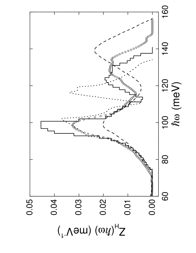
Figure 2: Hydrogen-projected density of phonon states in LiH. The experimentally-determined result is plotted as circles, the full line represents a DDM13 lattice dynamics simulation,Dyck the dashed line a SM7 lattice dynamics simulation,Verble and the dotted line the old neutron measurement.Zemlianov

where $m_{\rm H}$ is the proton mass. The result for $Z_{\rm H}(\omega)$ is plotted in Fig. 2. Equation (2), and the other formulas Colo used to work out $Z_{\rm H}(\omega)$, are formally exact only in the framework of the harmonic approximation, but they have a practical validity that is far more general, as explained by Glyde Glyde in the context of solid helium. From $Z_{\rm H}(\omega)$, making use of normal and Bose-corrected moment sum rules, Turchin we are able to derive three important quantities related to the hydrogen dynamics in this hydride, namely the H mean squared displacement $\langle{\bf u}^{2}_{\rm H}\rangle$, the H mean kinetic energy $\langle T_{\rm H}\rangle$, and the H Einstein frequency, $\Omega_{0,{\rm H}}$:

$$\langle{\bf u}^{2}_{\rm H}\rangle = \frac{3\hbar}{2m_{\rm H}}\int_{0}^{\infty}d\omega\frac{Z_{\rm H}(\omega)}{\omega}\coth\left(\frac{\hbar\omega}{2k_{B}T}\right)~{},$$

$$\langle T_{\rm H}\rangle = \frac{3\hbar}{4}\int_{0}^{\infty}d\omega Z_{\rm H}(\omega)~{}\omega\coth\left(\frac{\hbar\omega}{2k_{B}T}\right)~{},$$

$$\Omega^{2}_{0,{\rm H}} = \int_{0}^{\infty}d\omega Z_{\rm H}(\omega)~{}\omega^{2}~{}.$$ (3)

As for the first, we found: $\langle{\bf u}^{2}_{\rm H}\rangle=0.062(1)$ Ų, while for the second: $\langle T_{\rm H}\rangle=80(1)$ meV, and finally for the last: $\hbar\Omega_{0,{\rm H}}=109.2(9)$ meV.

III Variational Monte Carlo Simulation

We have studied the ground-state properties of solid LiH by means of the variational Monte Carlo (VMC) method.Reynolds VMC is a fully quantum approach which relies on the variational principle; it has been extensively used in the past in microscopic calculations of quantum crystals,Kalos mainly ⁴He and ³He. Assuming only pair-wise interactions between the different atoms in the crystal, the Hamiltonian describing LiH is:

$$H=-\frac{\hbar^{2}}{2m_{\rm H}}\sum_{i=1}^{N_{\rm H}}\mbox{\bf$\nabla$}_{i}^{2}-\frac{\hbar^{2}}{2m_{\rm Li}}\sum_{i=1}^{N_{\rm Li}}\mbox{\bf$\nabla$}_{i}^{2}+\sum_{i<j}^{N_{\rm H}}V^{({\rm H},{\rm H})}(r_{ij})+\sum_{i<j}^{N_{\rm Li}}V^{({\rm Li},{\rm Li})}(r_{ij})+\sum_{i,j}^{N_{\rm H},N_{\rm Li}}V^{({\rm H},{\rm Li})}(r_{ij})\ ,$$ (4)

where $r_{ij}$ is the distance between the atoms composing an $i,j$ pair; $m_{\rm Li}$ is the Li average atomic mass; $N_{\rm H}$ and $N_{\rm Li}$ stand for the number of H and Li atoms, respectively; and $V^{({\rm H},{\rm H})}$, $V^{({\rm Li},{\rm H})}$ and $V^{({\rm Li},{\rm Li})}$ represent the three pair-wise interaction potentials. The variational principle states that for a given trial wave-function $\Psi$, the expected value of $H$ is an upper bound to the ground-state energy $E_{0}$:

$$\frac{\left\langle\Psi|H|\Psi\right\rangle}{\left\langle\Psi|\Psi\right\rangle}=E\geq E_{0}\ .$$ (5)

The multidimensional integral required in the calculation of Eq. (5) can not be evaluated exactly by analytical summation methods like, for example, the hypernetted chain formalism.Rosati However, a stochastic interpretation of this integral is rather straightforward, and this is actually the task carried out by the VMC method, with the only cost of some statistical noise.

A key point in the method is the search for a trial wave-function with a sizeable overlap with the true ground-state wave-function $\Psi_{0}$. An extensively tested model in quantum crystals is the Nosanow-Jastrow trial wave-function.Glyde ; Kalos According to this description, the wave-function is written as a product of a Jastrow factor $F$, accounting for the correlations induced by the interatomic potentials, and a phase dependent term $\Phi$, which introduces the crystal symmetries in the problem:

$$\Psi=F\Phi\ .$$ (6)

The Jastrow factor contains two-body correlation functions between the different pairs $f^{({\rm H},{\rm H})}$, $f^{({\rm Li},{\rm Li})}$ and $f^{({\rm H},{\rm Li})}$:

$$F=\prod_{i<j}^{N_{\rm H}}f^{({\rm H},{\rm H})}(r_{ij})\prod_{i<j}^{N_{\rm Li}}f^{({\rm Li},{\rm Li})}(r_{ij})\prod_{i,j}^{N_{\rm H},N_{\rm Li}}f^{({\rm H},{\rm Li})}(r_{ij})\ ,$$ (7)

and $\Phi$ localizes each particle around the lattice equilibrium sites of the crystal phase ${\bf R}_{i}^{\alpha}$ through the functions $g^{({\rm H})}$ and $g^{({\rm Li})}$:

$$\Phi=\prod_{i}^{N_{\rm H}}g^{({\rm H})}(|{\bf r}_{i}-{\bf R}_{i}^{\rm H}|)\prod_{i}^{N_{\rm Li}}g^{({\rm Li})}(|{\bf r}_{i}-{\bf R}_{i}^{\rm Li}|)\ .$$ (8)

The VMC simulation is carried out at a molar volume $v_{0}=10.059$ cm³, which is the experimentally estimated value at zero pressure and zero temperature.Besson ; Hama The lattice constant, derived from the experimental molar volume $v_{0}$, is $a=4.0578$ Å. The calculation is worked out with a simulation cubic box containing 108 particles of each type with periodic boundary conditions. We have checked that this number of particles is large enough for practically eliminating size effects on the more relevant quantities in the present study: the H mean kinetic energy, its mean squared displacement around the lattice sites, and its Einstein frequency.

As we have seen in the introductory section, LiH and the rest of hydrides and deuterides of light alkali metals are well described as ionic crystals. This nearly perfect ionic bonding allows for a model in which ions H^- and Li⁺, both with a 1s² electronic configuration, are occupying the lattice sites of the crystal. The present simulation relies on this model, assuming rigid closed-shell ions interacting via central interatomic potentials. The overlap repulsion potential between the ions is taken from the semi-empirical Born-Mayer interaction,Born and van der Waals attractive terms are also included to deal with polarizability effects. According to this general scheme, as previously mentioned, Haque and Islam Haque proposed their pair potential $V_{\rm HI}^{(\alpha,\beta)}(r)$:

$$V_{\rm HI}^{(\alpha,\beta)}(r)=B_{\alpha\beta}\exp{\left(-A_{\alpha\beta}r\right)}-\frac{C_{\alpha\beta}}{r^{6}}\ ,$$ (9)

with $\{\alpha$, $\beta\}$ = Li, H. The set of parameters entering $V_{\rm HI}^{(\alpha,\beta)}(r)$ is reported in Tab. I. In order to evaluate the influence of the interatomic potentials in our results we have also used the model proposed by Sangster and Atwood,Sangster $V_{\rm SA}^{(\alpha,\beta)}(r)$:

$$V_{\rm SA}^{(\alpha,\beta)}(r)=B_{\alpha\beta}\exp{\left[A_{\alpha\beta}\left(E_{\alpha\beta}+F_{\alpha\beta}-r\right)\right]}-\frac{C_{\alpha\beta}}{r^{6}}-\frac{D_{\alpha\beta}}{r^{8}}\ ,$$ (10)

which incorporates a dipole-quadrupole attractive term. The parameters for LiH, which are taken from Hussain and Sangster Huss (see also Sect. I), are reported in Tab. II.

The main task in a variational approach like the present one is to seek for a good trial wave-function $\Psi$ (Eqs. (6-8)). Like in solid helium calculations,Kalos we have chosen analytical two-body $f^{(\alpha,\beta)}(r)$ (see Eq. (7)) and one-body $g^{(\alpha)}(r)$ (see Eq. (8)) correlation factors with a set of free parameters to be optimized. In particular, $f^{(\alpha,\beta)}(r)$ is of McMillan type:Mcmillan

$$f^{(\alpha,\beta)}(r)=\exp{\left[-\frac{1}{2}\left(\frac{b_{\alpha\beta}}{r}\right)^{5}\right]}\ ,$$ (11)

and the specific phase factor is a Gaussian centered on the sites of the crystal lattice:

$$g^{(\alpha)}(r)=\exp{\left(-\frac{1}{2}\,c_{\alpha}r^{2}\right)}\ .$$ (12)

In the optimization search the absolute minimum of the internal energy $\langle H\rangle_{\Psi}$ is looked for. However, the number of parameters is large enough to make this optimization rather difficult. In order to discern between local minima of similar quality we have also calculated the energy of the solid including Coulomb contributions, considering the ions as point-like particles. Under this criterion, the final parameter set is the one which simultaneously minimizes the short-range energy and the total energy including Coulomb contributions. The values obtained, which are the same for the two short-range potentials $V_{\rm HI}$ and $V_{\rm SA}$, are: $c_{\rm Li}=150$ Å^-2, $c_{\rm H}=15$ Å^-2, $b_{{\rm Li}{\rm H}}=2.0$ Å, $b_{{\rm Li}{\rm Li}}=1.5$ Å, and $b_{{\rm H}{\rm H}}=1.0$ Å. Among the three $b_{\alpha\beta}$ Jastrow parameters, the most important is the cross one ($b_{{\rm Li}{\rm H}}$), since the first neighbors of a H^- ion are Li⁺, and vice versa. It is worth noticing that the optimal values for $c_{\alpha}$ reflect the difference in the degree of localization around the sites between the two ions due to their significantly different masses, $c_{\rm H}<<c_{\rm Li}$. Including the Coulomb potential in the energy, the energies per particle are -5.07(2) eV and -5.32(2) eV for the $V_{\rm HI}$ and $V_{\rm SA}$ short-range potentials, respectively.

Information on the spatial structure of the solid can be drawn from the two-body radial distribution functions $g^{(\alpha,\beta)}(r)$. In Fig. 3, results for the three components $g^{(\alpha,\beta)}(r)$ are shown. As expected, the location of the peaks follows the inter-particle pattern imposed by the lattice: each ion is surrounded by ions of opposite sign and ions of equal sign are distributed with the same periodicity. The major mobility of H^- with respect to Li⁺ is also observed by comparing the height and the spreading around the sites of $g^{({\rm Li},{\rm Li})}(r)$, on one hand, and $g^{({\rm H},{\rm H})}(r)$ and to a lesser extend $g^{({\rm Li},{\rm H})}(r)$, on the other.

A structural quantity which can be directly compared with the present experimental data is the mean squared displacement of the H^- ions, $\langle{\bf u}^{2}_{\rm H}\rangle$:

$$\langle{\bf u}^{2}_{\rm H}\rangle=\frac{1}{N_{\rm H}}\,\left\langle\sum_{i=1}^{N_{\rm H}}\left({\bf r}_{i}-{\bf R}_{i}^{\rm H}\right)^{2}\right\rangle\ .$$ (13)

Using the trial wave-function quoted above, the VMC result is $\langle{\bf u}^{2}_{\rm H}\rangle=0.074(2)$Ų. The resulting Lindemann ratio:

$$\gamma_{\rm H}=\frac{2\sqrt{\langle{\bf u}^{2}_{\rm H}\rangle}}{a}\ ,$$ (14)

is 0.134. Additional insight on the spatial localization of H^- can be obtained by calculating the H^- density profile $u_{\rm H}(r)$, with $r$ being the distance between the ion and its site. The function $u_{\rm H}(r)$ is shown in Fig. 4; it is very well parameterized by a Gaussian with the VMC expected value $\langle{\bf u}^{2}_{\rm H}\rangle=0.074(1)$ Ų (see the solid line in the same figure).

The kinetic energy per particle of H^- is one of the partial contributions to the total energy of the solid, which is evaluated at each step of the VMC simulation. It is the expected value of the operator:

$$\langle T_{\rm H}\rangle=-\frac{\hbar^{2}}{2m_{\rm H}N_{\rm H}}\left\langle\sum_{i=1}^{N_{\rm H}}\frac{\mbox{\bf$\nabla$}_{i}^{2}\Psi}{\Psi}\right\rangle\ ,$$ (15)

with configuration points generated according to the probability distribution function $|\Psi|^{2}$. As in the estimation of $\langle{\bf u}^{2}_{\rm H}\rangle$, the H^- kinetic energy is the same for the two interatomic potentials (Eqs. 9,10) since the optimization procedure has led to the same variational wave-function. The result obtained is $\langle T_{\rm H}\rangle=84(1)$meV.

The third physical quantity evaluated in the present experiment, the Einstein frequency $\Omega_{0,{\rm H}}$, can be calculated in a VMC simulation through its proper definition:

$$\Omega_{0,{\rm H}}^{2}=\frac{1}{3m_{\rm H}N_{\rm H}}\left\langle\sum_{i=1}^{N_{\rm H}}\mbox{\bf$\nabla$}_{i}^{2}V_{\rm H}({\bf r}_{i})\right\rangle\ ,$$ (16)

where the expected value of $\mbox{\bf$\nabla$}_{i}^{2}V_{\rm H}(r)$ is calculated over the configurations generated by the probability distribution function $|\Psi|^{2}$, and $V_{\rm H}(r)$ is the potential felt by an H^- ion:

$$V_{\rm H}({\bf r}_{i})=\frac{1}{2}\sum_{j\neq i}^{N_{\rm H}}V^{({\rm H},{\rm H})}(r_{ij})+\frac{1}{2}\sum_{j=1}^{N_{\rm Li}}V^{({\rm H},{\rm Li})}(r_{ij})\ .$$ (17)

The result obtained applying Eq. (16) is $\hbar\Omega_{0,{\rm H}}=110.3(5)$ meV.

IV Discussion

The aim of this discussion section is threefold: 1) critically analyzing various dynamical quantities derived from the scientific literature with respect to the present results obtained through neutron scattering (Subsect. A); 2) comparing the outputs of the experimental and theoretical approaches presently used, namely IINS and VMC simulations (Subsect. B); 3) finally, shedding some light on the important point of the possible quantum anharmonic effects on the H^- dynamics in low-temperature LiH (Subsect. C).

IV.1 Analysis of the H-DoPS evaluations

A comparison among the various determinations (both experimental and simulated) of the hydrogen-projected density of phonon states could be finally established at this stage. In Fig. 2, four H-DoPS estimates have been plotted together in the frequency region concerning the two optical bands ($65$ meV $<\hbar\omega<160$ meV), namely the translational optical (TO) and the longitudinal optical (LO), which actually contain more than $97$% of the total $Z_{\rm H}(\omega)$ area. Dyck The present IINS experimental result is plotted as circles, the full line represents the DDM13 lattice dynamics simulation, Dyck the dashed line is the SM7 lattice dynamics simulation, Verble and the dotted line stands for the old IINS measurement. Zemlianov As a preliminary comment, one can easily observe the existence of a fair general agreement among all the four $Z_{\rm H}(\omega)$ in the TO range, at least as far as the peak position is concerned. On the contrary, the LO region looks much more uncertain, the peak centroid varying from 115 meV up to 140 meV. The reason for such a behavior is easily understandable for SM7 and DDM13 data: these lattice dynamics calculations made use of the some parameters (7 and 13, respectively) derived from a fit of the same LiD dispersion curves measured by Verble Verble (for a detailed comparative discussion on the differences between the SM7 and DDM13 H-DoPS calculations see Ref. [Dyck, ]). By a simple inspection of these experimental dispersion curves, it is clear that the LO neutron groups are really few (four values plus one infra-red measurement at the $\Gamma$ point). However the disagreement between the present IINS $Z_{\rm H}(\omega)$ and the old one is difficult to explain, so that we are inclined to think that these discrepancies are due to experimental imperfections in the data analysis of the latter (e.g. multiple scattering or multiphonon scattering subtraction). Selecting the two most recent experimental and simulated $Z_{\rm H}(\omega)$, namely the present IINS and the DDM13 estimates, we can observe an overall semi-quantitative agreement, the main discrepancies being concentrated in two regions: at low energy, in the onset of TO band ($65$ meV $<\hbar\omega<90$ meV), and in the LO band as a whole ($112$ meV $<\hbar\omega<145$ meV). As for the latter, a simple energy shift of $4.5$ meV seems sufficient to largely reconcile IINS and DDM13, while in the former case, neutron data appear somehow broader than lattice dynamical ones (IINS FWHM being about $5.1$ meV larger than DDM13 FWHM). Considering the TOSCA-II energy resolution in this region ($\Delta\hbar\omega\simeq 1.6$ meV), a simple explanation based only on experimental effects can be easily discarded. However, as pointed out by Izyumov and Chernoplekov for other hydrides, Izyumov such a broadening of the H-DoPS TO bands might be the mark of the hydrogen anharmonic dynamics in LiH, through a finite phonon life-time. In this respect, more will be said in Subsect. C.

IV.2 Comparison between IINS and VMC results

Since VMC, as we have seen in Sect. III, is a ground-state method, $Z_{\rm H}(\omega)$ can not be directly evaluated. However, through the aforementioned normal and Bose-corrected moment sum rules in Eqs. (II), it was possible to describe the main features of the H-DoPS via $\langle{\bf u}^{2}_{\rm H}\rangle$, $\langle T_{\rm H}\rangle$ and $\Omega_{0,{\rm H}}$, which are equilibrium quantities calculated by the VMC code (see also Sect. III). Before proceeding with this comparison, it is worth noticing that the VMC calculation is performed at zero temperature, whereas the measure is accomplished at $T=20.1(1)$ K. However, thermal effects are negligible since the Debye temperature of LiH is approximately $1100$ K,Islam and therefore the measured system can be certainly considered in its ground state, at least as far as the H^- ion dynamics is concerned. This assumption can be easily proved by calculating (always from the experimental $Z_{\rm H}(\omega)$) the zero-point values of the H mean squared displacement and mean kinetic energy, setting $T=0$: $\langle{\bf u}^{2}_{\rm H}\rangle(T=0)=0.062(1)$Ų and $\langle T_{\rm H}\rangle(T=0)=$80(1) meV, identical within the errors to the values estimated at $T=20.1$ K in Sect. II.

Going back to VMC, one can notice a value of the zero-point H mean squared displacement ($0.074(2)$ Ų, as in Sect. III) slightly higher than the IINS experimental measure. In addition these two figure have to be compared to the most recent neutron diffraction estimate by Vidal and Vidal-Valat:Vid $\langle{\bf u}^{2}_{\rm H}\rangle=$0.0557(6) Ų (extrapolated at $T=20$ K by the present authors from the original data in the temperature range $93$ K$-293$ K), which appears close but still discrepant from the VMC and IINS findings. However, it has to be pointed out that a previous room-temperature diffraction result by Calder et al.,Calder $\langle{\bf u}^{2}_{\rm H}\rangle=$0.068(1) Ų, seems to exhibit a similar trend if compared to the Vidal and Vidal-Valat’s figure in the same conditions: $\langle{\bf u}^{2}_{\rm H}\rangle=$0.0650(6) Ų. On the other hand, for the other two aforementioned physical quantities, the agreement between IINS ($\langle T_{\rm H}\rangle=80(1)$ meV, $\hbar\Omega_{0,{\rm H}}=109.2(9)$ meV) and VMC ($\langle T_{\rm H}\rangle=84(1)$ meV, $\hbar\Omega_{0,{\rm H}}=110.3(5)$ meV) is much more satisfactory, confirming the validity of our combined IINS-VMC method.

An interesting test on the obtained results can be accomplished in the framework of an approximate estimation known as the Self Consistent Average Phonon (SCAP) formalism.Shukla ; Paskin The SCAP approach relies on the well-known Self Consistent Phonon (SCP) method, but replacing the sums of functions of the phonon frequencies by appropriate functions of an average-phonon frequency. Results Paskin for quasi-harmonic and harmonic solids like Ne, Kr, and Xe obtained using SCAP have shown good agreement with experimental data. The application of this formalism to quantum crystals seems however more uncertain due to the relevant increase of anharmonicity. As LiH seems to be a quantum crystal, but with less anharmonicity than for example ⁴He, SCAP can somehow help in the present study. Normally SCAP is used to evaluate various physical quantities in an iterative way, employing lattice parameters and interatomic potentials only.Shukla Here, on the contrary, the method will be applied in one single step, starting from “exact” values of $\Omega_{0,{\rm H}}$. To this end, we have calculated via SCAP (at $T=0$) the H mean squared displacement and mean kinetic energy using the relations:

$$\langle{\bf u}_{\rm H}^{2}\rangle^{\rm(SCAP)} = \frac{3\hbar}{2m_{\rm H}\Omega_{0,{\rm H}}}~{},$$

$$\langle T_{\rm H}\rangle^{\rm(SCAP)} = \frac{1}{2}~{}m_{\rm H}\langle{\bf u}_{\rm H}^{2}\rangle^{\rm(SCAP)}\Omega_{0,{\rm H}}^{2}=\frac{3}{4}\hbar\Omega_{0,{\rm H}}~{}.$$ (18)

The results obtained through this approximation are: $\langle{\bf u}^{2}_{\rm H}\rangle^{\rm(SCAP-VMC)}=0.0564(3)$ Ų, $\langle{\bf u}^{2}_{\rm H}\rangle^{\rm(SCAP-IINS)}=0.0570(5)$ Ų, $\langle T_{\rm H}\rangle^{(\rm SCAP-VMC)}=82.7(4)$ meV, and $\langle T_{\rm H}\rangle^{\rm(SCAP-IINS)}=81.9(7)$ meV. By comparing these approximated values with the microscopic ones, one realizes that the H mean kinetic energy values come out very close, but the SCAP values of the mean squared displacement are significantly smaller, actually not far from the neutron diffraction result by Vidal and Vidal-Valat.Vid The physical meaning of these results is straightforward: both SCAP equations are exact at $T=0$ in presence of a purely harmonic Einstein solid (i.e. if $Z_{\rm H}(\omega)=$$\delta\left(\omega-\Omega_{0,{\rm H}}\right)$ ). But if the solid system exhibits a broader H-DoPS, then $\langle{\bf u}_{\rm H}^{2}\rangle^{\rm(SCAP)}$ comes out rather underestimated, since $\Omega_{0,{\rm H}}^{2}$ is exactly computed stressing the high-frequency part of $Z_{\rm H}(\omega)$ via the integrand factor $\omega^{2}$ (as in Eqs. (II)). In this way, one somehow corrects for this bias by expressing the zero-point mean kinetic energy as the product of $\langle{\bf u}^{2}_{\rm H}\rangle^{\rm(SCAP)}$ times $\Omega_{0,{\rm H}}^{2}$, because $\langle T_{\rm H}\rangle$ would be exactly evaluated via the integrand factor $\omega$ (see Eqs. (II)), which still stress the high-frequency part of $Z_{\rm H}(\omega)$, but less than $\Omega_{0,{\rm H}}^{2}$. Nevertheless, it is quite remarkable the good accuracy achieved by this relatively simple approach in evaluating the mean kinetic energy, probably beyond what is a priori expected for a system with a possible quantum-crystal character like LiH.

IV.3 Possible quantum anharmonic effecs in LiH

Given the relatively large value of the H Lindemann ratio in LiH ($\gamma_{H}\simeq(0.12-0.13)$ as seen above), it is natural to inquire on the low-temperature anharmonic effects in the H^- ion dynamics. In this respect our tools are well suited, since VMC is a microscopic quantum simulation, assuming neither the harmonic approximation like the usual lattice dynamic calculations, nor the semi-classical treatment of the particle motion like the molecular dynamics approach.semicl The method applied to test the existence of possible quantum anharmonic effects in H dynamics (at $T=0$) was simply devised running the same VMC code in a “harmonic way”, i.e., replacing for every atomic pair $i,j$ the exact pair potential value $V^{(\alpha,\beta)}(r_{ij})$ by:Wallace

$$V^{(\alpha,\beta)}(r_{ij})\simeq V^{(\alpha,\beta)}(r_{0,ij})+\frac{1}{2}\left({\bf u}_{i}-{\bf u}_{j}\right)^{\rm T}\left(\frac{\partial^{2}V^{(\alpha,\beta)}(r_{ij})}{\partial{\bf r}_{ij}\partial{\bf r}_{ij}}\right)_{r_{ij}=r_{0,ij}}\left({\bf u}_{i}-{\bf u}_{j}\right)~{},$$ (19)

where ${\bf r}_{i}$ and ${\bf u}_{i}$ are the instantaneous position of an $i$ atom and its displacement from the equilibrium position, respectively, while ${\bf r}_{ij}$ stands for the vector ${\bf r}_{i}-{\bf r}_{j}$, and $r_{0,ij}$ is the equilibrium separation of an atomic pair $i,j$. It is worth noting that both the static potential energy $V^{(\alpha,\beta)}(r_{0,ij})$ and the Hessian components are all calculated only once per each atomic pair $i,j$, since they depend only on the equilibrium distance $r_{0,ij}$. However the “harmonic” results from VMC did not show any significant difference (within their uncertainties) from the “exact” ones (see above in Subsect. B), proving that, at least in the framework of the semi-empirical pair potentials employed, quantum anharmonic effects are totally negligible in the evaluation of $\langle{\bf u}^{2}_{\rm H}\rangle$ and $\langle T_{\rm H}\rangle$, even at $T=0$.

V Conclusions and perspectives

Dynamical properties of solid LiH at low temperature have been studied using incoherent inelastic neutron scattering with higher accuracy than in previous measurements. The analysis of the scattering data has allowed for the extraction of a reliable hydrogen-projected density of phonon states. From this physical quantity it was possible to estimate three relevant quantities intimately related to the microscopic dynamics of H in the solid: its mean squared displacement, mean kinetic energy, and Einstein frequency. Apart from the intrinsic interest in an accurate quantitative determination of these magnitudes, we have tried to shed some light on two fundamental questions on the physical nature of LiH, i.e. its quantum character and the degree of anharmonicity in the H dynamics. To this end, and also to make a direct comparison with theory, we have carried out a quantum microscopic calculation of the same three quantities quoted above using VMC.

The consideration of solid LiH as a quantum solid seems already justified by its Lindemann ratio which is smaller than the two paradigms, ⁴He and ³He, but still appreciably larger than the common values in classical solids. From a theoretical viewpoint, it supposes the unavoidable introduction of at least two-body correlations to account correctly for its ground-state properties. We have verified using VMC that this feature also holds in solid LiH.

The degree of anharmonicity in H dynamics has been established by comparing the full VMC calculation with another one in which the real interatomic potentials have been substituted by harmonic approximations (Eq. (19)). As commented in the previous Section, both VMC simulations generate identical results and then possible anharmonic effects in H are not observed. This situation is different from the one observed in solid ⁴He where quantum character and anharmonicity appear together. Apart from the appreciable difference between both systems looking at their respective Lindemann ratios, a relevant feature that can help to understand the absence of anharmonicity of H in LiH is the significant difference between the interatomic potentials at short distances in both systems. Helium atoms interact with a hard core of Lennard-Jones type whereas the short-range interaction between the components of the mixture LiH is much softer (exponential type) according to the Born-Mayer model.

The agreement achieved in the present work between the neutron scattering data and the VMC calculation is remarkably good and probably better than what could be initially expected from the use of semi-empirical interactions. The VMC predictions for the H kinetic energy and Einstein frequency coincide within error bars with the experimental measures. On the contrary, the H mean square displacement is about $15$% larger. This points to probable inaccuracies of the model potentials, in particular, to core sizes smaller than the real ones. In this respect, it has also to be said that these semi-empirical potentials have been proposed and evaluated in order to reproduce various LiH properties (e.g. lattice constant, bulk modulus, reststrahl frequency, etc.)Huss ; Haque ; Sangster in the framework of the standard (i.e. harmonic) lattice dynamics. Thus, the ab initio calculation of more realistic pair interactions could help enormously to improve a microscopic description of LiH and justify for the future the use of techniques beyond VMC, like the diffusion Monte Carlo or path integral Monte Carlo methods.

$\alpha$	$\beta$	$A_{\alpha\beta}$(Å-1)	$B_{\alpha\beta}$(eV)	$C_{\alpha\beta}$(eVÅ6)
Li	Li	7.3314	1153.80	0.0
Li	H	3.1000	187.29	0.0
H	H	5.5411	915.50	4.986

Table 1: Parameters of the $V_{\rm HI}^{(\alpha,\beta)}(r)$ potential by Haque and Islam.Haque

$\alpha$	$\beta$	$A_{\alpha\beta}$(Å-1)	$B_{\alpha\beta}$(eV)	$E_{\alpha\beta}$(Å)	$F_{\alpha\beta}$(Å)	$C_{\alpha\beta}$(eVÅ6)	$D_{\alpha\beta}$(eVÅ8)
Li	Li	38.48731	17.8000	0.2226	0.2226	0.0549073	0.0216285
Li	H	3.784068	0.17675	0.2226	1.9000	0.9568660	2.0013052
H	H	2.608380	0.01422	1.9000	1.9000	48.872096	185.18284

Table 2: Parameters of the $V_{\rm SA}^{(\alpha,\beta)}(r)$ potential proposed by Sangster and Atwood,Sangster estimated by Hussain and Sangster.Huss

Figure 1: Neutron scattering spectra from LiH at $T=20.1(1)$ K: (a) TOSCA-II experimental data (circles) together with the estimate of the multiple scattering contribution (line); (b) experimental scattering law (circles) and its multiphonon component (line).

Figure 3: Two-body radial distribution functions in LiH: $g^{({\rm H},{\rm Li})}(r)$, solid line; $g^{({\rm H},{\rm H})}(r)$, dashed line; $g^{({\rm Li},{\rm Li})}(r)$, dotted line.

Figure 4: Variational Monte Carlo result for the H^- density profile, $u_{\rm H}(r)$, in LiH. The solid line corresponds to a Gaussian with a mean squared displacement equal to the variational Monte Carlo value $\langle{\bf u}^{2}_{\rm H}\rangle=0.074$ Ų.

References

- (1) W. M. Mueller, J. P. Blackledge, and G. G. Libowitz, Metal Hydrides (Academic Press, New York, 1968).
- (2) E. Zintl and A. Harder, Z. Phys. Chem. B 14, 265 (1931).
- (3) R. S. Calder, W. Cochran, D. Griffiths, and R. D. Lowde, J. Phys. Chem. Solids 23, 621 (1962).
- (4) C. O. Rodriguez and K. Kunc, J. Phys.; Condensed Matter 1, 1601 (1989).
- (5) An extensive review is in A. K. M. A. Islam, Phys. Stat. Sol. B 180, 9 (1993).
- (6) J. Van Kranendonk, Solid Hydrogen (Plenum Press, New York, 1983).
- (7) H. R. Glyde, Excitations in Liquid and Solid Helium (Oxford U. P., Oxford, 1994).
- (8) F. A. Lindemann, Phys. Z. 11, 609 (1911).
- (9) J. P. Vidal and G. Vidal-Valat, Acta Cryst. B 42, 131 (1986).
- (10) J. M. Besson, G. Weill, G. Hamel, R. J. Nelmes, J. S. Loveday, and S. Hull, Phys. Rev. B 45, 2613 (1992).
- (11) A. C. Ho, R. C. Hanson, and A. Chizmeshya, Phys. Rev. B 55, 14818 (1997).
- (12) S. Lebèsgue, M. Alouani, B. Arnaud, and W. E. Pickett, Europhys. Lett. 63, 562 (2003).
- (13) J. L. Verble, J. L. Warren, and J. L. Yarnell, Phys. Rev. 168, 980 (1968).
- (14) W. Dyck and H. Jex, J. Phys. C.: Solid State Phys. 14, 4193 (1981).
- (15) Yu. A. Izyumov and N. A. Chernoplekov, Neutron Spectroscopy (Consultants Bureau, New York, 1994).
- (16) M. G. Zemlianov, E. G. Brovman, N. A. Chernoplekov, and Yu. L. Shitikov, in Inelastic Scattering of Neutrons, vol. II, pg. 431 (IAEA, Vienna, 1965).
- (17) A. R. Q. Hussain and M. J. Sangster J. Phys. C.: Solid State Phys. 19, 3535 (1986).
- (18) E. Haque and A. K. M. A. Islam, Phys. Stat. Sol. B 158, 457 (1990).
- (19) G. Roma, C. M. Bertoni, and S. Baroni, Solid State Communications 98 203 (1996).
- (20) B. Yates, G. H. Wostenholm, and J. L. Bingham, J. Phys. C: Solid State Phys. 7, 1769 (1974).
- (21) J. L. Anderson J. Nasise, K. Philipson, and F. E. Pretzel, J. Phys. Chem. Solids 31, 613 (1970).
- (22) D. C. Wallace, Thermodynamics of Crystals (J. Wiley, New York, 1972).
- (23) D. Colognesi, M. Celli, F. Cilloco, R. J. Newport, S. F. Parker, V. Rossi-Albertini, F. Sacchetti, J. Tomkinson, and M. Zoppi, Appl. Phys. A 74 [Suppl. 1], 64 (2002).
- (24) S. F. Parker, private communication to the authors (2004).
- (25) S. W. Lovesey, Theory of Neutron Scattering from Condensed Matter, vol. I (Oxford University Press, Oxford, 1987).
- (26) A. K. Agrawal, Phys. Rev. A 4, 1560 (1971).
- (27) D. Colognesi, C. Andreani, and E. Degiorgi, Phonon Density of States from a Crystal-analyzer Inverse-geometry Spectrometer: A study on Ordered Solid Hydrogen Sulfide and Hydrogen Chloride in press on Journal of Neutron Research (2003).
- (28) A. I. Kolesnikov and J.-C. Li, Physica B 234-236, 34 (1997); J. Dawidowski, F. J. Bermejo, and J. R. Granada, Phys. Rev. B 58, 706 (1998).
- (29) V. F. Turchin, Slow Neutrons (Israel Program for Scientific Translations, Jerusalem, 1965).
- (30) J. Hama and N. Kawakami, Phys. Lett. A 126, 348 (1988).
- (31) M. Born and K. Huang, Dynamical Theory of Crystal Lattices (Oxford Press, Oxford, 1954).
- (32) B. L. Hammond, W. A. Lester Jr., and P. J. Reynolds, Monte Carlo Methods in Ab Initio Quantum Chemistry (World Scientific, Singapore, 1994).
- (33) D. M. Ceperley and M. H. Kalos, in Monte Carlo Methods in Statistical Physics, edited by K. Binder (Springer, Berlin, 1979).
- (34) S. Rosati and M. Viviani, in First International Course on Condensed Matter, edited by D. Prosperi et al. (World Scientific, Singapore, 1988)
- (35) M. J. L. Sangster and R. M. Atwood, J. Phys. C: Solid State Phys. 11, 1541 (1978).
- (36) W. L. McMillan, Phys. Rev. 138, 442 (1965).
- (37) K. Shukla, A. Paskin, D. O. Welch, and G. J. Dienes, Phys. Rev. B 24, 724 (1981).
- (38) A. Paskin, A. M. Llois de Kreiner, K. Shukla, D. O. Welch, and G. J. Dienes, Phys. Rev. B 25, 1297 (1982).
- (39) M. T. Dove, Introduction to Lattice Dynamics (Cambridge University Press, Cambridge, 1993).