Anomalous scaling of conductivity in integrable fermion systems

Abstract

We analyze the high-temperature conductivity in one-dimensional integrable models of interacting fermions: the $t$-$V$ model (anisotropic Heisenberg spin chain) and the Hubbard model, at half-filling in the regime corresponding to insulating ground state. A microcanonical Lanczos method study for finite size systems reveals anomalously large finite-size effects at low frequencies while a frequency-moment analysis indicates a finite d.c. conductivity. This phenomenon also appears in a prototype integrable quantum system of impenetrable particles, representing a strong-coupling limit of both models. In the thermodynamic limit, the two results could converge to a finite d.c. conductivity rather than an ideal conductor or insulator scenario.

I Introduction

Transport of strongly interacting fermions in one-dimensional (1D) systems have been so far the subject of numerous theoretical as well as some experimental studies zprev . While the ground-state and low-temperature properties, following the Luttinger-liquid universality, are well understood, the transport properties still lack some fundamental understanding regarding the role of fermion correlations. It has become evident in recent years, that with respect to transport (in contrast to static quantities) integrable many-fermion models behave very differently from nonintegrable ones cast ; zprev . Some basic 1D fermion models are integrable, as the $t$-$V$ model (equivalent to the anisotropic Heisenberg spin model) and the Hubbard model, and reveal in the metallic regime dissipationless transport at finite temperature $T>0$, well founded due to the relation to conserved quantities zot1 ; zot2 ; fabr . The transport in the ’insulating’ regime of integrable models, however, has been controvertial and is the issue of this paper.

Let us concentrate on the dynamical conductivity in 1D system

$$\sigma(\omega) = 2\pi D\delta(\omega)+\sigma_{reg}(\omega),$$

$$\sigma_{reg}(\omega>0) = \frac{1-e^{-\beta\omega}}{\omega L}{\mathrm{R}e}\int_{0}^{\infty}dte^{i\omega t}\langle j(t)j(0)\rangle\leavevmode\nobreak\ ,$$ (1)

where $j$ is the (total) particle current operator, $\beta=1/T$ and $L$ is the number of sites in the chain (we set everywhere $k_{B}=\hbar=e_{0}=1$ as well as lattice spacing $a_{0}=1$). At finite $T$ the charge stiffness (referred to also as Drude weight) $D(T)$ measures the dissipationless component in the response, while $\sigma_{reg}(\omega)$ is the ’regular’ part. The requirement that the ground state is insulating kohn is $D_{0}=D(T=0)=0$. In the insulating regime there are still several alternative scenarios for the behavior at finite temperatures. The system can at $T>0$ behave as: a) an ’ideal conductor’ with $D(T)>0$, b) a ’normal resistor’ with $D(T)=0$ but $\sigma_{0}=\sigma(\omega\to 0)>0$, and c) an ’ideal insulator’ with $D(T)=0$ and $\sigma_{0}=0$.

A well-known $T=0$ insulator is the $t$-$V$ model at half filling and $V/t>2$. The model is equivalent in this regime to an easy-axis anisotropic XXZ Heisenberg model with $\Delta>1$. It has been shown by one of the present authors zoto that $D(T>0)$ is finite for $V/t<2$ but decreasing towards $D(T>0)=0$ at $V/t=2$. This gives a strong indication that $D(T)=0$ in the whole regime $V/t>2$, although there are also alternative interpretations pscc ; bren . The present authors speculated in this case on a possible realisation of an ’ideal insulator’ zot1 where also $\sigma_{0}(T>0)=0$. The argument is based on the observation that at least in the $V/t\to\infty$ limit the soliton-antisoliton mapping can be applied, where the eigenstates cannot carry any current. However, the issue proved to be more involved. Note that the transport of gapped spin systems described by the quantum nonlinear sigma model, when treated by a semiclassical approach sach (mapping to a model of classical impenetrable particles) indicates a ’normal conductor’ with a finite diffusion constant and $\sigma_{0}(T>0)>0$. On the other hand, a Bethe ansatz approach fuj concludes to a finite Drude weight $D(T>0)>0$ and thus ballistic transport. It should be reminded that the $V/t=2$ case, corresponding to the most studied isotropic Heisenberg model, is marginal situation, with the long-standing open question whether the diffusion constant (studied mostly at $T\to\infty$) in this model is finite carb ; fabr . Another prominent $T=0$ insulator is the Hubbard model at half filling. Here even the question of $D(T>0)$ is controvertial. On the basis of Bethe ansatz results fuji and Quantum Monte Carlo simulations kirc it is claimed that $D(T>0)>0$, i.e. an ’ideal conductor’ situation. More recent analytical considerations pere seem to favor $D(T)=0$.

The aim of this paper is to present numerical evidence that the dynamical conductivity $\sigma(\omega)$ in the insulating regime of several integrable 1D models is indeed very anomalous. We consider in this context three 1D models: the $t$-$V$ model, the Hubbard model and a related model of impenetrable particles. First, finite-size scaling of results for all mentioned models indicates that indeed $D(T>0)=0$ (whereby the evidence is somewhat less conclusive for the Hubbard model). Moreover, we show that on the one hand small-system results reveal large pseudogap features in $\sigma(\omega\sim 0)$ and large finite size effects extending to high frequencies; on the other hand, after the finite-size scaling in the thermodynamic limit is performed, the results could be consistent with a ’normal’ and featureless $\sigma(\omega)$ found by a frequency-moment analysis. In this respect the behavior is very different from the one in nonintegrable quantum many-body models where even in small-size systems a ’normal’ diffusive behavior is very evident zot1 ; zot .

The paper is organized as follows. In Sec. II we present two alternative numerical methods used to analyse the dynamical conductivity $\sigma(\omega)$: the microcanonical Lanczos method and the method of frequency moments. In Sec. III results for three different 1D models in the insulating regime are presented and discussed: the $t$-$V$ model at half-filling, the Hubbard model at half-filling and the model of impenetrable particles.

II Numerical methods

Microscopic models considered in this paper are 1D tight-binding models with the hopping only among nearest neighbors. We investigate within these models the dynamical charge conductivity $\sigma(\omega)$ (in the case of impenetrable particles the related spin conductivity $\sigma_{s}(\omega)$) at $T\to\infty$ with an emphasis on the low $\omega\to 0$ behavior. The first approach we apply is the full exact diagonalization (ED) of the Hamiltonian on a lattice with $L$ sites and periodic boundary conditions (p.b.c.) taking into account the number of fermions $N$ and the wavevector $q$ as good quantum numbers. E.g., this allows for an exact solution of $\sigma(\omega)$ up to $L=20$ for the $t$-$V$ model. Larger systems can be studied using the Lanczos method of ED.

Particularly appropriate at large enough $T$ is the microcanonical Lanczos method (MCLM) long . The MCLM uses the idea that dynamical autocorrelations (in a large enough system) can be evaluated with respect to a single wavefunction $|\Psi\rangle$ provided that the energy deviation

$$\delta\epsilon=(\langle\Psi|(H-\lambda)^{2}|\Psi\rangle)^{1/2}$$ (2)

is small enough. Clearly, $\lambda$ determines here the temperature $T$ for which $|\Psi\rangle$ is a relevant representative. Such $|\Psi\rangle$ can be generated via a first Lanczos procedure using instead of $H$ a modified projection operator $P=(H-\lambda)^{2}$, performing $M_{1}$ Lanczos steps to get the ground state of $P$. The dynamical correlations are then calculated using the standard Lanczos procedure for dynamical autocorrelation functions, where the modified $|\tilde{\Psi}\rangle=j|\Psi\rangle$ is the starting wavefunction for the second Lanczos iteration with $M_{2}$ steps generating the continued fraction representation of $\sigma(\omega)$. The main advantage of the MCLM is that it can reach systems equivalent in size to the usual ground-state calculations using the Lanczos method. For details we refer to Ref.[17]; e.g., the largest available size for the $t$-$V$ model is thus $L=28$.

Besides the $\sigma(\omega)$ spectra it is instructive to also show the normalized integrated intensity $I(\omega)$. In tight-binding models with n.n. hopping the (optical) sum rule for $\sigma(\omega)$ is given by $\langle-T\rangle/2L$ where $T$ is the kinetic term in the Hamiltonian. Hence $I(\omega)$ can be expressed as

$$I(\omega)=D^{*}+\frac{2L}{\langle-T\rangle}\int_{0^{+}}^{\omega}d\omega^{\prime}\sigma(\omega^{\prime}),$$ (3)

which is monotonously increasing function with the limiting value $I(\omega\to\infty)=1$ and well defined even for small systems. Here, $D^{*}=2LD/\langle-T\rangle$. It should be noted that in a full ED calculation the Drude part $D$ appears strictly at $\omega=0$, Eq. (1), while in the MCLM it spreads into a window $\delta\epsilon\ll t$ governed by the number of Lanczos steps $M_{1}$. Still, choosing large enough $M_{1}\sim 1000$, $\delta\epsilon$ becomes very small, hence we get well resolvable Drude contribution. Typically we use in the calculations presented here $M_{1}=1000$, $M_{2}=5000$. In order to get smooth spectra especially for small system sizes, we additionally performed an averaging over $N_{\lambda}$ different $\lambda$ with respect to the normal Gaussian distribution. Typically, we used $N_{\lambda}\sim 20$ for smallest $L$ and $N_{\lambda}\sim 1$ for largest $L$ presented in figures below.

As will be evident from results furtheron $\sigma(\omega)$ exhibits huge finite-size effects. The latter are clearly a consequence of the integrability since nonintegrable models do not exhibit such features. In order to avoid such finite-size phenomena we also perform an alternative analysis using the method of frequency moments (FM). It is well known that at $T=\infty$ one can calculate for $\sigma(\omega)$ exact frequency moments $m_{2k}=\pi\mu_{2k}/T$ as

$$\mu_{2k}={\rm Tr}([H,[H,\cdots,[H,j]]\cdots]j)/{\rm Tr}(1).$$ (4)

Moments correspond here to an infinite system $L\to\infty$ and could be evaluated at fixed fermion concentration $n=N/L$ using the linked cluster expansion and the diagrammatic representation ohat ; mori . Only clusters containing up to $k+1$ particles can contribute to $\mu_{2k}$ in an infinite system for models with n.n. connections only. However, an analytic calculation of moments for larger $k$ becomes very tedious. Hence we use the fact that exact moments for an infinite system can be obtained also via the ED results for small-system (with p.b.c.) sur provided that the system size $L$ is large enough. I.e.,

$$\mu_{2k}=\frac{1}{\Omega}\sum_{N=0}^{L}\sum_{m,l}f^{N}(\epsilon_{Nm}-\epsilon_{Nl})^{2k}|\langle\Psi_{Nm}|j|\Psi_{Nl}\rangle|^{2},$$ (5)

where $|\Psi_{Nm}\rangle$ refer to eigenstates for $N$ fermions. In Eq. (5) $\Omega=\sum_{N}N_{st}(N)f^{N}$ and fugacity $f={\rm exp}(\mu/T)$ can be related to the density

$$n=\frac{1}{\Omega L}\sum_{N}NN_{st}(N)f^{N},$$ (6)

where $N_{st}$ is the number of states for given $N$. Let us illustrate the feasibility of FM method for the 1D $t$-$V$ model. Performing full ED for all fillings $0<N<L$ on a ring we get exactly FM up to $k=L/2-1$ whereby even higher $k>L/2-1$ moments are quite accurate. Using full ED for $L=20$ we thus reach for the $t$-$V$ model exactly up to $\mu_{18}$.

Next step is to reconstruct spectra $\sigma(\omega)$ from $\mu_{2k}$ with $k=0,K$. There are various strategies how to get the spectra most representative for $K\to\infty$, expecting a smooth function $\sigma(\omega)$. We follow here the procedure proposed by Nickel nick . First, a nonlinear transformation $\omega=z+\zeta^{2}/z$ is performed where $\zeta$ is chosen as the largest eigenvalue in a truncated continued fraction representation of $\sigma(\omega)$. For $\sigma(\omega)$ then a Padé approximant $[K_{1}/K_{2}]$ is found in terms of functions of the novel variable $z$.

It should, however, be noted that FM are less sensitive to the low-$\omega$ regime, so a possible price to pay is an uncertainty in the low frequency results. In this respect MCLM and FM results really yield an alternative view of low-$\omega$ dynamics.

III Results

III.1 $t$-$V$ model

Let us first analyse the 1D $t$-$V$ model for interacting spinless fermions,

$$H=-t\sum_{i}(c^{\dagger}_{i+1}c_{i}+\mathrm{h.c.})+V\sum_{i}n_{i}n_{i+1},$$ (7)

with the repulsion $V$ between fermions on n.n. sites and the corresponding current operator

$$j=-t\sum_{i}(ic^{\dagger}_{i+1}c_{i}+\mathrm{h.c.}).$$ (8)

At half-filling, i.e., at the fermion density $n=1/2$, the ground state is metallic for $V/t<2$ and insulating for $V/t>2$. Note that by introducing a fictitious magnetic flux via the substitution $t\to te^{i\phi}$ the model turns into the anisotropic XXZ Heisenberg model for $\phi=\pi/L$ and even number of fermions.

In the following we present only results in the limit $T\to\infty$. From Eq. (1) it follows that $\sigma$ scales in this limit as $\beta$, hence we present in Fig. 1a $\sigma(\omega)/\beta$, calculated for even number of fermions for $V/t=4$ and various sizes $L=16-28$. Results for $D/\beta$ are plotted in the inset of Fig. 1b and reveal an exponential decrease with $L$, which is at the same time a challenging test for the feasibility and the sensitivity of the MCLM at larger sizes $L$.

From results in Figs. 1a,b several observations follow: a) the dissipationless component $D$ becomes negligible at large $L$ and the extrapolated value for $L=\infty$ is consistent with $D=0$  zoto , b) there is a pseudogap at low $\omega$ followed by a pronounced peak at $\omega=\omega_{p}$ and damped oscillatory features at $\omega>\omega_{p}$, almost up to the bandwidth $\sim 4t$, c) the peak and accompanied oscillations move downward with the system size approximately as $\omega_{p}\propto 1/L$, d) the pseudogap in $\sigma(\omega\to 0)$ is compensated by the peak intensity as evident from the integrated $I(\omega)$ which is essentially independent of $L$ for $\omega>\omega_{p}$, e) $I(\omega<t)$ could approach $I(\omega)\sim\sigma_{0}\omega$ for large $L$, indicative of a ’normal’ d.c. conductivity $\sigma_{0}$ in the thermodynamic limit.

Figure 1: a) Conductivity $\sigma(\omega)/\beta$ and b) integrated normalized $I(\omega)$ at $T\to\infty$ within the 1D $t$-$V$ model with $V/t=4$, obtained using the ED and the MCLM for systems with length $L$, and the frequency moment expansion. The inset shows $\mathrm{ln}(D/\beta)$ vs. $L$, where the line is guide to the eye.

When applying the FM method to the $t$-$V$ model we get

$$\Omega=(1-n)^{-L},\qquad f=n/(1-n).$$ (9)

Using full ED for $L=20$ we reach exactly up to $\mu_{18}$. In Figs. 1a.b we diplay results for $\sigma(\omega)$ obtained via the FM using $K=9$ and the corresponding [4/5] Padé approximant. The FM method proves to be very stable in particular with respect to the most interesting and sensitive value $\sigma_{0}$. Namely the latter varies only slightly between, e.g., [3/3] and [4/5] Padé approximant. Results confirm the overall agreement of MCLM and FM-method spectra apart from evident finite-size phenomena at $\omega<\omega_{p}$. It should be, however, mentioned that there are still some nonessential differences between $I(\omega)$ results even at higher $\omega>\omega_{p}$ since the MCLM results are for fixed fermion number $N=L/2$ whereas the FM corresponds to a grandcanonical averaging over all $N$ so that even lowest moments differ slightly. The general conclusion of the FM approach is that it does not show any sign of pseudogap features and thus favors quite featureless $\sigma(\omega)$ with finite $\sigma_{0}$. Essentially the same results are reproduced for $\sigma(\omega)$ analysing FM using the maximum-entropy method mead .

III.2 Hubbard model

Next let us consider the 1D Hubbard model

$$H = -t\sum_{i,s}(e^{i\phi}c_{i+1,s}^{\dagger}c_{is}+\mathrm{h.c.})+U\sum_{i}n_{i\uparrow}n_{i\downarrow},$$ (10)

$$j=-t\sum_{i,s}(ie^{i\phi}c_{i+1,s}^{\dagger}c_{is}+\mathrm{h.c.}),$$

where we take into account a possible fictitious flux $\phi$. We study the model at half filling $n=N/L=1$ where the ground state is insulating, i.e. $D_{0}=0$, for all $U>0$. In the limit $L\to\infty$ the behavior should not depend on $\phi$. Nevertheless in small systems low-$\omega$ features, in particular $D(\phi)$, depend on $\phi$. We present here calculations within the Hubbard model using the ED and the MCLM at $\phi=\pi/(2L)$ since in this case $D(\phi,T)$ is at maximum. Relative to the $t$-$V$ model, smaller sizes are reachable for the Hubbard model at $n=1$, i.e., we investigate $L=10$ performing full ED, while with the MCLM systems up to $L=16$ can be studied.

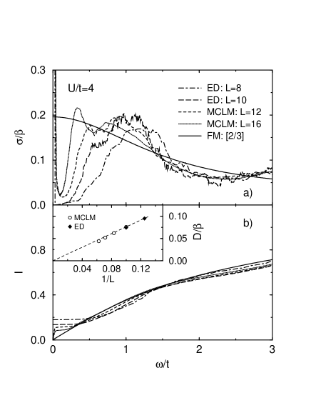
Figure 2: a) $\sigma(\omega)/\beta$ and b) $I(\omega)$ within the 1D Hubbard model with $U/t=4$, obtained via the ED, the MCLM (finite $L$) and the FM method. The inset shows $D/\beta$ scaled vs. $1/L$, whereby the line is guide to the eye.

Results for the intermediate case $U/t=4$ and again $T\to\infty$ are shown in Figs. 2a,b. We note that several features are similar to results for the $t$-$V$ model: a) $D$ decreases with $L$, b) a pseudogap appears for $\omega<\omega_{p}$, c) large finite size effects extend up to frequencies of the order of the bandwidth, d) the pseudogap scale appears to close with the increasing system size.

However, the dependence of $D(L)$ is not exponential, but the scaling appears to follow $D\propto 1/L$ (see the inset of Fig. 2b). Although with less certainty than within the $t$-$V$ model we could again support the limiting value $D(T)=0$. Also, $I(\omega)$ tends with increasing $L$ to $I\sim\sigma_{0}\omega$ for $\omega<t$, here approaching from higher values in contrast to Fig. 1b. In spite of differences to the $t$-$V$ model, results scaled to the thermodynamic limit could be consistent with a smooth $\sigma(\omega)$ and a finite $\sigma_{0}$.

We also perform the FM analysis, using exact ED results for systems with up to $L=10$ and $0<N<2L$. Here, we use

$$\Omega=(1+f)^{2L},\qquad f=n/(2-n).$$ (11)

The analysis is accurate up to $\mu_{10}$ and corresponding [3/2] Padé approximants. This is barely enough to reproduce gross features of limiting $\sigma(\omega)$, nevertheless results are in agreement with previous conclusions for the $t$-$V$ model.

III.3 Impenetrable particles

The above results indicate that integrable models in the ’insulating’ regime share similar features in the dynamical conductivity $\sigma(\omega)$. It has already been proposed zot1 that it is helpful to consider the large interaction limit, i.e., $V\gg t$ and $U\gg t$, where the dynamics of both models is simplified but remains highly nontrivial. For a half-filled band in this limit we are dealing with an excitation spectrum composed of split subspaces with a fixed number $N_{s}$ of oppositely charged “soliton-antisoliton” ($s\bar{s}$) pairs. In such a limit, the solitons/antisolitons - doubly occupied/empty sites in the Hubbard model, occupied/empty n.n. sites in the $t$-$V$ model - behave as impenetrable quantum particles, since their crossing would require virtual processes with $\Delta E=U,V$.

The simplest prototype model which incorporates the same physics - that of a system with two species of impenetrable particles - is the 1D $t$-model,

$$H=-t\sum_{is}(\tilde{c}^{\dagger}_{i+1,s}\tilde{c}_{is}+\mathrm{h.c.}),$$ (12)

where projected fermion operators take into account that the double occupation of sites is forbidden; the two species of particles are represented by the up/down spin fermions. Thus we consider within the $t$-model the spin current

$$j_{s}=t\sum_{is}(is\tilde{c}^{\dagger}_{i+1,s}\tilde{c}_{is}+\mathrm{h.c.}),$$ (13)

and the corresponding spin diffusivity $\sigma_{s}(\omega)$.

The only relevant parameter within the $t$-model is the electron density $n=n_{\uparrow}+n_{\downarrow}$, where $0<n<1$ and of interest is the paramagnetic case $n_{\uparrow}=n_{\downarrow}$. The model (12) is also exactly solvable. Moreover, the electron current $j$ commutes with $H$, while the spin current $j_{s}$ does not. It is plausible that in an unpolarized ring, $N_{\uparrow}=N_{\downarrow}$, exact eigenstates do not carry any spin current, i.e., $\langle\Psi_{n}|j_{s}|\Psi_{n}\rangle=0$, and hence $D(T)\equiv 0$. This becomes clear by introducing the fictitious flux by $t\to te^{i\phi}$. Particles cannot cross, so all eigenergies $\epsilon_{n}$ are independent of $\phi$. Since $D(T)$ can be related cast to $\partial^{2}\epsilon_{n}/\partial\phi^{2}$ this leads to $D(T)\equiv 0$. Still, this does not preclude $\sigma_{s}(\omega>0)>0$, since $\langle\Psi_{n}|j_{s}|\Psi_{m}\rangle\neq 0$ in general.

We study $\sigma_{s}(\omega)$ within the $t$-model again using the same methods. With the full ED we reach $L=12$ while with the MCLM up to $L=20$ sites. For the presentation we choose the quarter-filled case, $n=1/2$, where most systems are available, $L=8,12,16,20$. Results are shown in Figs. 3a,b. As expected, finite-size features are very similar to those in Figs. 1,2, apart from $D\equiv 0$. The pseudogap is pronounced even more clearly, with the peak frequency $\omega_{p}\propto 1/L$. Particularly powerful for this model is the FM method. Namely, from the full ED results we can evaluate exactly moments up to $\mu_{20}$. Since there is a single characteristic scale $t$, the structure of $\sigma_{s}(\omega)$ is simpler and better reproducible via the FM method. Results corresponding to [5/5] Padé approximant are presented in Figs. 3a,b and again indicate on a ’normal’ diffusivity in the thermodynamic limit.

Figure 3: a) spin diffusivity $\sigma_{s}(\omega)/\beta$ and b) the integrated $I(\omega)$ within the 1D $t$-model at $n=1/2$, obtained via the ED, the MCLM and the FM method.

IV Conclusions

Let us summarize and comment obtained results. We have shown that all considered 1D integrable models of interacting fermions share several common features:

a) The charge stiffness is either $D\equiv 0$ ($t$-model) or appears to scale to zero, whereby the evidence is stronger for the $t$-$V$ model. Whereas the vanishing $D$ is easy to understand for impenetrable particles, it is a highly nontrivial statement for the other two models pscc ; bren ; fuji ; kirc ; pere . The observations can be rationalized in a way that the $t$-$V$ and Hubbard model at half-filling in the thermodynamic limit $L\to\infty$ remain to behave as in the limit $V,U\to\infty$ where solitons and antisolitons cannot cross.

b) The pseudogap is pronounced for finite-size systems whereby the finite-size peak scales as $\omega_{p}\propto 1/L$.

c) The extrapolation to the thermodynamic limit could be compatible with a rather featureless and regular $\sigma(\omega\sim 0)$ and thus finite $\sigma_{0}$. With respect to the last two points the ED (including MCLM) and FM methods are complementary. Whereas the FM method (valid for an $L\to\infty$ system) cannot detect finite-size effects and appears to converge to a featureless $\sigma(\omega)$, the ED methods are evidently sensitive to the effect of p.b.c. at finite $L$.

A fundamental question raised by these observations is, whether the large finite size effects observed at low frequencies are reflected to the dynamics of bulk systems and in particular, which features of the conductivity (e.g. $q$,$\omega$ -dependence) might be singular.

We restricted our results to $T\rightarrow\infty$. The latter is clearly most convenient for the FM method. Nevertheless, from the MCLM results considered at finite but high $T$ there appears no evidence for any qualitative change on behavior. We also presented results for a single parameter for the $t$-$V$ and Hubbard model, and one filling for the $t$ model, respectively. One cannot expect any essential difference for other values within the ’insulating’ regime, although numerical evidence becomes poorer, e.g., on approaching $V\to 2\leavevmode\nobreak\ t$ within the $t$-$V$ model. Clearly, the most challenging case is $V=2\leavevmode\nobreak\ t$, corresponding to the isotropic Heisenberg model. Our results reveal an increase of $\sigma_{0}$ on approaching $V=2\leavevmode\nobreak\ t$. Still we are not able to settle the well-known dilemma carb ; fabr whether $\sigma_{0}$ remains finite or diverges in this marginal case.

We thank N. Papanicolaou for helpful discussions. Authors (P. P., S. El S.) acknowledge the support of the Slovene Ministry of Education, Science and Sports, under grant P1-0044.

References

- (1) for a review see Interacting Electrons in Low Dimensions, Eds. D. Baeriswyl and L. de Giorgi, Kluwer, to appear; also cond-mat/0304630.
- (2) H. Castella, X. Zotos, P. Prelovšek, Phys. Rev. Lett. 74, 972 (1995).
- (3) X. Zotos, and P. Prelovšek, Phys. Rev. B 53, 983 (1996).
- (4) X. Zotos, F. Naef and P. Prelovšek, Phys. Rev. B 55, 11029 (1997).
- (5) K. Fabricius and B. M. McCoy, Phys. Rev. B 57, 8340 (1998); B. N. Narozhny, A. J. Millis, and N. Andrei, Phys. Rev. B 58, R2921 (1998).
- (6) W. Kohn, Phys. Rev. 133, A171 (1964)
- (7) X. Zotos, Phys. Rev. Lett. 82, 1764 (1999).
- (8) N. M. R. Peres, P. D. Sacramento, D. K. Campbell, and J. M. P. Carmelo, Phys. Rev. B 59, 7382 (1999).
- (9) F. Heidrich-Meisner, A. Honecker, D. C. Cabra, and W. Brenig, Phys. Rev. B 68, 134436 (2003).
- (10) S. Sachdev and K. Damle, Phys. Rev. Lett. 78, 943 (1997); C. Buragohain and S. Sachdev, Phys. Rev. B 59, 9285 (1999).
- (11) S. Fujimoto, J. Phys. Soc. Jpn. 68, 2810 (1999); R. M. Konik, Phys. Rev. B 68, 104435 (2003).
- (12) F. Carboni and P. M. Richards, Phys. Rev. 177, 889 (1969).
- (13) S. Fujimoto and N. Kawakami, J. Phys. A 31, 465 (1998).
- (14) S. Kirchner, H. G. Evertz, and W. Hanke, Phys. Rev. B 59, 1825 (1999).
- (15) N. M. R. Peres, R. G. Dias, P. D. Sacramento, and J. M. P. Carmelo, Phys. Rev. B 61, 5169 (2000).
- (16) X. Zotos, Phys. Rev. Lett. 92, 067202 (2004); J. Karadamoglou and X. Zotos, cond-mat/0405281.
- (17) M. W. Long, P. Prelovšek, S. El Shawish, J. Karadamoglou, and X. Zotos, Phys. Rev. B, 68, 235106 (2003).
- (18) N. Ohata and R. Kubo, J. Phys. Soc. Jpn. 28, 1402 (1970).
- (19) T. Morita, J. Math. Phys. 12, 2062 (1971).
- (20) A. Sur and I. J. Lowe, Phys. Rev. B 11, 1980 (1975).
- (21) B. G. Nickel, J. Phys. C 7, 1719 (1974); J. Oitmaa, M. Plischke, and T. A. Winchester, Phys. Rev. B 29, 1321 (1984).
- (22) L. R. Mead and N. Papanicolaou, J. Math. Phys. 25, 2404 (1984).