Response of a Hexagonal Granular Packing under a Localized External Force

Abstract

We study the response of a two-dimensional hexagonal packing of rigid, frictionless spherical grains due to a vertically downward point force on a single grain at the top layer. We use a statistical approach, where each configuration of the contact forces is equally likely. We show that this problem is equivalent to a correlated $q$-model. We find that the response displays two peaks which lie precisely on the downward lattice directions emanating from the point of application of the force. With increasing depth, the magnitude of the peaks decreases, and a central peak develops. On the bottom of the pile, only the middle peak persists. The response of different system sizes exhibits self-similarity.

Force transmissions in (static) granular packings have attracted a lot of attention in recent years [1, 2, 4, 3, 5, 6, 7, 8, 9, 10, 11, 12, 13]. Granular packings are assemblies of macroscopic particles that interact only via mechanical repulsion effected through physical contacts. Experimental and numerical studies of these systems have identified two main characteristics. First, large fluctuations are found to occur in the magnitudes of inter-grain forces, implying that the probability distribution of the force magnitudes is rather broad [4]. Secondly, the average propagation of forces — studied via the response to a single external force — is strongly dependent on the underlying contact geometry [3, 11, 12, 13].

The available theoretical models capture either one or the other of these two aspects. The scalar $q$-model [5] reproduces reasonably well the observed force distribution, but yields diffusive propagation of forces, in conflict with experiments [11, 12]. Continuum elastic and elasto-plastic theories [6] predict responses in qualitative agreement with experiments [7, 8, 9, 10], but they provide a description only at the average macroscopic level. More ad-hoc “stress-only” models [2] include structural randomness, but its consequences on the distribution of forces are unclear. In other words, an approach that produces both realistic fluctuations and propagation of forces in granular materials from the same set of fundamental principles is still called for.

A simple conjecture, which could provide such a fundamental principle for all problems of granular statics, has been put forward by Edwards years ago [14, 15]. The idea is to consider all “jammed” configurations equally probable. A priori, there is no justification for such an ergodic hypothesis, but its application to models of jamming and compaction has been rather successful [16]. Its extension to the forces in granular packings is in principle straightforward: sets of forces belonging to all mechanically stable configurations have equal probability. However, in an ensemble of stable granular packings, two levels of randomness are generally present [2]. First, the force geometry clearly depends on the underlying geometrical contact network, which is different in different packings. Secondly, randomness in the values of the forces is present even in a fixed contact network, since the forces are not necessarily uniquely determined from the contact network. Instead of considering both levels of randomness simultaneously, a natural first step is thus to obtain the averages for a fixed contact geometry, and then possibly to average over the contact geometries.

Figure 1: (a)The model: $(N+2)\times p$ array of hexagonally close-packed rigid frictionless spherical grains in two-dimensions (drawn for odd $N$). At the top, there is only a single vertically downward point force applied on one particle. At the boundaries, little gray circles appear on interfaces where the contact forces are non-zero. (b-c) Schematically shown forces on the $j$th grain in the $i$th layer: (b) $i\leq N$, (c) $i=(N+1)$, the bottom reaction $W_{N+1}$ is shifted upwards for clarity; $F^{(i,j)}_{m}\geq 0\,\,\forall m$.

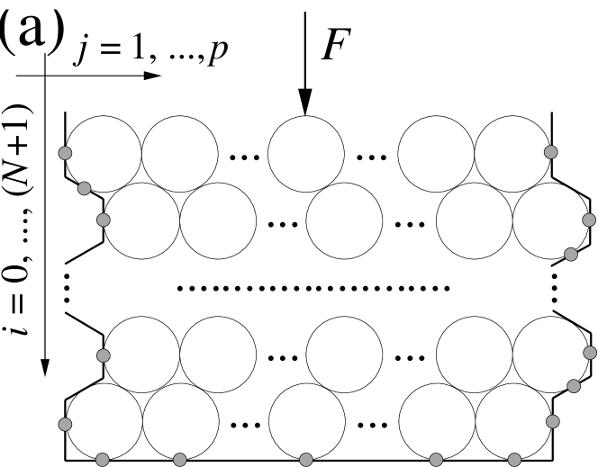
While such a method has recently been shown to produce single inter-grain force probability distributions in fixed geometry that compare well with experiments [17], in this Letter we demonstrate that it also leads to an average response function qualitatively in agreement with experiments. More precisely, we determine the behaviour of the response of a two-dimensional hexagonal packing of rigid, frictionless spherical grains placed between two vertical walls (see Fig.1), due to a vertically downward force $F$ applied on a single grain at the top layer. Experimentally [11, 12] it was found that a force $F$ applied to the top of a hexagonal packing of photo-elastic particles propagates mainly along the two downward lattice directions. We define the response of the packing as $\left[\langle W_{i,j}\rangle-\langle W_{i,j}^{(0)}\rangle\right]/F$ where $W_{i,j}$ and $W_{i,j}^{(0)}$ are the vertical force transmitted by the $(i,j)$th grain to the layer below it respectively with and without the external force $F$, and the angular brackets denote averaging over all configurations of mechanically stable contact forces with equal probability.

To start with, we describe a method for assigning the uniform probability measure on the ensemble ${\cal E}$ of stable repulsive contact forces pertaining to a fixed geometrical configuration of $P$ rigid, frictionless two-dimensional grains of arbitrary shapes and sizes (for a rigorous geometrical description of a granular packing, see Ref. [15]). The directions of the forces are fixed at each of the $Q$ contact points, and one can represent any force configuration by a column vector $\mathsf{F}$ consisting of $Q$ non-negative scalars $\{F_{k}\}$ (with ${k=1,\ldots,Q}$) as its individual elements. These elements satisfy $3P$ Newton’s equations ($3$ equations per grain: two for balancing forces in the $x$ and $y$ directions and one for balancing torque), which can be represented as ${\mathbf{A}}\cdot{\mathsf{F}}={\mathsf{F}}_{{ext}}$. Here, $\mathbf{A}$ is a $3P\times Q$ matrix, and $\mathsf{F}_{{ext}}$ is a $3P$-dimensional column vector representing the external forces. If we assume $3P<Q$ [20], then there is no unique solution for $\mathsf{F}$. Instead, there exists a whole set of solutions that can be constructed via the three following steps: (1) one first identifies an orthonormal basis $\{{\mathsf{F}}^{(l)}\}$ ($l=1,\ldots,d_{K}=Q-3P$) that spans the space of $Ker({\mathbf{A}})$; (2) one then determines a unique solution ${\mathsf{F}}^{(0)}$ of ${\mathbf{A}}\cdot{\mathsf{F}}^{(0)}={\mathsf{F}}_{{ext}}$ by requiring ${\mathsf{F}}^{(0)}.{\mathsf{F}}^{(l)}=0$ for $l=1,\ldots,d_{K}$; and (3) one finally obtains all solutions of ${\mathbf{A}}\cdot{\mathsf{F}}={\mathsf{F}}_{{ext}}$ as ${\mathsf{F}}={\mathsf{F}}^{(0)}+\sum\limits_{l=1}^{Q-3P}f_{l}\,{\mathsf{F}}^{(l)}$, where $f_{l}$ are real numbers. This implies that ${\cal E}$ is parametrized by the $f_{l}$’s belonging to a set ${\cal S}$ obeying the non-negativity conditions for all forces. The uniform measure on ${\cal E}$, which is usually compact [23], is thus equivalent to the uniform measure $d\mu=\prod\limits_{k}dF_{k}\,\delta({\mathbf{A}}\cdot{\mathsf{F}}-{\mathsf{F}_{{ext}}})\,\Theta({F_{k}})=\prod\limits_{l}df_{l}$ on ${\cal S}$.

In our model, the grains are spherical, so that the dimension of ${\mathbf{A}}$ reduces to $2P\times Q$. We consider the force $F$ and the weights of the individual grains as the non-zero elements of ${\mathsf{F}}_{{ext}}$, while ${\mathsf{F}}$ is composed of all inter-particle and non-zero boundary forces. Simple counting then shows that $Q=3Np+5p+N+2$ (see Fig. 1). The matrix ${\mathbf{A}}$ represents two equations per particle (see Fig. 1 (b-c)) [20]

$$F^{(i,j)}_{5}=F^{(i,j)}_{2}+mg/\sqrt{3}+[F^{(i,j)}_{4}-F^{(i,j)}_{3}]$$

$$F^{(i,j)}_{6}=F^{(i,j)}_{1}+mg/\sqrt{3}-[F^{(i,j)}_{4}-F^{(i,j)}_{3}]$$

$$W_{N+1,j}=\sqrt{3}\left[F^{(N+1,j)}_{1}+F^{(N+1,j)}_{2}\right]/2+mg$$

$$F^{(N+1,j)}_{4}-F^{(N+1,j)}_{3}=\left[F^{(N+1,j)}_{1}-F^{(N+1,j)}_{2}\right]/2\,,$$ (1)

i.e., $2(N+2)p$ equations all together, implying that $d_{K}=N+2+(N+1)p$. We choose $F^{(i,1)}_{3}$’s for $i\leq(N+1)$ and $F^{(i,j)}_{4}$’s for $i\leq N,1\leq j\leq N$ to parameterize ${\cal E}$. Once these forces are fixed, all the others are uniquely determined by solving Eq. (1) layer by layer from top down [24]. It is easily seen that the number of these parameters is indeed $d_{K}$, as it should be. Clearly, in this formulation, $W_{i,j}=\sqrt{3}\left[F^{(i,j)}_{1}+F^{(i,j)}_{2}\right]/2+mg$, and $d\mu=\prod\limits_{i=0}^{N+1}dF^{(i,1)}_{3}\!\!\prod\limits_{(i^{\prime},j)=(0,1)}^{(N,p)}\!\!dF^{(i^{\prime},j)}_{4}$ on ${\cal S}$ for our model. Furthermore, with $G_{i,j}=F^{(i,j)}_{4}-F^{(i,j)}_{3}$, i.e., with [24]

$$F^{(i,j)}_{4}=F^{(i,1)}_{3}+{\textstyle\sum\limits_{j^{\prime}=1}^{j}}G_{i,j^{\prime}}\,,$$ (2)

$\prod\limits_{(i,j)=(0,1)}^{(N,p)}\!\!dF^{(i,j)}_{4}$ in $d\mu$ can be replaced by $\prod\limits_{(i,j)=(0,1)}^{(N,p)}\!\!dG_{i,j}$. In this form of $d\mu$, in order to respect the non-negativity conditions for $F^{(i,j)}_{5}$’s and $F^{(i,j)}_{6}$’s, one must satisfy

$$\displaystyle{-\left[F^{(i,j)}_{2}+mg/\sqrt{3}\right]\leq G_{i,j}\leq F^{(i,j)}_{1}+mg/\sqrt{3}}\,,$$ (3)

implying that the set ${\cal S^{\prime}}$ of allowed values of $G_{i,j}$’s is compact. However, since the non-negativity conditions for $F^{(i,j)}_{3}$ and $F^{(i,j)}_{4}$’s provide only lower bounds for $F^{(i,1)}_{3}$’s, ${\cal S}$ in this model is actually unbounded.

Figure 2: Colour plots for $N=35$ and $m=0$: (a) mean response; (b) the standard deviation of the response.

Figure 3: Behavior of $\langle W(i,j)\rangle$ for $m=0$ in reduced co-ordinates $x$ and $z$: (a) scaling of $\langle W(x,z)\rangle$ with system size for $|x|<z/2$ at two $z$ values (for clarity, $z=0.8$ and $z=0.6$ have been shifted upwards by one and two units respectively); (b) data collapse for $\langle W(x,z)\rangle|_{x=z/2}$ at three $N$ values. See text for further details.

The remedy we use is to fix the $F^{(i,1)}_{3}$ values: indeed, as can be seen in Eq. (1), the values of the $W_{i,j}$ depend only the $G_{i,j}$’s so that in this model the precise values of $F^{(i,1)}_{3}$ have no physical meaning. Nevertheless, one has to be careful: notice that the $G_{i,j}$’s are differences of the physical contact forces and thus they are allowed to become negative in magnitude. In fact, Eqs. (2) and (3) together imply that if $F^{(i,1)}_{3}<2[F+(i-1)mg]/\sqrt{3}$, then the positivity requirement of the $F^{(i,j)}_{4}$ might further restrict the choice of $G_{i,j}$ values within the bounds of inequality (3). In this Letter, we fix the magnitudes $F^{(i,1)}_{3}=2[F+(i-1)mg]/\sqrt{3}\equiv F_{0}$ so that all values of $G_{i,j}$ within the bounds of inequality (3) are allowed (details of the cases $F^{(i,1)}_{3}<F_{0}$ appear elsewhere [18, 19]) This arrangement reduces the uniform measure over ${\cal E}$ to the uniform measure on ${\cal S^{\prime}}$, which is a $(N+1)p$-dimensional polyhedron.

To evaluate $\langle W_{i,j}\rangle=\displaystyle{\frac{1}{{\cal N}}\int}_{\!\!\cal S^{\prime}}\,W_{i,j}\prod_{kl}dG_{k,l}$, where ${\cal N}=\int_{{\cal S}^{\prime}}\prod_{ij}dG_{i,j}$ is the normalization constant, we define

$$q_{i,j}=\left[\sqrt{3}(G_{i,j}+F^{(i,j)}_{2})/2+mg/2\right]/W_{i,j}\,,$$ (4)

where $q_{i,j}$ is the fraction of $W_{i,j}$ that the $(i,j)$th particle transmits to the layer below it toward the left, i.e., $F^{(i,j)}_{5}=2q_{i,j}W_{i,j}/\sqrt{3}$ and $F^{(i,j)}_{6}=2(1-q_{i,j})W_{i,j}/\sqrt{3}$. Equation (4) then reduces Eq. (3) to $0\leq q_{i,j}\leq 1$. Clearly, $W_{0,j}$ are the external forces applied on the top layer. For $i>0$, $W_{i,j}$ is a function of $q_{k,l}$ for $k<i$, since

$$W_{i,j}=(1-q_{i-1,j-1})\,W_{i-1,j-1}+q_{i-1,j}\,W_{i-1,j}+mg.$$ (5)

It may seem from Eq. (5) that in the hexagonal geometry of Fig. 1, one simply recovers the $q$-model [5]. There is however an important subtlety to take notice of. In the $q$-model, the $q$’s corresponding to different grains are usually uncorrelated, while in our case, the uniform measure on ${\cal S}^{\prime}$ implies, from Eq. (4), that

$$\textstyle{\prod\limits_{i,j}}\,dG_{i,j}=2^{(N+1)p}\,\textstyle{\prod\limits_{i,j}}dq_{i,j}\,W_{i,j}(q)\big{/}3^{(N+1)p/2}\,.$$ (6)

Due to the presence of the Jacobian on the right hand side of Eq. (6), the uniform measure on ${\cal S^{\prime}}$ translates to a non-uniform measure on the $(N+1)p$-dimensional unit cube formed by the accessible values of the $q$’s.

Notice an important artifact of this approach: the joint probability distribution $\prod\limits_{i,j}W_{i,j}(q)$ depends on the $q_{i,j}$ values over the whole system, thereby making $q_{i,j}$’s correlated with each other. In fact, the induced probability $P(q_{i,j})$ for a single grain does not only depend on the number of layers present above the grain, but also on the number of layers below it. It is thus clear that the forces in this model do not propagate top down, as they do in hyperbolic “stress-only” models [2].

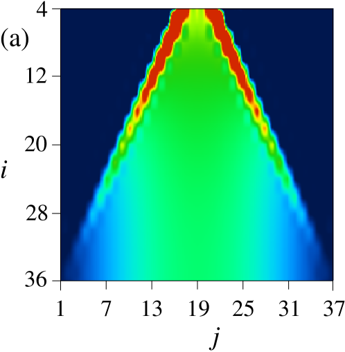
For massless grains ($m=0$), it is clear that (i) for $F=0$, $W_{ij}^{(0)}=0\,\forall(i,j)$ (ii) the $\langle W_{i,j}\rangle$ values scale linearly with $F$ (hence, we use $F=1$), and (iii) $\langle W_{i,j}\rangle=0$ outside the triangle formed by the two downward lattice directions emanating from $(i,j)=(0,j_{0})$, the point of application of $F$. The $\langle W_{i,j}\rangle$’s, evaluated numerically via the Metropolis algorithm on these $q$’s, appear in Fig. 3.

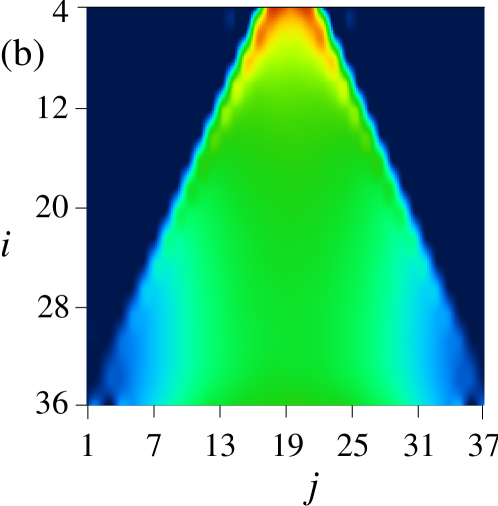
Our simulation results for $\langle W_{i,j}\rangle$ and the standard deviation $\delta W_{i,j}=\sqrt{\langle W^{2}_{i,j}\rangle-\langle W_{i,j}\rangle^{2}}$ within the triangle are plotted in Fig. 2, using the built-in cubic interpolation function of Mathematica. Outside the triangle, $\langle W_{i,j}\rangle\equiv 0$ appears in deep indigo; the largest $\langle W_{i,j}\rangle$ value within the triangle appears in dark red; and any other non-zero $\langle W_{i,j}\rangle$ value is represented by a linear wavelength scale in between [25]. We find $\forall N$ that (a) the $\langle W_{i,j}\rangle$ values display two single-grain-diameter-wide symmetric peaks that lie precisely on the two downward lattice directions emanating from $j_{0}$, (b) the magnitudes of these peaks decrease with depth, and (c) only a central maximum for $\langle W_{i,j}\rangle$ is seen at the very bottom layer ($i=N+1$). The standard deviation $\delta W_{ij}$ has a similar shape to $\langle W_{i,j}\rangle$, although the peaks are less pronounced.

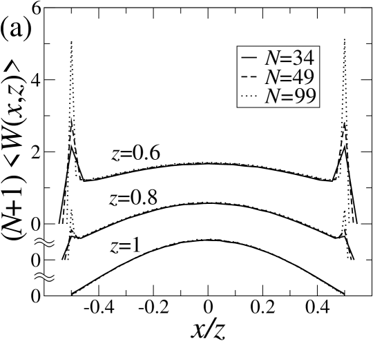
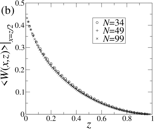
We further define $x=(j-j_{0})/(N+1)$ and $(j-j_{0}+1/2)/(N+1)$ respectively for even and odd $i$, and $z=i/(N+1)$ [see Fig. 1] in order to put the vertices of the triangle formed by the locations of non-zero $\langle W_{i,j}\rangle$ values on $(0,0),(-1/2,1)$ and $(1/2,1)\,\,\forall N$. The excellent data collapse shown in Fig. 3 indicates that the $\langle W_{i,j}\rangle$ values for $|x|<z/2$ scale with the inverse system size [Fig. 3(a); we however show only three $z$ values], while the $\langle W_{i,j}\rangle$ values for $|x|=z/2$ lie on the same curve for all system sizes [Fig. 3(b)]. The data suggest that in the thermodynamic limit $N\rightarrow\infty$, the response field $\langle W(x,z)\rangle$ scales $\sim 1/N$ for $|x|<z/2$, but reaches a non-zero limiting value on $|x|=z\,\,\forall z<1$. We thus expect $\lim\limits_{N\rightarrow\infty}\langle W(x,z)\rangle\big{|}_{|x|=z/2}>\langle W(x,z)\rangle\big{|}_{|x|<z/2}\,\,\forall z<1$; or equivalently, a double-peaked response field at all depths $z<1$ for large $N$.

We have not found a simple explanation for such scaling behaviour of $\langle W(x,z)\rangle$. It however turns out that exact analytical expressions can be obtained for all moments of $W_{i,j}\,\,\forall(i,j)$, for any $N$. The detailed calculations appear in Ref. [18].

Figure 4: Scaling properties of $\langle w(x,z)\rangle$, analogous to Figs. 3(b-c), for $\beta=100$ and three $N$ values (a.u.$\,\equiv\,$arbitrary units).

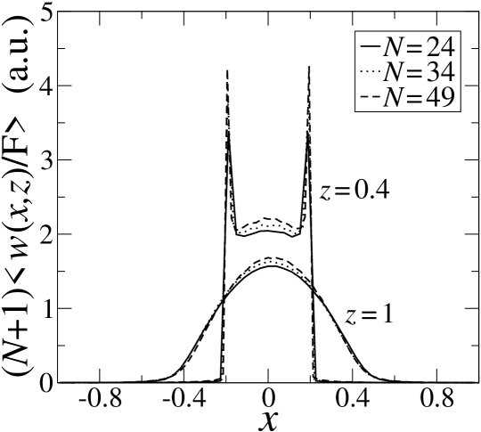
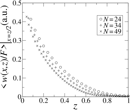
In view of the self-similarity of $\langle W(x,z)\rangle$ that we observe for different system sizes in Figs. 3(b-c), it seems natural that we also study the same properties for $m\neq 0$. In this case, $\langle W_{i,j}^{(0)}\rangle\neq 0$ and $\langle W_{i,j}\rangle\not\propto F$. To minimize the effect of the boundaries in the regions around $j=j_{0}$, we have used $p=2N+5$. For $m\neq 0$, the relevant scale for the magnitude of $F$ is obviously $\alpha=F/mg$. For $\alpha\neq 0$, just like in the case of $m=0$, we observe a double-peaked response, and the peaks are still single grain diameter wide. Furthermore, for a given value of $N$ and increasing $\alpha$, the magnitude of the response on $x=z/2$ decays more slowly, i.e. the peaks penetrate the packing to progressively higher values of $z$. In order to avoid repetition, we do not use colour figures like Fig. 3(a) to demonstrate this behaviour, but the trend of the data clearly indicates that for fixed $N$, one should recover the results corresponding to $m=0$ in the limit $\alpha\rightarrow\infty$.

It is clear from the qualitative behaviour described in the above paragraph that in order to obtain scaling with increasing $N$, one also needs to scale $\alpha$ in some way. To this end, we define $\beta=\alpha/(N+1)$ and keep $\beta$ constant for increasing $N$. The corresponding graphs are shown in Fig. 4 for $\beta=100$. The fact that the self-similarity in Fig. 4 for different system sizes is not as striking as in Figs. 3(b-c) suggests that there is more to the story of scaling properties. It is likely that the full scaling properties can be unraveled only at much higher values of $N$, but unfortunately, simulations with $N$ values significantly higher than $50$ require impractically long times.

In summary, we find that assigning equal probability to all mechanically stable force configurations for rigid, frictionless spherical grains (with or without mass) in a two-dimensional hexagonally close-packed geometry yields a double-peaked response. The peaks are single grain diameter wide, they lie on the two downward lattice directions emanating from the point of application of $F$. With increasing depth, the magnitude of the peaks decreases, and a third peak starts to develop directly below the applied force. Near (and on) the bottom layer only the middle peak persists; i.e., the response becomes single-peaked. As the number of layers is increased, the transition from double to single peak takes place deeper in the packing. Moreover, for grains each with mass $m$, the peaks penetrate the packing deeper with larger $F$. The standard deviation of the response is similar in shape to the response, but the peaks are weaker.

We emphasize that the results presented here are obtained for the boundary condition $F^{(i,1)}_{3}\geq F_{0}$. The case $F^{(i,1)}_{3}<F_{0}$ and other kinds of boundary conditions have been analyzed elsewhere [18, 19]. These results together indicate that the quantitative behaviour of the response depends crucially on the side forces (i.e. boundary conditions) — this feature is consistent with other theoretical approaches [7]. In particular, we note that the transition to a single-peaked response does not take place for $F^{(i,1)}_{3}$ sufficiently small.

We also note that the double-peaked structure of both the mean response and the standard deviation of the response is in qualitative agreement with experiments [11, 12, 13], but the fluctuations observed in the model are much weaker than found in experiments [12]. Another crucial difference between our and the experimental results is that in this model the peaks are single-diameter wide, while in experiments the peaks widen with depth [12]. This difference probably stems from the fact that in experiments the effect of inter-grain friction can never be neglected. Presence of friction would also certainly make fluctuations in the response $\delta W_{i,j}$ stronger. A study of the effects of friction on the response along the lines of [26] is therefore an important direction for future work.

It is a pleasure to thank J.-P. Bouchaud, D. Dhar, J. M. J. van Leeuwen, B. Nienhuis, J. Snoeijer and D. Wolf for useful discussions. Financial support was provided by the Dutch research organization FOM (Fundamenteel Onderzoek der Materie).

References

- [1] H. M. Jaeger et al., Rev. Mod. Phys. 68, 1259 (1996); P. G. de Gennes, Rev. Mod. Phys. 71, 374 (1999).
- [2] J.-P. Bouchaud, in Les Houches, Session LXXVII, J.L. Barrat et al. Eds., Springer-EDP Sciences (2003). See also references cited therein.
- [3] L. Vanel et al., Phys. Rev. E 60, R5040 (1999).
- [4] D. M. Mueth et al, Phys. Rev. E 57, 3164 (1998); D. L. Blair et al, Phys. Rev. E 63, 041304 (2001); F. Radjai et al Phys. Rev. Lett. 77, 274 (2001).
- [5] S. N. Coppersmith et al., Phys. Rev. E 53, 4673 (1996).
- [6] R. M. Nedderman, Statics and Kinematics of Granular Materials, Cambridge University Press (1982).
- [7] C. Goldenberg et al., Phys. Rev. Lett. 89, 084302 (2002); I. Goldhirsch et al., Eur. Phys. J. E 9, 245 (2002).
- [8] G. Reydellet and E. Clément, Phys. Rev. Lett. 86, 3308 (2001).
- [9] D. Serero et al., Eur. Phys. J. E 6, 169 (2001).
- [10] A. Atman et al., cond-mat 0501118.
- [11] J. Geng et al., Phys. Rev. Lett. 87, 035506 (2001).
- [12] J. Geng et al., Physica D 182, 274 (2003).
- [13] N. W. Mueggenburg et al., Phys. Rev. E 66, 031304 (2002).
- [14] S. F. Edwards et al., Physica A 157, 1080 (1989).
- [15] S. F. Edwards et al., Physica A 302, 162 (2001).
- [16] H. A. Makse et al., Nature 415, 614 (2002).
- [17] J. H. Snoeijer et al., Phys. Rev. Lett. 92, 054302 (2004).
- [18] S. Ostojic and D. Panja, J. Stat. Mech.(JSTAT) P01011 (2005).
- [19] S. Ostojic and D. Panja, proceedings of Powders and Grains 2005, cond-mat/0503752.
- [20] For frictionless rigid spherical grains, the number of forces is exactly equal to the number of equations [21]. Numerical studies [22] however find that in the limit of large but finite rigidity the number of equations is always less then the number of contacts, and this is what we assume here.
- [21] C. F. Moukarzel, Phys. Rev. Lett. 81, 1634 (1998); A. V. Tkachenko et al., Phys. Rev. E 60, 687 (1999).
- [22] L. E. Silbert et al., Phys. Rev. E 65, 031304 (2002).
- [23] T. Unger et al., cond-mat/0403089.
- [24] One uses the fact that for .
- [25] The thin green regions that appear on the outer edge of the triangle are artifacts of the interpolation. It is also important to note that the horizontal forces are non-zero everywhere, but they are not shown in Fig. 3(a).
- [26] L. Breton et al., Europhys. Lett. 60, 813 (2002).