Phase diagram and quasiparticle properties of the Hubbard model within cluster two-site DMFT

Abstract

We present a cluster dynamical mean-field treatment of the Hubbard model on a square lattice to study the evolution of magnetism and quasiparticle properties as the electron filling and interaction strength are varied. Our approach for solving the dynamical mean-field equations is an extension of Potthoff’s “two-site” method [Phys. Rev. B. 64, 165114 (2001)] where the self-consistent bath is represented by a highly restricted set of states. As well as the expected antiferromagnetism close to half-filling, we observe distortions of the Fermi surface. The proximity of a van Hove point and the incipient antiferromagnetism lead to the evolution from an electron-like Fermi surface away from the Mott transition, to a hole-like one near half-filling. Our results also show a gap opening anisotropically around the Fermi surface close to the Mott transition (reminiscent of the pseudogap phenomenon seen in the cuprate high-$T_{c}$ superconductors). This leaves Fermi arcs which are closed into pockets by lines with very small quasiparticle residue.

I Introduction

Understanding the physics of the Hubbard model continues to be a fundamental issue in strongly correlated systems. This model captures the transition between a metallic state and a correlated insulator; how this transition takes place has been investigated by many workers in the past, with differing approaches emphasizing the formation of Hubbard bands, hubbard_1964a the increasing mass of the quasiparticles brinkman_1970a and the proximity to antiferromagnetism. slater_1951a Significant progress has been made in recent years by the development of dynamical mean-field theory (DMFT). georges_1996a Here a set of equations—exact in the limit of infinite dimensions—is derived which maps the problem onto an interacting impurity model to be solved self-consistently. This method has revealed a Mott transition that is a synthesis of the pictures of Mott and Brinkman–Rice: formation of Hubbard bands in parallel with a large mass quasiparticle. The absence of momentum dependence in correlations within DMFT means that this method does not account for variations in quasiparticle properties across the Brillouin zone. This is likely to be important if the Mott transition has an antiferromagnetic aspect.

Building on the success of dynamical mean-field theory, extensions to the theory are being actively studied. One such extension combines it with density-functional theory to improve the treatment of local correlations. anisimov_1997a ; lichtenstein_1998a ; lichtenstein_2001a Another considers intersite correlations via so called cluster DMFT. hettler_1998a ; kotliar_2001a ; lichtenstein_2000a It is also often important to include multiple local orbitals when modeling real materials such as the correlated oxides. In all of these extensions the task of solving the resulting self-consistent equations becomes increasingly problematic: the equations require the solution of impurity models with an increasing number of local degrees of freedom, which often demand high-performance computing resources and sophisticated approximation schemes to extract the low energy physics.

Yet in contrast to these computationally intensive approaches, Potthoff potthoff_2001a demonstrated that much of the Mott transition physics could be captured with a drastic approximation of the non-interacting bath of electrons that couples to the impurity in DMFT. Whereas in one computational scheme for tackling the DMFT equations, the bath is modeled by up to twelve coupled sites (the exact diagonalization method caffarel_1994a ), Potthoff used just a single site to represent the bath. The self-consistency conditions were constructed to ensure that the quasiparticle properties and band filling were matched. Solving them yielded a successful description of the Mott transition showing, for example, the narrowing of the quasiparticle resonance and the formation of the Hubbard bands. A value of the critical Hubbard interaction, $U$, was obtained comparable to the best calculations.

In this paper we present an extension of Potthoff’s “two-site” approach to treat cluster DMFT. We use our method to investigate the approach to the Mott transition for a single band Hubbard model on a two-dimensional square lattice with nearest neighbor hopping, $t$. The Hamiltonian is

$$\hat{H}_{\rm Hub}=\sum_{{{\bm{\mathrm{k}}}},\sigma}\epsilon^{\vphantom{\dagger}}_{{\bm{\mathrm{k}}}}\hat{c}^{\dagger}_{{{\bm{\mathrm{k}}}},\sigma}\hat{c}^{{\vphantom{\dagger}}}_{{{\bm{\mathrm{k}}}},\sigma}+U\sum_{i}\hat{c}^{\dagger}_{i\uparrow}\hat{c}^{{\vphantom{\dagger}}}_{i\uparrow}\hat{c}^{\dagger}_{i\downarrow}\hat{c}^{{\vphantom{\dagger}}}_{i\downarrow}\;,$$ (1)

where $\epsilon_{{\bm{\mathrm{k}}}}=-2t[\cos(k_{x}a)+\cos(k_{y}a)]$. We study this model as an example case, although our method is readily extended to more complicated Hamiltonians. The method allows us to quickly investigate the zero temperature phase diagram across a large range of parameter space using a desktop computer. The efficacy of our approach is reinforced by our results which are consistent with other results in the literature for the magnetic phase diagram. Moreover we can go beyond existing work to study the quasiparticle properties in momentum space: seeing, for example, how an electron-like metal (well away from half-filling) becomes a hole-like doped Mott insulator near half-filling. Some of our results are suggestive of the physics of the cuprate superconductors with the appearance of pseudogap regions and “arc-like” Fermi surfaces brought about, in our case, by the combination of antiferromagnetism and proximity to a van Hove point. We also observe a Fermi surface distortion resulting from a Pomeranchuk instability also reported elsewhere in the literature.halboth_2000a ; hankevych_2002a ; metzner_2003a ; neumayr_2003a Physically, this is due to the proximity of the Fermi surface to the van Hove point, but the tendency will be exaggerated in our model due to the reduced symmetry of our cluster (see later).

We begin with a summary of DMFT together with Potthoff’s “two-site” approach. We then discuss how DMFT can be extended to a cluster of sites, and describe our application of Potthoff’s approach to a cluster consisting of a pair of sites. We then demonstrate this method on the 2D Hubbard model and present our results. We conclude with a discussion of the physics behind these results and future extensions of our method.

II From DMFT to the two-site approach

The DMFT procedure georges_1996a can be described as follows. We focus on a single site of the Hubbard model, and notionally integrate out all the other sites. This gives an effective action for the remaining site of the form

$$\begin{split}S_{\text{eff}}=&-\int_{0}^{\beta}d\tau\int_{0}^{\beta}d\tau^{\prime}c_{\sigma}^{\dagger}(\tau)\mathcal{G}^{-1}_{0}(\tau-\tau^{\prime})c_{\sigma}^{{\vphantom{\dagger}}}(\tau^{\prime})\\ &+U\int_{0}^{\beta}d\tau c^{\dagger}_{\uparrow}(\tau)c^{\vphantom{\dagger}}_{\uparrow}(\tau)c^{\dagger}_{\downarrow}(\tau)c^{\vphantom{\dagger}}_{\downarrow}(\tau).\end{split}$$ (2)

The function $\mathcal{G}_{0}$ completely encapsulates the dynamics of electrons entering and leaving the site from the rest of the lattice; however it is not known a priori since we cannot in practice integrate out the other sites. With this action we could determine the interacting Green’s function $G_{\text{local}}(i\omega_{n})$, and extract a local self-energy from the Dyson’s equation

$$G_{\text{local}}^{-1}(i\omega_{n})=\mathcal{G}_{0}^{-1}(i\omega_{n})-\Sigma_{\text{local}}(i\omega_{n}).$$ (3)

The DMFT ansatz, exact in infinite dimensions, is to use this local self-energy as a spatially homogeneous (but frequency-dependent) self-energy for the full lattice problem:

$${G_{\text{lat}}(i\omega_{n},{\bm{\mathrm{k}}})}^{-1}=i\omega_{n}+\mu-\epsilon_{{\bm{\mathrm{k}}}}-\Sigma_{\text{local}}(i\omega_{n}).$$ (4)

The self-consistency requirement that the on-site Green’s function of the extended lattice (containing the self-energy) is the same as the local Green’s function we started with, i.e.

$$G_{\text{local}}(i\omega_{n})=\sum_{{\bm{\mathrm{k}}}}G_{\text{lat}}(i\omega_{n},{\bm{\mathrm{k}}}),$$ (5)

provides the constraint on the unknown initial function $\mathcal{G}_{0}(i\omega_{n})$, thereby completing the self-consistency loop.

Eq. 2 is the effective action of a single interacting impurity coupled to a continuum bath, but the procedure described above cannot be achieved exactly because the single site impurity problem with an unrestricted bath is still intractable. One must approximate and use a model that is practically solvable; for example, a finite-sized impurity model for exact diagonalization, caffarel_1994a or a discretized effective action for Quantum Monte Carlo methods. jarrell_1992a This means that only limited functional forms of $\mathcal{G}_{0}(i\omega_{n})$ can be represented, and also that the final self-consistency condition cannot be implemented precisely.

In the “two-site” realization of DMFT introduced by Potthoff, potthoff_2001a the local model is an impurity site together with a bath consisting of a single site only, with a Hamiltonian:

$$\hat{H}=U\hat{a}^{\dagger}_{\uparrow}\hat{a}^{\vphantom{\dagger}}_{\uparrow}\hat{a}^{\dagger}_{\downarrow}\hat{a}^{\vphantom{\dagger}}_{\downarrow}+\sum_{\sigma}\epsilon_{c\sigma}\hat{c}^{\dagger}_{\sigma}\hat{c}^{\vphantom{\dagger}}_{\sigma}+V_{\sigma}(\hat{a}^{\dagger}_{\sigma}\hat{c}^{\vphantom{\dagger}}_{\sigma}+\hat{c}^{\dagger}_{\sigma}\hat{a}^{\vphantom{\dagger}}_{\sigma})-\mu\hat{a}^{\dagger}_{\sigma}\hat{a}^{\vphantom{\dagger}}_{\sigma},$$ (6)

where the electron creation operators $\hat{a}^{\dagger}_{\sigma}$ and $\hat{c}^{\dagger}_{\sigma}$ are for the impurity site and the bath site respectively. Diagonalizing the non-interacting ($U=0$) model yields $\mathcal{G}_{0}(\omega)=\omega+\mu-[V_{\sigma}^{2}/(\omega-\epsilon_{c\sigma})]$ (where we are now considering zero temperature real frequency Green’s functions). The two-site model allows a minimal frequency dependence in $\mathcal{G}_{0}$. By exactly diagonalizing the many particle Hamiltonian of Eq. 6, the local on-impurity-site interacting Green’s function $G_{\text{imp}}(\omega)$ can be constructed from the Lehmann representation, and the self-energy $\Sigma(\omega)$ is extracted (c.f. Eq. 3) using:

$$G_{\text{imp},\sigma}^{-1}(\omega)=\omega+\mu-\frac{V_{\sigma}^{2}}{\omega-\epsilon_{c\sigma}}-\Sigma_{\text{local},\sigma}(\omega).$$ (7)

The full functional self-consistency of Eq. 5 cannot be achieved within such a restricted representation so it is necessary to decide how best to implement a self-consistency requirement. Potthoff chose two physically motivated features, taking advantage of the analytic simplicity of the two-site impurity model. Firstly, the electron fillings given by the Green’s functions must be equal for the impurity model and the lattice model. Secondly, features of the central quasiparticle peak are matched: the self-energy is reduced to the low energy form $\Sigma_{\text{local},\sigma}(\omega)\sim a_{\sigma}+b_{\sigma}\omega$, and terms of the resulting “coherent” impurity and lattice Green’s functions at high energy are matched (see Ref. potthoff_2001a, for more detail). In effect, the shape of the central quasiparticle peak is analyzed by the size of its high energy tails, isolated from other parts of the spectrum. The resulting self-consistency conditions for the four bath parameters ($V_{\sigma},\epsilon_{c\sigma}$) are:

$$n_{\text{imp},\sigma}=n_{\text{lat},\sigma}\qquad\text{and}\qquad V_{\sigma}^{2}=\sum_{{\bm{\mathrm{k}}}}\epsilon_{{\bm{\mathrm{k}}}}^{2}z_{\sigma}\;,$$ (8)

where the quasiparticle residue

$$z_{\sigma}=\left(1-\frac{d\Sigma_{\text{local},\sigma}}{d\omega(0)}\right)^{-1}=\frac{1}{(1-b_{\sigma})}\;,$$ (9)

and we have assumed that $\sum_{{\bm{\mathrm{k}}}}\epsilon_{{\bm{\mathrm{k}}}}=0$.

Solving these equations produces results for the Mott transition which compare well with the full DMFT, and properties of the Fermi liquid which are consistent with exact results (see Ref. potthoff_2001a, ). It is hard to imagine a simpler model which can do this; it succeeds because of the physical motivation of its self-consistency conditions, namely the filling and properties of the quasiparticle peak. It is a useful approach for calculations on extended models such as multiple bands koga_2004a and, as we shall demonstrate, clusters.

III From cluster DMFT to two-site pair-cluster DMFT

We now consider an extension of this method to cluster DMFT: hettler_1998a ; kotliar_2001a instead of starting with a single site, self-consistency conditions are derived for a cluster of sites, which allows a momentum dependence in the self-energy. The geometry of the lattice becomes important and hence different types of magnetic order can be investigated, and spectral information varies non-trivially in ${\bm{\mathrm{k}}}$-space, unlike conventional DMFT. A number of studies have been reported. lichtenstein_2000a ; huscroft_2001a ; maier_2002a ; dahnken_2003a ; parcollet_2003a We describe here a cluster DMFT for the case where the cluster consists of just a pair of sites.

We then detail how to implement Potthoff’s two-site method to solve cluster DMFT. This can be contrasted with the exact diagonalization formulation of conventional DMFT, caffarel_1994a where a single impurity site with multiple bath sites is used; instead, we use multiple impurity sites in a cluster and include correlations in the simplest way via Potthoff’s scheme for single bath sites. Below, we derive the self-consistency conditions for the pair-cluster (each of the two cluster sites is connected to a single bath site).

Implementing a cluster DMFT is fundamentally ambiguous, as recently noted by Biroli et al.; biroli_2003a the approach we adopt is “CDMFT” within their classification, which is arguably the simplest scheme appropriate for broken symmetry states. One of the strengths of conventional DMFT is that it is exact in the limit of infinite dimensions. In contrast, our cluster approach is not a systematic $1/d$ correction, though it is of course exact in the limit of infinite cluster size when the self-consistent bath is merely a sophisticated boundary condition. hettler_1998a

In cluster DMFT we imagine integrating out all sites except those in the cluster. An electron can in general now leave from and arrive back at any of the sites within the cluster: the function $\mathcal{G}_{0}$ must become a matrix, coupling together the dynamics of the cluster sites. The resulting action (c.f. Eq. 2) is:

$$\begin{split}S_{\text{eff}}=&-\int_{0}^{\beta}\!d\tau\int_{0}^{\beta}d\tau^{\prime}\sum_{i,j\in\{A,B\}}c_{i\sigma}^{\dagger}(\tau)\mathcal{G}^{-1}_{0,ij}(\tau-\tau^{\prime})c_{j\sigma}^{{\vphantom{\dagger}}}(\tau^{\prime})\\ &+U\int_{0}^{\beta}d\tau\sum_{i\in\{A,B\}}c^{\dagger}_{i\uparrow}(\tau)c^{\vphantom{\dagger}}_{i\uparrow}(\tau)c^{\dagger}_{i\downarrow}(\tau)c^{\vphantom{\dagger}}_{i\downarrow}(\tau)\;,\end{split}$$ (10)

where the summations are over the cluster sites. Solving this local problem now yields a matrix $G_{\text{local},ij}$ and a matrix self-energy.

Different approaches to cluster DMFT involve different ways of combining the matrix self-energy with the non-interacting lattice Green’s function, and different self-consistency conditions. We shall now describe our particular approach, for the specific case of a 2D square lattice with a cluster consisting of a pair of sites. The sites represent the two sublattices of the bipartite square lattice, and we label them $A$ and $B$. The impurity model consists of a pair of sites connected by a $-t$ hopping element, cut out of the original lattice [see Fig. 1(a)]. Each site has its own independent bath site [Fig. 1(b)]. The Hamiltonian for this pair-cluster impurity model is diagonalized as previously, resulting in a $2\times 2$ matrix Green’s function, whose self-energy matrix is extracted (c.f. Eq. 7) using Dyson’s equation:

$${\bm{G}}_{\text{imp},\sigma}^{-1}(\omega)=\begin{pmatrix}\omega+\mu-\frac{V_{A\sigma}^{2}}{\omega-\epsilon_{cA,\sigma}}-\Sigma_{A\sigma}(\omega)&t-\Sigma_{AB,\sigma}(\omega)\\ t-\Sigma_{AB,\sigma}(\omega)&\omega+\mu-\frac{V_{B\sigma}^{2}}{\omega-\epsilon_{cB,\sigma}}-\Sigma_{B\sigma}(\omega)\end{pmatrix}\;,$$ (11)

where the matrix index is the cluster site $(A,B)$.

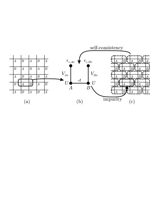
Figure 1: In our pair-cluster approach we identify a small cluster in the lattice (a), and treat this cluster as an “impurity” connected to a bath. A highly truncated basis is chosen for this bath, leading to an impurity model with four sites (b). To reconstruct the extended system, the cluster is re-embedded in the lattice periodically (c). The bath is then adjusted to ensure it is self-consistent with this embedding. Although our cluster shape manifestly breaks the $x$-$y$ symmetry, there are self-consistent solutions which reflect the original square lattice symmetry.

The non-interacting lattice Green’s function now has ${\bm{\mathrm{k}}}$-dependence from the Fourier transform of hopping elements to surrounding clusters [Fig. 1(c)], and is a matrix with respect to the cluster sites $(A,B)$. Combining it with the matrix self-energy from the impurity model according to the DMFT ansatz, gives the interacting lattice Green’s function (as above, c.f. Eq. 4):

$${\bm{G}}_{\text{lat},\sigma}^{-1}(\omega,{\bm{\mathrm{k}}})=\begin{pmatrix}\omega+\mu-\Sigma_{A\sigma}(\omega)&-\epsilon_{{\bm{\mathrm{k}}}}e^{ik_{x}a}-\Sigma_{AB,\sigma}(\omega)\\ -\epsilon_{{\bm{\mathrm{k}}}}e^{-ik_{x}a}-\Sigma_{AB,\sigma}(\omega)&\omega+\mu-\Sigma_{B\sigma}(\omega)\end{pmatrix}.$$ (12)

Full self-consistency would require that the matrix version of Eq. 5 be satisfied, but here because of the restricted representation of $\mathcal{G}_{0,ij}$ using just two additional non-interacting sites, we must adopt a more modest self-consistency requirement. We generalize the approach of Ref. potthoff_2001a, and require firstly that the filling of each sublattice is the same for the impurity and lattice models:

$$n_{\text{imp},\{A,B\},\sigma}=n_{\text{lat},\{A,B\},\sigma}\;,$$ (13)

which will effectively constrain $\epsilon_{c,\{A,B\},\sigma}$. The second condition characterizes the coherent quasiparticle peak. Expanding the Green’s function matrices at high $\omega$, with the coherent form of the self-energy in place, gives a matrix equation self-consistency equation involving a quasiparticle residue matrix ${\bm{Z}}=({\bm{I}}-d{\bm{\Sigma}}/d\omega(0))^{-1}$:

$$\begin{split}&\begin{pmatrix}\mu&t\\ t&\mu\end{pmatrix}{\bm{Z}}\begin{pmatrix}\mu&t\\ t&\mu\end{pmatrix}+\begin{pmatrix}V^{2}_{A\sigma}&0\\ 0&V^{2}_{B\sigma}\end{pmatrix}\\ =&\sum_{{\bm{\mathrm{k}}}}\begin{pmatrix}\mu&-\epsilon_{{\bm{\mathrm{k}}}}e^{ik_{x}a}\\ -\epsilon_{{\bm{\mathrm{k}}}}e^{ik_{x}a}&\mu\end{pmatrix}{\bm{Z}}\begin{pmatrix}\mu&-\epsilon_{{\bm{\mathrm{k}}}}e^{ik_{x}a}\\ -\epsilon_{{\bm{\mathrm{k}}}}e^{ik_{x}a}&\mu\end{pmatrix}\;.\end{split}$$ (14)

After the ${\bm{\mathrm{k}}}$-sum has been carried out we obtain the self-consistency condition:

$$\begin{pmatrix}V^{2}_{A\sigma}&0\\ 0&V^{2}_{B\sigma}\end{pmatrix}=\begin{pmatrix}3t^{2}Z_{B\sigma}&0\\ 0&3t^{2}Z_{A\sigma}\end{pmatrix}\;.$$ (15)

This constrains $\{V_{A},V_{B}\}$ in terms of the quasiparticle residues ${\bm{Z}}$ calculated from the local self-energy.

IV Calculations

We now describe the implementation of our cluster DMFT approach. The eight self-consistent equations (Eqs 13 and 15) are solved for the eight bath parameters $\epsilon_{c,\{A,B\},\sigma},V_{\{A,B\},\sigma}$, and additionally we wish to consider a given total filling $n$, and this provides a ninth condition which constrains the chemical potential $\mu$ such that $\sum n_{\{A,B\},\sigma}=n$. The practical problem is thus nine-dimensional root finding, for which we use a Broyden method combined with line searches. press_1992a

The two main computations are diagonalizing the Hamiltonian and calculating the band filling for the lattice case. For the latter, we sum the imaginary part of the lattice Green’s function (Eq. 12) over a finite number of points in ${\bm{\mathrm{k}}}$-space and then integrate numerically for $\omega:(-\infty,0)$. A small analytic continuation $\omega-i\delta$ is required, with $\delta\sim 0.005t$, and typically the ${\bm{\mathrm{k}}}$-sum involves $K=120$ points across the Brillouin zone; checks were done to ensure that dependence on $\delta$ and $K$ is insignificant. Fillings above $n=0.98$ are ignored since the ${\bm{\mathrm{k}}}$-space resolution is insufficient to give an accurate representation of the Fermi surface, except at exactly half-filling where this is not an issue.

For each choice of $(U,n)$ there is in general more than one set of bath parameters which satisfies the self-consistency conditions. Phases with paramagnetic, ferromagnetic, antiferromagnetic, ferrimagnetic, insulating and charge-ordered character have all emerged. We did not consider superconducting order. A pitfall of any self-consistency scheme is the production of unphysical excited states, and an advantage of the two-site DMFT is the ease of calculating the energy of a solution. Using Fetter and Walecka, fetter_1971a the energy of a fully interacting system is

$$\int_{-\infty}^{0}d\omega\sum_{{\bm{\mathrm{k}}}}\frac{1}{\pi}\underset{\omega\rightarrow\omega-i\delta}{\text{Im}}\text{tr}\left[\left({\bm{H}}_{0}(\omega,{\bm{\mathrm{k}}})+\frac{1}{2}{\bm{\Sigma}}(\omega)\right)\cdot{\bm{G}}_{\text{lat}}(\omega,{\bm{\mathrm{k}}})\right],$$ (16)

where ${\bm{H}}_{0}$ (the non-interacting Hamiltonian), ${\bm{\Sigma}}$ and ${\bm{G}}_{\text{lat}}$ are matrices with respect to $(A,B)$ as above. We use this to identify the lowest energy solution.

As well as the energy and magnetic order, we wish to access the ${\bm{\mathrm{k}}}$-space spectral information of our solutions. Combining sublattice Green’s functions defined in the reduced Brillouin zone into a single correlation function where ${\bm{\mathrm{k}}}$ is in the extended (non-symmetry-broken) Brillouin zone, gives:

$$G_{{\bm{\mathrm{k}}}}=\frac{\omega+\mu-(\Sigma_{A}(\omega)+\Sigma_{B}(\omega))/2+\epsilon_{{\bm{\mathrm{k}}}}+\Sigma_{AB}(\omega)\cos k_{x}a}{(\omega+\mu-\Sigma_{A}(\omega))(\omega+\mu-\Sigma_{B}(\omega))-\Sigma_{AB}^{2}(\omega)-2\Sigma_{AB}(\omega)\epsilon_{{\bm{\mathrm{k}}}}\cos k_{x}a-\epsilon_{{\bm{\mathrm{k}}}}^{2}}\;.$$ (17)

V Results

We apply our cluster DMFT approach to the single band Hubbard model on a 2D square lattice defined in Eq. 1. We analyze our results for the region $0\leq U/t\leq 30$ and filling $0.75\leq n\leq 1$. We find a ground state phase diagram with a variety of phases, both magnetic and non-magnetic, as illustrated in Fig. 2; the extent of magnetism is much reduced from that predicted by Hartree–Fock theory. Note that all our phases are metallic for $n\neq 1$ and insulating for the half-filled case $n=1$. From an analysis of the full spectral function $A(\omega,{\bm{\mathrm{k}}})$ we can characterize the phases and offer a physical origin for their stability.

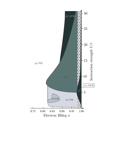
Figure 2: Schematic ground state phase diagram $(n,U/t)$ for the square lattice Hubbard model (bandwidth $8t$) for our cluster DMFT, showing a conventional paramagnetic phase (a), a paramagnetic phase with a distorted Fermi surface (b), a Slater-like antiferromagnetic phase (c), another antiferromagnetic phase (d), a pure Slater nested antiferromagnetic phase (e) and a ferromagnetic phase (f). A dashed line indicates a second order transition. The phases are characterized further in the text. Solutions for the hatched region, $0.98<n<1$, are not considered (see text).

Recall that for this model there are three important factors driving the underlying physics: the Mott transition, the nesting of the $U=0$ Fermi surface at $n=1$, and the van Hove points in the free particle dispersion at $(\pi,0)$ and $(0,\pi)$. Clearly at $n=1$ all of these factors play a rôle, but away from this point we see the three factors exerting distinct influences on the ground state physics.

V.1 Trends across the phase diagram

The solution far from half-filling ($n<0.82$), or for very small interaction strength ($U\lesssim 0.25t$), is a metallic paramagnetic phase [Fig. 2 phase (a)] with a sharply defined Fermi surface, seen as a discontinuity in $n_{{\bm{\mathrm{k}}}}$ [Fig. 7(b), dotted line]. This Fermi liquid becomes increasingly correlated as $U$ is increased; the quasiparticle residue $z$ decreases, and $n_{{\bm{\mathrm{k}}}}$ becomes more homogeneous (though maintaining a discontinuity) as weight spreads out through ${\bm{\mathrm{k}}}$-space. This reflects the local nature of the strong repulsion, $U$. Spectrally, Hubbard side bands are observed to appear, and the central quasiparticle band narrows; an example density of states is shown in Fig. 3, consistent with the three peak structure  used to understand the Mott transition. georges_1996a

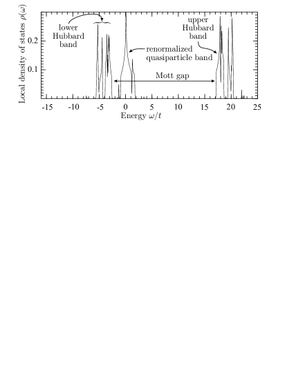
Figure 3: At $U=20t$, $n=0.8$ the ground state is paramagnetic [Fig. 2 (a)]. The smoothed local density of states for this solution is shown. The central quasiparticle peak shows a single-particle density of states, with a bandwidth $8t^{*}\sim 3t$ significantly renormalized from the original $8t$ due to correlations. Above and below the peak there are upper and lower Hubbard bands, separated by a Mott gap of size $\sim U$, and both Hubbard bands show imprints of the single-particle dispersion.

As the filling $n$ is increased nearer to 1 (half-filling), the Fermi surface in the paramagnetic state expands, and we observe a phase transition [to phase (b) of Fig. 2] where the Fermi surface breaks $x$-$y$ symmetry (see Fig. 4). It is likely that the system is exploiting the reduced Fermi velocity near the van Hove point $(0,\pi)$ to redistribute electrons in momentum space to lower the total energy—a Pomeranchuk transition. This tendency has also been seen by other authors. halboth_2000a ; hankevych_2002a ; metzner_2003a ; neumayr_2003a Note however, our cluster breaks $x$-$y$ symmetry from the outset, so this is not strictly symmetry breaking, but the degree of deviation from $x$-$y$ symmetry increases abruptly at this point.

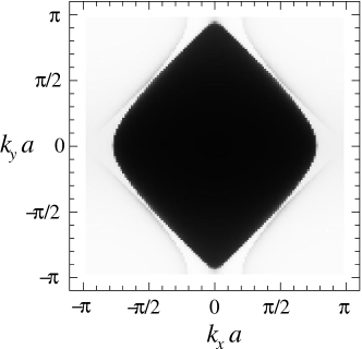
Figure 4: At $U=2t$, $n=0.90$ the ground state is paramagnetic but the Fermi surface has spontaneously distorted [Fig. 2 phase (b)]. Here the electron filling $n_{{\bm{\mathrm{k}}}}$ is shown in grayscale across the Brillouin zone: black corresponds to fully occupied states, white are completely empty states. The Fermi surface is well defined, but has undergone a Pomeranchuk transition: electrons have moved from $(\pi,0)$ to $(0,\pi)$, exploiting the flat dispersion near the van Hove point. Note the appearance of a faint “ghost” Fermi surface displaced from the original by a wavevector $(\pi/a,\pi/a)$. This is due to the effect of antiferromagnetic fluctuations.

For $U\gtrsim 6t$ and $n\gtrsim 0.8$, we find that the ground state is a spin-symmetry-broken antiferromagnetic phase [Fig. 2 phase (c)]. The Fermi surface is Pomeranchuk distorted, remaining the same shape as for the paramagnet [Fig. 2 phase (b)]. The local density of states shown in Fig. 5(a) changes little between that paramagnetic and this magnetically ordered state. Indeed, the only change is that $(n_{A\uparrow}=n_{B\downarrow})$ becomes no longer equal to $(n_{A\downarrow}=n_{B\uparrow})$. We interpret this phase as a Slater antiferromagnet because the density of states and quasiparticle dispersion is, for low $U$ at least, what one would expect from a weak spin-density wave transition on a metallic state with a gap growing like $U$ (see, for example, the mean-field theory of Schrieffer, Wen and Zhang schrieffer_1989a ). Note that here the gap in the density of states is already present in the paramagnetic state; we will refer back to this point in relation to the pseudogap physics of the cuprates.

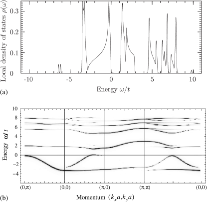
Figure 5: At $U=6t$, $n=0.88$ the ground state is an antiferromagnetic metal with a distorted Fermi surface [Fig. 2 phase (c)]. (a) The total local density of states is shown for this state (smoothed and combining up and down spins). The magnetic gap is apparent, and correlations cause further partitioning. In this region the gap size increases with increasing $U$. The densities of states for the neighboring paramagnetic solution [Fig. 2 phase (b)] are insignificantly different, although the sublattice- and spin-resolved densities of states are of course unbalanced for antiferromagnetic solutions. (b) The evolution of the electron spectral function is shown for various straight-line sections through the Brillouin zone. The plot is grayscale with darker regions representing states with higher spectral weight. As well as weakly dispersing bands at high energies, the quasiparticle dispersion can be seen for energies between $\pm 4t$. The form of the dispersion is that expected for a mean field spin-density wave state. Hence we identify the gap in the density of states as being Slater-like.

There is a second antiferromagnetic phase [Fig. 2 phase (d)] which appears when $U\gtrsim 16t$. Here the magnetic gap develops within the narrow quasiparticle peak of the density of states, which is itself well separated from two fully formed Hubbard bands in the familiar three peak structure (see Fig. 6). The momentum dependence of the narrow quasiparticle dispersion has the same structural form as that in the Slater magnetic phase above but with a greatly reduced bandwidth. This can be seen by comparing the spectral functions shown in Fig. 5(b) and Fig. 6(b) near $\omega=0$. The magnetism is thus appearing like a spin-density wave transition but now for the renormalized quasiparticles. We find that the gap reduces as $U$ is increased consistent with $\sim t^{2}/U$; thus we interpret this phase as an antiferromagnetic metal in an effective $t$-$J$ model, where $t_{\rm eff}\ll t$ and $J_{\rm eff}\sim t^{2}/U$. The neighboring paramagnetic phase (at a reduced filling of $n\lesssim 0.9$) could perhaps be described, at low energies, as a nearly-antiferromagnetic Fermi liquid.

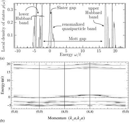
Figure 6: At $U=20t$, $n=0.9$ the ground state is also an antiferromagnetic metal with little $x-y$ symmetry breaking [Fig. 2 phase (d)]. (a) Here we show the local density of states (smoothed, up and down spins combined). The central quasiparticle peak is separated from upper and lower Hubbard bands and is heavily renormalized due to correlations. It is also gapped; this gap decreases with increasing $U$. (b) From the spectral density we identify the dispersing quasiparticle near the chemical potential. The form of the dispersion is very similar to that of Fig. 5(b), so Slater-like, but the degree of dispersion is very much reduced.

There are two other magnetic phases. First, exactly at half-filling (and extending to lower $n$ near $U\sim 5t$) there is a antiferromagnet [Fig. 2 phase (e)] of fairly pure Slater character, inevitable for a bipartite lattice. The spectrum we find is consistent with that described elsewhere in the literature, for example the separate high energy bands in Ref. dahnken_2003a, . Second, there is a small patch of low moment ferromagnetism [Fig. 2 phase (f)]; here the system is exploiting the soft Fermi surface near the van Hove points (c.f. Ref. metzner_2003a, ), and the Fermi surface for one spin species distorts more than the other.

V.2 Metal–insulator transition and the pseudogap

A key puzzle in the study of correlated electrons near the Mott transition concerns the changes in the Fermi surface as the Mott insulating state is approached. How, for example, does the large volume Fermi surface expected in a Fermi liquid obeying Luttinger’s theorem, evolve into a doped Mott insulator where it appears that the number of holes characterizes physical properties (see, for example, Ref. uemura_1989a, )? This question can be answered within the constraints of our approach: as the carrier concentration approaches half-filling, we see a large Fermi surface breaking up into hole pockets separated by regions without free carriers. In this section we will describe this process in more detail.

Well away from half-filling, we observe a distinct Fermi surface, defined by a discontinuity in $n_{\bm{\mathrm{k}}}$ [see dotted line in Fig. 7(b)], with a Luttinger volume equal to $n$. As $n\rightarrow 1$ and we approach an antiferromagnetic state, evidence of a “ghost” Fermi surface is seen: low energy electron-like excitations appear at the position of the original Fermi surface but displaced by the antiferromagnetic wavevector $(\pi,\pi)$. This can be seen as a faint line in Fig. 4. Note that the magnetic symmetry has not yet been broken.

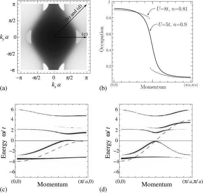
Figure 7: At $U=5t$, $n=0.9$ the ground state is paramagnetic and breaks $x$-$y$ symmetry. It also shows the breakup of the Fermi surface into hole pockets by the formation of an anisotropic gap around the Fermi surface. Fig. (a) shows $n_{{\bm{\mathrm{k}}}}$ in grayscale across the Brillouin zone (black $\leftrightarrow 1$, white $\leftrightarrow 0$). A distinct Fermi surface can be seen along some directions but not others. Fig. (b) illustrates the absence of a Fermi surface discontinuity in $n_{\mathbf{k}}$ along the line $(0,0)\rightarrow(\pi,\pi)$ (solid line). This should be compared to the form of $n_{\mathbf{k}}$ in a phase without such a gap [$(U=8t,n=0.81)$ shown by the dotted line]. The nature of the anisotropy around the Fermi surface can be seen in the electron spectral functions: (c) A grayscale plot of the spectral function (dark $\leftrightarrow$ larger weight) along the line $(0,0)\rightarrow(\pi,0)$. The chemical potential $\mu$ crosses a modified dispersion twice, creating the hole pocket—though with little weight at the second crossing point. (d) The spectral function (dark $\leftrightarrow$ larger weight) along the line $(0,0)\rightarrow(\pi,\pi)$ shows that $\mu$ falls within a gap; there is no Fermi surface along this line. The dashed line in (c) and (d) shows the non-interacting dispersion. Fig. 8 shows schematically the origin of this electronic structure.

Looking at the complete spectrum [for example in Figs 7(c) and (d)] reveals that this “ghost” Fermi surface is a manifestation of a “ghost dispersion”—the original dispersion shifted by $(\pi,\pi)$. This ghost dispersion has much less spectral weight than the original renormalized quasiparticle dispersion. Nevertheless, it hybridizes with the original dispersion to give the final electronic structure. The hybridization opens a gap in the dispersion, and the effects of the gap depend on whether the chemical potential $\mu$ falls within the gap, and how the gap evolves round the Brillouin zone. A schematic view of the origin of the electronic structure is given in Fig. 8.

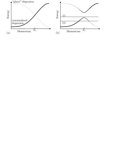
Figure 8: A schematic view of the origin of the structure of the electron spectral function in the pseudogap region [as seen within our approach in Figs 7(c) and (d)]. Darker lines carry more spectral weight. (a) Distinct fluctuations on the $A$ and $B$ sublattices result in a second dispersion of low weight (a “ghost” dispersion). This is formed by the folding of the original, possibly renormalized, dispersion in the antiferromagnetic Brillouin zone (defining $g_{m}$). (b) This hybridizes with the original dispersion and forms a gap. Along directions in momentum space where the chemical potential lies in the gap [line(i)], there is a gap in the excitation spectrum and no Fermi surface. Along directions where the chemical potential lies away from the gap it crosses the dispersion at two points [line (ii)]. A hole pocket forms with low spectral weight at the second crossing.

In the case of Fig. 4 where $U=2t$ and $n=0.90$, $\mu$ is below the gap everywhere on the Fermi surface, and crosses the new dispersion in two places; the spectral weight at the second crossing is much weaker and causes the “ghost” Fermi surface. However, if the filling is increased (raising $\mu$) or the interaction $U$ is increased, widening the hybridization gap, then the chemical potential may fall within the gap at various places around the Brillouin zone. Such an occurrence is illustrated in Fig. 7(d) for the case ($U=5t$, $n=0.90$) along the line in the Brillouin zone (0,0) to ($\pi,\pi$). With no band crossing the Fermi surface there is no discontinuity in $n_{k}$ as demonstrated in Fig. 7(b). Instead $n_{k}$ falls smoothly because of the reduced spectral weight in the “ghost” band that forms at the high momentum end of the low energy dispersion. There is a gap for single electron excitations along this direction.

This gap is a pseudogap rather than a complete gap as there are other directions where a well-defined Fermi-surface remains. Fig 7(c) shows the spectral function along the line (0,0) to ($\pi$,0). There the chemical potential crosses the spectral function dispersion in two places. The spectral weight is much weaker at the higher momentum crossing because this part of the dispersion derives mainly from the “ghost” band. These two crossings mark the edges of a hole pocket as can be seen in Fig. 7(a). The quasiparticles have developed hole-like characteristics and the Luttinger volume has changed. However, because of the evolving spectral weight in momentum space, only one side of the pocket has quasiparticles with high electron weight. These hole pockets could resemble disconnected Fermi surface arcs to experimental probes unable to resolve the small electron weight at the second dispersion crossing. A similar breakup of the Fermi surface near the Mott transition was suggested by Furakawa et al. furukawa_1998a

As $n$ increases, the hole pockets reduce in size until they become points, and subsequently vanish and the system is an insulator. This illustrates how a smooth metal-insulator transition is possible. After a pseudogap has formed, the Luttinger volume cannot be defined as usual; the active Fermi surface consists of hole pockets, and rest of the filled region of ${\bm{\mathrm{k}}}$-space is bounded by portions of the original Fermi surface where $n_{{\bm{\mathrm{k}}}}$ falls smoothly, without a step.

The features described above are reminiscent of the cuprate high-temperature superconductors in their normal state, which are believed to have a Fermi surface consisting of arc-like segments separated by pseudogap regions (see for example Refs chubukov_1997a, ; damascelli_2003a, ; yoshida_2003a, ). A picture where the dispersion relation hybridizes with a “ghost” dispersion is consistent with angle-resolved photoemission spectroscopy (ARPES) experiments (see for example Fig. 58 of Ref. damascelli_2003a, ), and also emerges from other theoretical models.chubukov_1997a

There are important differences, however, between our results and what is seen in the cuprates, most significantly in the position of the arcs and the pseudogap regions. In the cuprates the Fermi surface arcs are seen at $(\pi/2,\pi/2)$ but appear near $(0.7\pi,0)$ in our calculations, and the pseudogap occurs near $(\pi,0)$ in the cuprates but near $(\pi/2,\pi/2)$ in our calculations. However, our results are not incompatible, as restriction to a cluster with only a pair of sites severely constrains the momentum dependence of the electron self-energy. Fermi surface shapes can only be formed from the original dispersion $\epsilon_{{\bm{\mathrm{k}}}}$ in combination with the asymmetric dispersion $\epsilon_{{\bm{\mathrm{k}}}}\cos k_{x}a$ (as Eq. 17 shows). This does not admit the $d$-wave symmetry observed in the cuprates but only $s$- and $p$-wave configurations, which means for example that arcing can only happen near the van Hove points such as $(\pi,0)$. Adding more sites to the cluster would progressively optimize our approximation to the real shape, and we intend to extend our work to a four site ($2\times 2$) cluster which would permit $d$-wave symmetry, though at the price of greater numerical complexity.

VI Conclusion

We have presented the zero temperature properties of a cluster-type extension of dynamical mean-field theory, where the self-consistency equations have been solved in a very restricted basis. Our approach allows us to calculate the full phase diagram of a fully interacting system, and it can be surveyed and understood through access to complete spectral information. The basis we chose is “two-site DMFT”, whose results compare favorably with other theories and experiment; our cluster extension additionally allows a limited momentum dependence of the self-energy.

Our results provide clues to several puzzling features of the metal–insulator transition and how antiferromagnetism, proximity to van Hove points, and formation of the Mott gap compete with one another; all play a rôle in various regimes. The van Hove point causes Fermi surface distortions even at low $U$; nesting causes Slater antiferromagnetism near half-filling; and the Mott gap becomes significant at high $U$ as one might have anticipated. In addition, we see how $t$-$J$ model physics manifests itself at large $U$ via the small magnetic gap. We also see how, as the metal–insulator transition is approached, the Fermi surface evolves from a renormalized Fermi liquid obeying Luttinger’s theorem, to a pseudogap state where a gap opens on some parts of the Fermi surface breaking it up into hole pockets (with a strongly momentum-dependent spectral density).

Our work is easily extensible to more sophisticated cluster DMFT schemes or multiple bands, and we intend to study a $2\times 2$ cluster which allows tetragonal symmetry and would compare more directly with the cuprates.

We thank C. Hooley, J. Quintanilla and Q. Si for helpful discussions. We gratefully acknowledge the support of the Royal Society and the Leverhulme Trust (AJS) and EPSRC (ECC).

References

- (1) J. Hubbard. Proc. R. Soc. London Ser. A 281, 401 (1964).
- (2) W. F. Brinkman and T. M. Rice. Phys. Rev. B 2, 4302 (1970).
- (3) J. C. Slater. Phys. Rev. 82, 538 (1951).
- (4) A. Georges, et al. Rev. Mod. Phys. 68, 13 (1996).
- (5) V. I. Anisimov, et al. J. Phys. Cond. Mat. 9, 7359 (1997).
- (6) A. I. Lichtenstein and M. I. Katsnelson. Phys. Rev. B 57, 6884 (1998).
- (7) A. I. Lichtenstein, M. I. Katsnelson, and G. Kotliar. Phys. Rev. Lett. 87, 067205 (2001).
- (8) M. H. Hettler, et al. Phys. Rev. B 58, R7475 (1998).
- (9) G. Kotliar, et al. Phys. Rev. Lett. 87, 186401 (2001).
- (10) A. I. Lichtenstein and M. I. Katsnelson. Phys. Rev. B 62, R9283 (2000).
- (11) M. Potthoff. Phys. Rev. B 64, 165114 (2001).
- (12) M. Caffarel and W. Krauth. Phys. Rev. Lett. 72, 1545 (1994).
- (13) C. J. Halboth and W. Metzner. Phys. Rev. Lett. 85, 5162 (2000).
- (14) V. Hankevych, I. Grote, and F. Wegner. Phys. Rev. B 66, 094516 (2002).
- (15) W. Metzner, D. Rohe, and S. Andergassen. Phys. Rev. Lett. 91, 066402 (2003).
- (16) A. Neumayr and W. Metzner. Phys. Rev. B 67, 035112 (2003).
- (17) M. Jarrell. Phys. Rev. Lett. 69, 168 (1992).
- (18) A. Koga, et al. eprint cond-mat/0401223.
- (19) T. A. Maier, T. Pruschke, and M. Jarrell. Phys. Rev. B 66, 075102 (2002).
- (20) C. Huscroft, et al. Phys. Rev. Lett. 86, 139 (2001).
- (21) C. Dahnken, et al. eprint cond-mat/0309407.
- (22) O. Parcollet, G. Biroli, and G. Kotliar. eprint cond-mat/0308577.
- (23) G. Biroli, O. Parcollet, and G. Kotliar. eprint cond-mat/0307587.
- (24) W. H. Press, et al. Numerical Recipes in C (Cambridge University Press, 1992).
- (25) A. L. Fetter and J. D. Walecka. Quantum Theory of Many-Particle Systems (McGraw-Hill, 1971). Eqn (9.36).
- (26) J. R. Schrieffer, X. G. Wen, and S. C. Zhang. Phys. Rev. B 39, 11663 (1989).
- (27) Y. J. Uemura, et al. Phys. Rev. Lett. 62, 2317 (1989).
- (28) N. Furukawa, T. M. Rice, and M. Salmhofer. Phys. Rev. Lett. 81, 3195 (1998).
- (29) A. V. Chubukov and D. K. Morr. Phys. Reports 288, 355 (1997).
- (30) A. Damascelli, Z. Hussain, and Z.-X. Shen. Rev. Mod. Phys. 75, 473 (2003).
- (31) T. Yoshida, et al. Phys. Rev. Lett. 91, 027001 (2003).