Exact Ground-State Energies of the Random-Field Ising Chain and Ladder

Abstract

We derive the exact ground-state energy of the one-dimensional Ising model in random fields taking values $h$, 0 and $-h$ with general probabilities. The random-field Ising model on a ladder is also analyzed by showing its equivalence to the random-field Ising chain with field values $\pm h$ and 0 for $h<J$. The zero-temperature transger matrix is used to obtain the results.

1 Introduction

The one-dimensional random-field Ising model is one of the simplest examples of systems with quenched disorder. In the long history of its intensive studies, a number of results have been published which give exact solutions in the ground state. Derrida et al[1] first derived the exact expression of the ground-state energy by a recursive calculation of the zero-temperature transfer matrix. They also obtained the exact ground-state energies of the one-dimensional random bond Ising model in a uniform field, the random bond Ising ladder and the $3\times 3$ square lattice system. Farhi and Gutmann[2] obtained the exact spin-spin correlation function of the one-dimensional random-field Ising model. Their approach is based on the ground-state spin configuration associated with the general rule that dictates which regions of the random field configurations necessarily determine the spin configuration. This method is related to another method which calculates exactly the energy and the entropy of the random-bond Ising model at zero temperature[3]. The application of the method proposed by Derrida et al to error-correcting codes was performed by Dress et al[4]. They investigated a simple error-correcting code through the zero-temperature properties of a related spin model. Further generalization of the method proposed by Dress et al was carried out by Kadowaki et al[5]. They calculated exactly the ground-state energies of the $\pm J$ random bond model and the site-random model on strips of various widths. Studies of the effects of continuous random fields in the ground state related to hysteresis are also found in Refs. [S96][S00][DDMZ02].

In the present paper, we derive the exact ground-state energy of the one-dimensional Ising model in random fields consisting three possible values $\pm h$ and 0 using a generalization of the methods in Refs. [DAL95] and [KNN96]. The solution is piecewise linear as a function of the random-field strength, a property shared with the case of random fields $\pm h$. We also find that the one-dimensional Ising model in random fields $\pm h$ and 0 is equivalent to the Ising spin ladder in random fields $\pm h$ as long as $h$ is smaller than the exchange interaction $J$. This observation leads to the exact expression of the ground-state energy of the ladder under random field, which represents the first exact solution for the random-field Ising ladder.

The present paper is composed of seven sections. In §2, we introduce our model and explain the formulation of our method based on the zero-temperature transfer matrix. An important feature of the ground state of the one-dimensional Ising model in random fields is explained in §3. The explicit evaluation of the probability distribution of a relevant quantity and the exact ground-state energy are shown in §4 and §5. A useful property for diagonalization of the transition matrix is also given. In §6, we consider the Ising ladder in $\pm h$ random fields and show that this model is equivalent to the one-dimensional Ising model with three possible random fields $\pm h$ and 0 if $h<J$. The exact ground-state energy of the ladder model is derived using the result for the one-dimensional case. Finally in §7, results are discussed.

2 Ising spin chain in the general random field

2.1 Model

Our problem is defined by the Hamiltonian

$$H=-J\sum_{n=1}^{N}S_{n-1}S_{n}-\sum_{n=1}^{N}h_{n}S_{n},$$ (1)

where $J$ is the ferromagnetic coupling constant, $S_{n}(=\pm 1)$ is the Ising spin variable and $N+1$ is the number of spins. We use an open boundary condition. The random field at site $n$ consists of three possible values with probabilities

$$P(h_{n})=\left\{\begin{array}[]{ccl}p&\textrm{for}&h_{n}=+h\\ q&\textrm{for}&h_{n}=0\\ r&\textrm{for}&h_{n}=-h\\ \end{array}\right.,\hskip 28.45274ptp+q+r=1.$$ (5)

Almost all of the previous studies concentrated on the case $q=0$. The partition function of this model with spin $S_{N}$ on the right edge fixed is

$$Z_{N}(S_{N})=\sum_{S_{0}}\sum_{S_{1}}\cdots\sum_{S_{N-1}}\prod_{n=1}^{N}\exp\{\beta(JS_{n-1}S_{n}+h_{n}S_{n})\},$$ (6)

where $\beta$ is the inverse temperature. We can construct the partition function $Z_{N+1}(S_{N+1})$ recursively as

$$Z_{N+1}(S_{N+1})=\sum_{S_{N}}Z_{N}(S_{N})\exp(\beta(JS_{N}S_{N+1}+h_{N+1}S_{N+1})).$$ (7)

To simplify this expression, we rewrite (7) by using a $2\times 2$ matrix. Let us introduce the notation $Z_{N}^{\pm}\equiv Z_{N}(S_{N}=\pm 1)$. The recursion relation (7) can then be written as

$$\left[\begin{array}[]{c}Z_{N+1}^{+}\\ Z_{N+1}^{-}\\ \end{array}\right]=T_{N+1}\left[\begin{array}[]{c}Z_{N}^{+}\\ Z_{N}^{-}\\ \end{array}\right],$$ (12)

where $T_{N}$ is the transfer matrix

$$T_{N}=\left[\begin{array}[]{cc}z^{J+h_{N}}&z^{-J+h_{N}}\\ z^{-J-h_{N}}&z^{J-h_{N}}\\ \end{array}\right],$$ (15)

with $z={\rm e}^{\beta}$.

2.2 Recursion relations in the zero-temperature limit

In the limit of very low temperatures, the partition function $Z_{N}(S_{N})$ can be expressed in terms of the ground-state energy as

$$Z_{N}(S_{N})\simeq\exp(\beta x_{N}(S_{N}))=z^{x_{N}(S_{N})},$$ (16)

where $x_{N}(S_{N})$ is the ground-state energy with the edge spin state $S_{N}$. If we use the expressions $x_{N}(+1)=x_{N}$ and $x_{N}(-1)=x_{N}+2a_{N}$, we have in the zero temperature limit

$$\left[\begin{array}[]{c}Z_{n}^{+}\\ Z_{n}^{-}\end{array}\right]\simeq\left[\begin{array}[]{l}z^{x_{n}}\\ z^{x_{n}+2a_{n}}\end{array}\right].$$ (21)

Substituting eqn. (21) into eqn. (12), we obtain the following recursion relations,

$$x_{n+1} = x_{n}+J+h_{n+1}+2\,{\rm max}(0,a_{n}-J)$$ (22)

$$a_{n+1} = f(a_{n})-h_{n+1},$$ (23)

where $f(a_{n})$ is a piecewise linear function defined as

$$f(a_{n})=\left\{\begin{array}[]{ccl}+J&\textrm{for}&a_{n}>J\\ a_{n}&\textrm{for}&-J<a_{n}<J\\ -J&\textrm{for}&a_{n}<-J\end{array}\right..$$ (27)

As shown below, from the recursion relation (22), the average of the ground-state energy over random fields reduces to the average of ${\rm max}(0,a_{n}-J)$ over the distribution of the energy difference $a_{n}$. We note that recursion relations (22) and (23) always hold for any types of random fields, not necessarily of eqn. (5).

2.3 Ground-state energy

Using the recursion relation (22), we can express the ground-state energy per spin as

$$E_{\rm GS} = \lim_{N\rightarrow\infty}\frac{1}{N}\left(-\frac{1}{\beta}\log Z_{N}\right)$$ (28)

$$= -\lim_{N\rightarrow\infty}\frac{1}{N}\left\{x_{N}+{\rm max}(0,2a_{N})\right\}$$

$$= -\lim_{N\rightarrow\infty}\frac{1}{N}\left\{\sum_{n=0}^{N-1}(x_{n+1}-x_{n})+x_{0}+{\rm max}(0,2a_{N})\right\}$$

$$= -J-(p-r)h-2\left\langle\left\langle{\rm max}(0,a-J)\right\rangle\right\rangle,$$

where $a$ is the energy difference in the limit $N\rightarrow\infty$ and the double brackets $\langle\langle\cdots\rangle\rangle$ mean the average over the probability distribution of the energy difference $P(a)$. To obtain the last line of eqn. (28), we have invoked the self-averaging property of the energy.

According to eqn. (28), we have to derive the probability distribution of the energy difference $P(a)$. The derivation of $P(a)$ is given in §4. Before going into the detailed evaluation of $P(a)$, we explain another important feature of the ground state of the present model.

3 Spin configurations in the ground state

In this section, we consider the spin configuration in the ground state by evaluating the energy for specific configuration of random fields. From this argument, we derive an important property of the Ising model in random fields.

We first consider the case $q=0$ $(h_{n}=\pm h)$. If the random-field strength $h$ is larger than $2J$, we can easily obtain the ground-state spin configuration because all spins are forced to be parallel to the random field. However, for $h<2J$, the ground state has non-trivial spin configurations as discussed now.

First let us consider the following random-field configuration which consists of the field $+h$ at all but a single site,

$$\cdots+++++-+++++\cdots,$$ (29)

where the symbol $+$ represents the field $+h$ and $-$ refers to the field $-h$. All spins are parallel to the random field when $h$ is larger than $2J$. However, if $h<2J$, all spins are up ($S_{n}=1$). To see this, we evaluate the energy difference between the two spin configurations,

$$E_{1}=+2J-h+E_{+}$$ (30)

$$E_{2}=-2J+h+E_{+}$$ (31)

$$\Delta E=E_{2}-E_{1}=-4J+2h,$$ (32)

where $E_{1}$ is the energy for all spins parallel to the field, $E_{2}$ represents the energy of all-up spin state and $E_{+}$ means the energy resulting from all sites except for the location of field $-h$. According to eqn. (32), for $h>2J$, the ground-state energy is $E_{1}$, and it is $E_{2}$ otherwise. We note that the ground-state energy is doubly degenerate at $h=2J$.

Next we consider the following configuration of the random field which consists of the field $+h$ at all sites except for two adjacent sites

$$\cdots+++++--+++++\cdots.$$ (33)

Similar arguments as above lead to the conclusion that all spins point parallel to the random field if $h>J$, and all spins are up if $h<J$. The ground-state energy is degenerate at $h=J$.

We can apply these arguments to the general case with $k$ pieces of successive random fields taking the value $-h$,

$$\cdots+++++\underbrace{---\cdots---}_{k}++++\cdots,$$ (34)

for which

$$E_{1}=+2J-kh+E_{+}$$ (35)

$$E_{2}=-2J+kh+E_{+}$$ (36)

$$\Delta E=E_{2}-E_{1}=-4J+2kh,$$ (37)

where the definitions of $E_{1}$, $E_{2}$ and $E_{+}$ remain the same as in the case of eqn. (29). The ground-state energy changes from $E_{1}$ to $E_{2}$ at $h=2J/k$ and these two energies are degenerate at $h=2J/k$. Consequently, the ground state of the one-dimensional Ising model in the random field changes at the random-field strength $h=2J/k$, where $k$ is an integer.

To understand it, we consider the following configuration of the random field,

$$\cdots+++\underbrace{-}_{A}+++\cdots+++\underbrace{--}_{B}+++\cdots+++\underbrace{---}_{C}+++\cdots,$$ (38)

where $A$, $B$ and $C$ are the clusters of fields pointing to the $-$ direction with length one, two and three. There are several clusters of fields taking the value $-h$ in the sea of fields taking the value $+h$. In the case of $h>2J$, all spins are parallel to random fields. When $h$ decreases and satisfies $h<2J$, the spin at the cluster with length one (that is, the part $A$ in (38)) flips its direction from down to up. Next, spins at the cluster of length two (the part $B$ in (38)) flip their direction from down to up when $h$ decreases and satisfies $h<J$. The ground-state proceeds with this change, and spins in the cluster with length $k$ flip their direction from $-h$ to $+h$ when the random-field strength reaches $h=2J/k$. The ground-state spin configurations are invariant in the range

$$\frac{2}{k+1}J<h<\frac{2}{k}J.$$ (39)

Within this range the ground-state energy is a linear function of the random-field strength $h$. The same discussion as above holds if we include the possibility of random-field value of $0$.

4 Probability distribution

For explicit evaluation of the ground-state energy, we should find the probability distribution of the energy difference $P(a)$ according to eqn. (23). In this section, we calculate this probability distribution $P(a)$ by the recursion relation (23) following the idea of Refs. [DAL95] and [KNN96].

4.1 From recursion relation to transition matrix

Let us see how the $a$’s are generated stochastically by the recursion relation (23). For example, we first consider the simplest case of the random field strength $h>2J$. We start the recursion relation from the initial condition $a_{0}=0$ and obtain $a_{1}=-h$ for $h_{1}=h$, $a_{1}=0$ for $h_{1}=0$ and $a_{1}=h$ for $h_{1}=-h$. The next value of $a_{n}$ is

$$\begin{array}[]{lcll}a_{2}=-J-h&\textrm{for}&a_{1}=-h,&h_{2}=h\\ a_{2}=-J&\textrm{for}&a_{1}=-h&h_{2}=0\\ a_{2}=-J+h&\textrm{for}&a_{1}=-h,&h_{2}=-h\\ a_{2}=-h&\textrm{for}&a_{1}=0,&h_{2}=h\\ a_{2}=0&\textrm{for}&a_{1}=0,&h_{2}=0\\ a_{2}=+h&\textrm{for}&a_{1}=0,&h_{2}=-h\\ a_{2}=J-h&\textrm{for}&a_{1}=h,&h_{2}=h\\ a_{2}=J&\textrm{for}&a_{1}=h,&h_{2}=0\\ a_{2}=J+h&\textrm{for}&a_{1}=h,&h_{2}=-h\end{array}.$$ (49)

No other values emerge for $a_{n}$ ($n\geq 3$) as can be verified by repeating this procedure. Consequently, we can regard the recursion relation (23) as a stochastic process with the transition matrix

$$S_{0}=\left[\begin{array}[]{ccc}P+Q&P&P\\ 0&Q&0\\ R&R&Q+R\\ \end{array}\right],$$ (53)

where

$$P=\left[\begin{array}[]{ccc}p&0&0\\ q&0&0\\ r&0&0\\ \end{array}\right],\hskip 14.22636ptQ=\left[\begin{array}[]{ccc}0&p&0\\ 0&q&0\\ 0&r&0\\ \end{array}\right],\hskip 14.22636ptR=\left[\begin{array}[]{ccc}0&0&p\\ 0&0&q\\ 0&0&r\\ \end{array}\right].$$ (63)

The row and column of matrix (53) correspond to the following vector of the energy differences

$$\left[\begin{array}[]{c}-J-h\\ -J\\ -J+h\\ -h\\ 0\\ +h\\ J-h\\ J\\ J+h\\ \end{array}\right].$$ (73)

For example, the $(1,1)$-component of matrix (53) means that the energy difference $-J-h$ remains unchanged with probability $p$. The stationary distribution $P(a)$ is given by the eigenvector of this transition matrix with the eigenvalue 1, and the result is

$$\left[\begin{array}[]{c}P(-J-h)\\ P(-J)\\ P(-J+h)\\ P(-h)\\ P(0)\\ P(+h)\\ P(J-h)\\ P(J)\\ P(J+h)\\ \end{array}\right]=\left[\begin{array}[]{c}\frac{p^{2}}{p+r}\\ \frac{pq}{p+r}\\ \frac{pr}{p+r}\\ 0\\ 0\\ 0\\ \frac{pr}{p+r}\\ \frac{qr}{p+r}\\ \frac{r^{2}}{p+r}\\ \end{array}\right].$$ (92)

This result holds in the region $h>2J$, the case of $k=0$ in eqn. (39). The ground state is invariant in the region of $h>2J$. This means that the stationary state of the range $h>2J$ is always described by the transition matrix $S_{0}$ and the probability distribution $P(a)$ remains invariant throughout the range $h>2J$. A similar property holds in other ranges specified by eqn. (39).

Applying the same argument to the case of $k\neq 0$, we obtain the following $3(2k+3)\times 3(2k+3)$ transition matrix

$$S_{k}=\left[\begin{array}[]{cccccc|c|cccccc}P+Q&P&0&\cdots&0&0&P&P&&&&&\\ R&Q&P&\cdots&0&0&0&&&&&&\\ 0&R&Q&&0&0&0&&&&\text{\huge{0}}&&\\ \vdots&\vdots&&\ddots&\vdots&\vdots&\vdots&&&&&&\\ 0&0&0&\cdots&Q&P&0&&&&&&\\ 0&0&0&\cdots&R&Q&0&&&&&&\\ \hline\cr 0&0&0&\cdots&0&0&Q&0&0&\cdots&0&0&0\\ \hline\cr&&&&&&0&Q&P&\cdots&0&0&0\\ &&&&&&0&R&Q&\cdots&0&0&0\\ &&&&&&\vdots&\vdots&\vdots&\ddots&&\vdots&\vdots\\ &&\text{\huge{0}}&&&&0&0&0&\cdots&Q&P&0\\ &&&&&&0&0&0&\cdots&R&Q&P\\ &&&&&R&R&0&0&\cdots&0&R&Q+R\\ \end{array}\right].$$ (106)

The row and column of the matrix $S_{k}$ correspond to the following vector of the energy differences,

$$\left[\begin{array}[]{c}-J-h\\ -J\\ -J+h\\ -J+h-h\\ -J+h\\ -J+h+h\\ \vdots\\ -J+kh-h\\ -J+kh\\ -J+kh+h\\ -h\\ 0\\ +h\\ J-kh-h\\ J-kh\\ J-kh+h\\ \vdots\\ J-h-h\\ J-h\\ J-h+h\\ J-h\\ J\\ J+h\\ \end{array}\right].$$ (130)

Evaluation of the eigenvector of the matrix $S_{k}$ is not simple because this matrix includes $3\times 3$ matrices $P$, $Q$ and $R$. This difficulty can be resolved by the decomposition of the eigenvector into a direct product. The details are explained in Appendix. We only show the result here. The eigenvector of the matrix $S_{k}$ with eigenvalue 1 is given as

$${\textnormal{$v$}}={\textnormal{$v_{0}$}}\otimes\left(\begin{array}[]{c}p\\ q\\ r\\ \end{array}\right),$$ (134)

where $v_{0}$ is the eigenvector of the $(2k+3)\times(2k+3)$ matrix

$$S_{k}=\left[\begin{array}[]{cccccc|c|cccccc}p+q&p&0&\cdots&0&0&p&p&&&&&\\ r&q&p&\cdots&0&0&0&&&&&&\\ 0&r&q&&0&0&0&&&&\text{\huge{0}}&&\\ \vdots&\vdots&&\ddots&\vdots&\vdots&\vdots&&&&&&\\ 0&0&0&\cdots&q&p&0&&&&&&\\ 0&0&0&\cdots&r&q&0&&&&&&\\ \hline\cr 0&0&0&\cdots&0&0&q&0&0&\cdots&0&0&0\\ \hline\cr&&&&&&0&q&p&\cdots&0&0&0\\ &&&&&&0&r&q&\cdots&0&0&0\\ &&&&&&\vdots&\vdots&\vdots&\ddots&&\vdots&\vdots\\ &&\text{\huge{0}}&&&&0&0&0&\cdots&q&p&0\\ &&&&&&0&0&0&\cdots&r&q&p\\ &&&&&r&r&0&0&\cdots&0&r&q+r\\ \end{array}\right].$$ (148)

with eigenvalue 1.

4.2 Probability distribution

Diagonalizing the transition matrix (106), we obtain the probability of the energy difference $P(a)$. For this purpose, the relation (134) is useful. We define the following eigenvector of the matrix (148),

$${\textnormal{$v_{0}$}}^{T}=(D_{1},D_{2},\cdots,D_{k},D_{k+1},0,D_{\overline{k+1}},D_{\overline{k}},\cdots,D_{\overline{2}},D_{\overline{1}}).$$ (149)

Using this expression of the vector $v_{0}$, we obtain the following results

$$D_{m}=\frac{\displaystyle\sum_{l=m}^{k+1}\left(\frac{r}{p}\right)^{l-1}}{\displaystyle\sum_{l=1}^{k+1}\left(\frac{r}{p}\right)^{l-1}\sum_{l=1}^{k+2}\left(\frac{r}{p}\right)^{l-1}},\hskip 14.22636ptD_{\overline{m}}=\frac{\displaystyle\sum_{l=m}^{k+1}\left(\frac{p}{r}\right)^{l-1}}{\displaystyle\sum_{l=1}^{k+1}\left(\frac{p}{r}\right)^{l-1}\sum_{l=1}^{k+2}\left(\frac{p}{r}\right)^{l-1}},$$ (150)

where integer $m$ runs from 1 to $k+1$ and is specified by the range of the random-field strength as in eqn. (39). The probability distribution of the energy difference $P(a)$ corresponds to the eigenvector $v$ as

$$\left[\begin{array}[]{c}P(-J-h)\\ P(-J)\\ P(-J+h)\\ P(-J+h-h)\\ P(-J+h)\\ P(-J+h+h)\\ \vdots\\ P(-J+kh-h)\\ P(-J+kh)\\ P(-J+kh+h)\\ P(-h)\\ P(0)\\ P(+h)\\ P(J-kh-h)\\ P(J-kh)\\ P(J-kh+h)\\ \vdots\\ P(J-h-h)\\ P(J-h)\\ P(J-h+h)\\ P(J-h)\\ P(J)\\ P(J+h)\\ \end{array}\right]=\left[\begin{array}[]{c}pD_{1}\\ qD_{1}\\ rD_{1}\\ pD_{2}\\ qD_{2}\\ rD_{2}\\ \vdots\\ pD_{k+1}\\ qD_{k+1}\\ rD_{k+1}\\ 0\\ 0\\ 0\\ pD_{\overline{k+1}}\\ qD_{\overline{k+1}}\\ rD_{\overline{k+1}}\\ \vdots\\ pD_{\overline{2}}\\ qD_{\overline{2}}\\ rD_{\overline{2}}\\ pD_{\overline{1}}\\ qD_{\overline{1}}\\ rD_{\overline{1}}\end{array}\right].$$ (197)

This is the final expression of the probability distribution of the energy difference $P(a)$.

5 Exact energy

Finally, we obtain the ground-state energy for $2J/(k+1)<h<2J/k$ using eqn. (197) as

$$E_{\rm GS} = \left\{-1+\frac{4(pr)^{k+1}(p-r)^{2}}{A(k+1)A(k+2)}\right\}J$$ (198)

$$-\left\{1-q+\frac{2(pr)^{k+1}(k+1)(p-r)^{2}}{A(k+1)A(k+2)}-\frac{2A(k+1)pr}{A(k+2)}\right\}h,$$

where $A(k)$ is

$$A(k)=p^{k}-r^{k}.$$ (199)

In Fig. 1, we plot the ground-state energy eqn. (198) as a function of the random-field strength $h$ for several probabilities.

Figure 1: The ground-state energy of the random-field Ising chain with $h_{n}=\pm h$ and 0.

6 Ising spin ladder in bimodal random fields

Next, we consider the Ising spin ladder in bimodal random fields $\pm h$. For this model, we can prove its equivalence to the one-dimensional model discussed in the previous sections when $h<J$. The exact ground-state energy of the ladder model is calculated exactly using the result in eqn. (198).

6.1 Spin configuration for $h<J$

It is possible to show that for the random-field strength $h$ smaller than $J$, the Ising spin ladder in the bimodal random field is equivalent to the one-dimensional Ising model in random fields $\pm h$ and 0.

Let us consider the specific random-field configuration which consists of the fields being $-h$ in the first chain and $+h$ in the second chain (Fig. 2). For this random-field configuration, there are two possible ground states. One consists of all spins being up (or down due to the symmetry), and the other is all spins being parallel to the field. We introduce the notation $E_{\rm allup}$ for the energy of the first ground state and $E_{\rm fields}$ for the energy of the second ground state. The energies $E_{\rm allup}$ and $E_{\rm fields}$ are

$$E_{\rm allup} = -2(n-1)J-nh+n(h-J)$$ (200)

$$E_{\rm fields} = -2(n-1)J-nh+n(J-h),$$ (201)

where $n$ is the number of the rungs. If the random-field strength $h$ is smaller than $J$, the ground-state energy becomes $E_{\rm allup}$, and the ground state is all spins being up or down with equal probability. Let us consider a general random-field configuration as shown in Fig. 3. All spins in the parts $A$ and $B$ should be up or down from the above discussion. The spins in the left-most rung should be up because the fields on this rung are $+h$, and the spins between the parts $A$ and $B$ are also up for the same reason as the left-most rung. Accordingly, the spins in the part $A$ should be up. The spins in the right-most rung should be down for the fields on this rung being down, and there are two degenerate states between all spins in the part $B$ being up and down. The same argument as above holds for any other random-field configurations. For any case, the spins in the same rung are parallel. Consequently, we conclude that for $h<J$, two spins on the same rung in the ladder model always point to the same direction. Therefore, by identifying spins on the same rung as a spin taking the values $\pm 1$, we obtain the effective coupling constant $2J$ and the three kinds of effective fields $\{+2h,0,-2h\}$. This means that the ladder model in the bimodal random field is equivalent to the Ising chain in random fields $\pm h$ and 0.

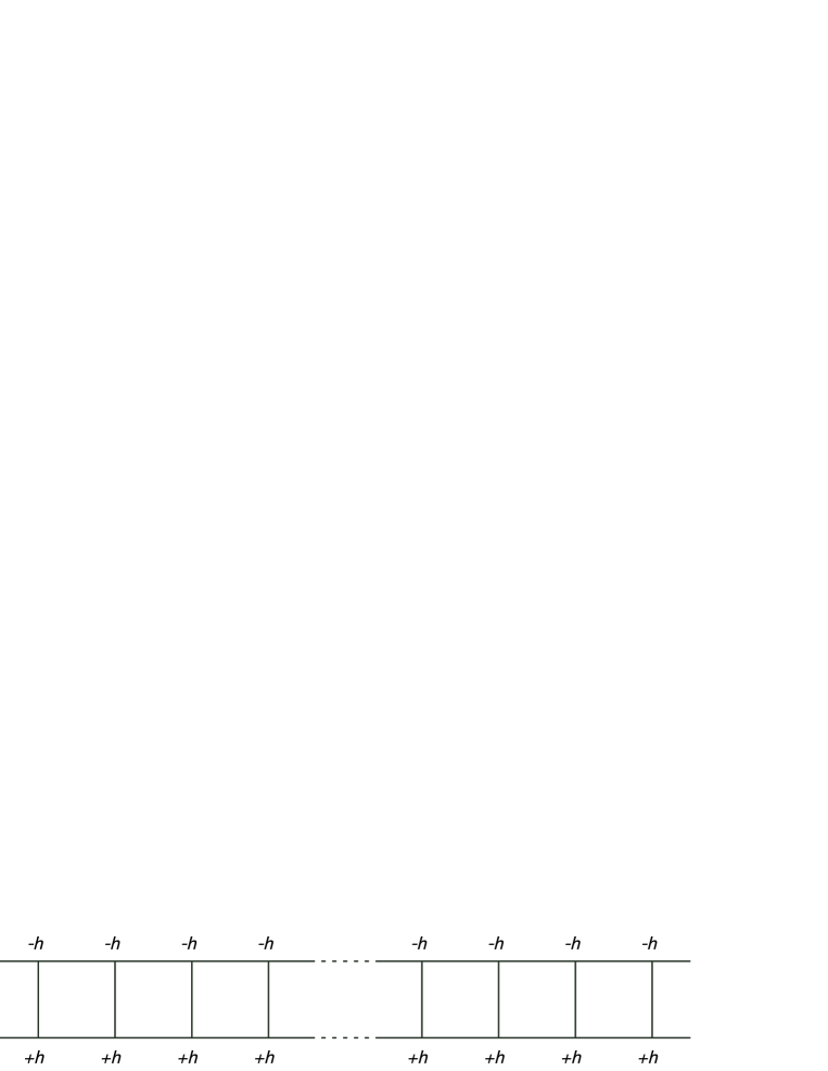
Figure 2: The configuration of fields being $-h$ in the first chain and $+h$ in the second chain.

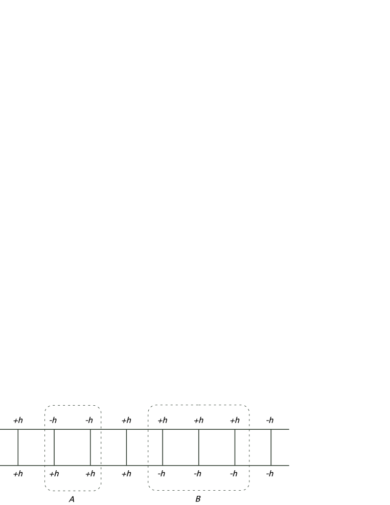
Figure 3: The general random-field configuration. The spins in parts $A$ and $B$ should be parallel for $h<J$.

6.2 Exact energy

From above argument, the exact ground-state energy of the ladder model can be obtained from the result in eqn. (198). The corresponding probabilities of the random field are

$$\begin{array}[]{lcc}p=x^{2}&{\rm for}&+h\\ q=2x(1-x)&{\rm for}&0\\ r=(1-x)^{2}&{\rm for}&-h\\ \end{array},$$ (205)

where $x$ means the probability of the random field being $+h$ for the ladder model. We also replace the random field strength and the coupling constant of the one-dimensional model with $J\rightarrow 2J$ and $h\rightarrow 2h$. We need an additional term $J$ which is caused by spins on the same rung pointing to the same direction, and divide the result by 2 because the number of spins in ladder model is twice as many as the one-dimensional model. The final expression is

$$E_{\rm GS} = \left\{-\frac{3}{2}+\frac{4(pr)^{k+1}(p-r)^{2}}{A(k+1)A(k+2)}\right\}J$$ (206)

$$-\left\{1-q+\frac{2(pr)^{k+1}(k+1)(p-r)^{2}}{A(k+1)A(k+2)}-\frac{2A(k+1)pr}{A(k+2)}\right\}h,$$

where $A(k)$ is

$$A(k)=p^{k}-r^{k}.$$ (207)

7 Discussion

In the present paper, we have derived the exact ground-state energy of the random-field Ising chain with field values $\pm h$ and 0 using the zero-temperature transfer matrix method in Refs. [DAL95] and [KNN96]. We have also obtained the exact ground-state energy of the Ising ladder in bimodal random fields for $h<J$. As far as we know this is the first example in which an exact solution has been derived for ladder model in random fields. The present techniques is a step toward a solution of random-field Ising models on strips with wider widths, eventually reaching the two-dimensional model.

We give a few comments on some aspects other than the ground-state energy. First, it should be possible to derive the exact solution for other physical quantities than the ground-state energy, such as the entropy and magnetization, using the methods in Refs. [DVP78] and [R93]. Investigations in this direction are under way.

For the Ising ladder in bimodal random fields, the evaluation of the transition matrix is not straightforward for $h>J$ since we cannot map the problem to the one-dimensional model. This difficulty is caused by the complicated structure of the recursion relation of the ladder model. In fact, we find four kinds of recursion relations to evaluate the probability distribution of the energy differences. It is not easy to construct the general form of the transition matrix from these recursion relations. This is nevertheless an important and challenging task because of the eventual target of the two-dimensional model as mentioned above.

Appendix A Decomposition of eigenvectors into a direct product

The matrix (106) is not simple to diagonalize because it is composed of the $3\times 3$ matrices $P$, $Q$ and $R$. To diagonalize this $3(2k+3)\times 2(2k+3)$ matrix, we use the decomposition of the eigenvector into a direct product. We define the following vector $w$,

$${\textnormal{$w$}}=\left(\begin{array}[]{c}p\\ q\\ r\\ \end{array}\right).$$ (211)

This vector satisfies the following relations

$$P{\textnormal{$w$}}=p{\textnormal{$w$}},\hskip 14.22636ptQ{\textnormal{$w$}}=q{\textnormal{$w$}}.$$ (212)

Using eqn. (212), we can decompose the eigenvector $v$ of the matrix $S_{k}$ into a direct product of vectors $v_{0}$ and $w$ as

$${\textnormal{$v$}}={\textnormal{$v$}}_{0}\otimes{\textnormal{$w$}},$$ (213)

where $v_{0}$ is the eigenvector of matrix $\tilde{S}_{k}$ in eqn. (148) with eigenvalue 1. To prove eqn. (213), we show that the vector ${\textnormal{$v_{0}$}}\otimes{\textnormal{$w$}}$ satisfies the equation for the eigenvector of the matrix $S_{k}$ with eigenvalue 1 as

$$S_{k}{\textnormal{$v$}}=S_{k}({\textnormal{$v$}}_{0}\otimes{\textnormal{$w$}})=(\tilde{S}_{k}{\textnormal{$v$}}_{0})\otimes{\textnormal{$w$}}={\textnormal{$v$}}_{0}\otimes{\textnormal{$w$}}={\textnormal{$v$}}.$$ (214)

Thus eqn. (213) holds. Accordingly, it is useful for the evaluation of the probability distribution that we calculate the eigenvector of the matrix $\tilde{S}_{k}$ with eigenvalue 1 instead of the eigenvector of the matrix $S_{k}$ with eigenvalue 1.

References

- [1] B. Derrida, J. Vannimenus and Y. Pomeau: J. Phys. C 11 (1978) 4749.
- [2] E. Farhi and S. Gutmann: Phys. Rev. B 48 (1993) 9508.
- [3] A. Vilenkin: Phys. Rev. B 18 (1978) 1474.
- [4] C. Dress, E. Amic and J. M. Luck: J. Phys. A: Math. Gen. 28 (1995) 135.
- [5] T. Kadowaki,Y. Nonomura and H. Nishimori: J. Phys. Soc. Jpn. 65 (1996) 1609.
- [6] P. Shukla: Physica A 233 (1996) 235.
- [7] P. Shukla: Phys. Rev. E 62 (2000) 4725.
- [8] L. Dante, G. Durin, A. Magni and S. Zapperi: Phys. Rev. B 65 (2002) 144441.
- [9] P. Rujan: Phys. Rev. Lett 70 (1993) 2968.