Noise-induced reentrant transition of the stochastic Duffing oscillator

Abstract

We derive the exact bifurcation diagram of the Duffing oscillator with parametric noise thanks to the analytical study of the associated Lyapunov exponent. When the fixed point is unstable for the underlying deterministic dynamics, we show that the system undergoes a noise-induced reentrant transition in a given range of parameters. The fixed point is stabilised when the amplitude of the noise belongs to a well-defined interval. Noisy oscillations are found outside that range, i.e., for both weaker and stronger noise.

In a classical calculation, Kapitza (1951) has shown that the unstable upright position of an inverted pendulum can be stabilised if its suspension axis undergoes sinusoidal vibrations of high enough frequency landau . More generally, stabilisation can also be obtained with random forcing graham ; luecke ; landa . In both cases, analytical derivations of the stability limit are based on perturbative approaches, i.e., in the limit of small forcing or noise amplitudes.

In a recent work kirphil , we studied the Duffing oscillator with parametric white noise when the fixed point of the underlying deterministic equation is stable: a purely noise-induced transition lefever occurs when stochastic forcing is strong enough compared to dissipation so as to ‘lift’ the system away from the absolute minimum of the potential well. We showed, using a factorisation argument, that the noise-induced transition occurs precisely when the Lyapunov exponent of the linearised stochastic equation changes sign. An analytical calculation of the Lyapunov exponent allowed us to deduce for all parameter values the bifurcation diagram, that was previously known only in the small noise (perturbative) limit. The relation between stochastic transitions in a nonlinear Langevin equation and the sign of the Lyapunov exponent is in fact mathematically rigorous and has been proved under fairly general conditions arnold . In kirphil , we also made the following striking observation: close to the bifurcation, the averaged observables of the oscillator (energy, amplitude square and velocity square), as well as all their non-zero higher-order moments, scale linearly with the distance from the threshold. This multifractal behaviour may provide a generic criterion to distinguish noise-induced transitions from ordinary deterministic bifurcations.

In the present work, we reformulate the stochastic stabilisation of an unstable fixed point of the underlying deterministic system within the framework of noise-induced transitions. We extend the analysis of kirphil and derive the full phase diagram of an inverted Duffing oscillator. We show in particular that a reentrant transition occurs in this zero-dimensional system. (Reentrant transitions induced by noise have been studied in the more complex setting of spatially extended systems vandenbroeck ). Moreover, the inverted Duffing oscillator also exhibits a multifractal behaviour close to the transition point.

The dissipative stochastic system considered here is defined by the equation:

$$\frac{\mathrm{d}^{2}x}{\mathrm{d}t^{2}}+\gamma\frac{\mathrm{d}x}{\mathrm{d}t}+\sqrt{{\mathcal{D}}}\xi(t)x=-\frac{\partial{\mathcal{U}}}{\partial x}\,,$$ (1)

where $x(t)$ is the position of the oscillator at time $t$, $\gamma$ the dissipation rate and $\xi(t)$ denotes a stochastic process. The confining, anharmonic potential ${\mathcal{U}}(x)$ is defined as:

$${\mathcal{U}}(x)=-\frac{1}{2}\mu x^{2}+\frac{1}{4}x^{4}\,,$$ (2)

where $\mu$ is a real parameter. Without noise, the corresponding deterministic system undergoes a forward pitchfork bifurcation when the origin becomes unstable as $\mu$ changes sign from negative to positive values. In kirphil , we only considered the case $\mu<0$ and showed that for strong enough noise, the origin becomes unstable. Here, we study the case $\mu>0$ (‘inverted’ Duffing oscillator) and show that for a finite range of positive values of $\mu$, a reentrant transition is observed when the noise amplitude is varied: the noisy oscillations obtained for weak and strong noise are suppressed for noise of intermediate amplitude. Our results are non-perturbative: they are based on an exact calculation of the Lyapunov exponent, performed for arbitrary parameter values, $\xi(t)$ being a Gaussian white noise process. Furthermore, our numerical simulations indicate that the phenomenology described above is unchanged for coloured Ornstein-Uhlenbeck noise.

We first rescale the time variable by taking the dissipative scale $\gamma^{-1}$ as the new time unit. Equation (1) then becomes

$$\frac{\mathrm{d}^{2}x}{\mathrm{d}t^{2}}+\frac{\mathrm{d}x}{\mathrm{d}t}-\alpha\;x+x^{3}+\sqrt{\Delta}\;\xi(t)\;x=0\,,$$ (3)

where we have defined the dimensionless parameters

$$\alpha=\frac{\mu}{\gamma^{2}}\,\,\,\,\hbox{ and }\Delta=\frac{{\mathcal{D}}}{\gamma^{3}}\,,$$ (4)

and rescaled the amplitude $x(t)$ by a factor $\gamma$. Linearising equation (3) about the origin, we obtain the following stochastic differential equation:

$$\frac{\mathrm{d}^{2}x}{\mathrm{d}t^{2}}+\frac{\mathrm{d}x}{\mathrm{d}t}-\alpha\;x+\sqrt{\Delta}\;\xi(t)\;x=0\,.$$ (5)

The Lyapunov exponent of a stochastic dynamical system is generally defined as the long-time average of the local divergence rate from a given orbit schimansky . In the case discussed here, deviations from the (trivial) orbit defined by the origin in phase space, $(x(t),\dot{x}(t))=(0,0)$, satisfy equation (5). In practice, we use the (equivalent) definition for the (maximal) Lyapunov exponent $\Lambda$

$$\Lambda=\lim_{t\to\infty}\frac{1}{2\,t}\langle\log x^{2}\rangle\,,$$ (6)

where the brackets denote ensemble averaging. Let $z(t)=\dot{x}(t)/x(t)$. From equation (5) we find that the new variable $z(t)$ obeys:

$$\dot{z}=\alpha-z-z^{2}-\sqrt{\Delta}\;\xi(t)\,.$$ (7)

The Lyapunov exponent $\Lambda$ is equal to kirphil

$$\Lambda=\langle z\rangle_{\mathrm{stat}}=\int z\;P_{\mathrm{stat}}(z)\;\mathrm{d}z\,,$$ (8)

where $P_{\mathrm{stat}}(z)$ is the stationary probability distribution function (p.d.f.) of the variable $z$, solution of equation (7).

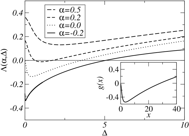
Figure 1: Lyapunov exponent $\Lambda$ of a linear, damped oscillator with parametric white noise. For different values of the control parameter $\alpha$, we plot $\Lambda$ vs. the noise amplitude $\Delta$. Inset: Graph of the function $g(x)$ (equation (13)).

External fluctuations acting upon the oscillator will first be modeled by Gaussian white noise $\xi(t)$ of zero mean value $\langle\xi(t)\rangle=0$ and of unit amplitude:

$$\langle\xi(t)\xi(t^{\prime})\rangle=\delta(t-t^{\prime})\,.$$ (9)

The stationary p.d.f. of $z$ can then be computed exactly, by adapting a calculation presented in detail in kirphil (see also tessieri ; imkeller ), where the Fokker-Planck equation equivalent to equations (7)-(9) is solved in the stationary regime. We find:

$$P_{\rm{stat}}(z)=\frac{1}{N}\int_{-\infty}^{z}\exp\left\{\frac{2}{\Delta}(\Psi(z)-\Psi(y))\right\}\mathrm{d}y,$$ (10)

where $\Psi(y)=\alpha y-\frac{1}{2}y^{2}-\frac{1}{3}y^{3}$, and $N$ is a normalisation constant. After some calculations along the lines of Ref. kirphil , equation (8) leads to the following expression for the Lyapunov exponent:

$$\Lambda(\alpha,\Delta)=\frac{1}{2}\left\{\frac{\int_{0}^{+\infty}\mathrm{d}u\;{\sqrt{u}}\;e^{\frac{2}{\Delta}\left((\alpha+\frac{1}{4})u-\frac{u^{3}}{12}\right)}}{\int_{0}^{+\infty}\frac{\mathrm{d}u}{\sqrt{u}}e^{\frac{2}{\Delta}\left((\alpha+\frac{1}{4})u-\frac{u^{3}}{12}\right)}}-1\right\}.$$ (11)

We now examine the properties of $\Lambda$ as a function of $\alpha$ and $\Delta$. We shall limit the discussion to the range $\alpha\geq-\frac{1}{4}$ (see kirphil for a detailed study of the range $(-\infty,0]$). Let $\tilde{\Delta}=\Delta/(\alpha+\frac{1}{4})^{3/2}$. We rewrite equation (11) as:

$$\Lambda(\alpha,\Delta)=\frac{1}{4}\;\sqrt{1+4\alpha}\;g(\tilde{\Delta})+\frac{1}{2}\;\left(\sqrt{1+4\alpha}-1\right),$$ (12)

where the function $g(x)$ is defined for $x\geq 0$ as

$$g(x)=\frac{\int_{0}^{+\infty}\mathrm{d}u\;{\sqrt{u}}\;e^{\frac{2}{x}\left(u-\frac{u^{3}}{12}\right)}}{\int_{0}^{+\infty}\frac{\mathrm{d}u}{\sqrt{u}}e^{\frac{2}{x}\left(u-\frac{u^{3}}{12}\right)}}-2\,.$$ (13)

The method of steepest descent yields

$$g(0)=0\,,\,\,\,\,g^{\prime}(0)=-\frac{1}{4}\,.$$ (14)

The function $g(x)$ decreases in the interval $[0,x_{m}]$, with an absolute minimum $g(x_{m})\simeq-0.54$ at $x_{m}\simeq 3.40$, then $g(x)$ increases to infinity over $[x_{m},+\infty)$ (see the inset of Fig. 1). At fixed $\alpha$, the behaviour of $\Lambda(\alpha,\Delta)$ with respect to $\Delta$ is deduced from that of $g(x)$ by translations and dilations along coordinate axes. A few representative examples are drawn in Fig. 1: $(i)$ $\alpha=-0.2$: $\Lambda$ changes sign once (noise-induced bifurcation of the nonlinear system kirphil ); $(ii)$ $\alpha=0.2$: $\Lambda$ changes sign twice (noise-induced reentrant transition of the nonlinear system); $(iii)$ $\alpha=0.5$: $\Lambda$ is positive for all $\Delta$ (no transition).

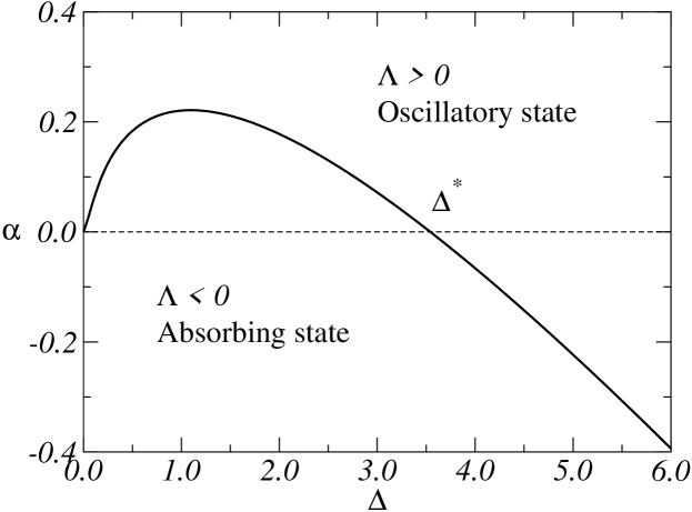
Figure 2: Bifurcation diagram of the Duffing oscillator with parametric white noise. The solid line is the locus in parameter space $(\alpha,\Delta)$ where $\Lambda(\alpha,\Delta)=0$. The bifurcation line $\alpha=0$ of the noiseless dynamical system is drawn for comparison (dotted line).

From this analysis, the bifurcation diagram of the nonlinear oscillator with parametric, Gaussian white noise (equations (3 and 9)) follows immediately. The origin is stable (resp. unstable) when the Lyapunov exponent of the linearised system is negative (resp. positive). The bifurcation line $\alpha=\alpha_{c}(\Delta)$ is defined by the equation

$$\Lambda(\alpha_{c}(\Delta),\Delta)=0\,.$$ (15)

The transition is best qualified as a stochastic Hopf bifurcation: the bifurcated state displays noisy oscillations around the origin, with a non-zero r.m.s. of the oscillator’s position and velocity. For $\Delta\leq\Delta^{*}\simeq 3.55$ (resp. $\Delta\geq\Delta^{*}$), the origin is stabilised (resp. destabilised) by the stochastic forcing in the range $0\leq\alpha\leq\alpha_{c}(\Delta)$ (resp. $\alpha_{c}(\Delta)\leq\alpha\leq 0$). The full bifurcation diagram of the inverted stochastic Duffing oscillator is displayed in Fig. 2. In the weak noise limit $\Delta\to 0^{+}$, we obtain from Eq. (14) $\alpha_{c}(\Delta)\sim(-2\;g^{\prime}(0)\;\Delta)\sim{\Delta}/{2}$, in agreement with the result of the (perturbative) Poincaré-Linstedt expansion performed in luecke .

We emphasise that the stability of the origin of the nonlinear random dynamical system (3) cannot be deduced from a stability analysis of finite-order moments of the linearised system lindenberg : indeed second-order moments of solutions of equation (5) with white noise forcing are always unstable when $\alpha$ is positive. The proper indicator of the transition of the nonlinear system is the Lyapunov exponent of solutions of the linearised equations.

Figure 3: Reentrant transition of the noisy nonlinear oscillator (3) subject to parametric white noise (9), with a fixed parameter $\alpha=0.2$. The numerical solutions of the equation $\Lambda(0.2,\Delta)=0$ are $\Delta_{1}\simeq 0.627$, $\Delta_{2}\simeq 1.700$. Even-order moments $\langle x^{2}\rangle$, $\langle x^{4}\rangle$ and $\langle x^{6}\rangle$ are plotted versus the distance to threshold $\epsilon=(\Delta_{1}-\Delta)/\Delta_{1}$ (symbols). Dashed lines respecting a linear behaviour $\langle x^{2n}\rangle\propto\epsilon^{1}$ are drawn to guide the eye. Linear scaling is also observed for the second transition ($\Delta\gtrsim\Delta_{2}$; not shown). Inset: the mean square position (measured in the stationary regime) is non-zero for $\Delta\in[0,\Delta_{1}[\cup]\Delta_{2},+\infty[$.

As an example, we show in Fig. 3 numerical evidence of a reentrant transition observed for $\alpha=0.2$. The asymptotically stable state is the origin when the noise amplitude belongs to the bounded interval $\Delta\in[\Delta_{1},\Delta_{2}]$, where $\Delta_{1}$ and $\Delta_{2}$ are the two solutions of $\Lambda(\alpha=0.2,\Delta)=0$. Noisy oscillations are found for both weaker ($\Delta<\Delta_{1}$) and stronger ($\Delta>\Delta_{2}$) noise strengths. As predicted in kirphil , even-order moments of the position and velocity scale linearly with the distance to threshold in the vicinity of these stochastic bifurcations. (Note that odd-order moment are equal to zero by symmetry.)

Since the locus of the transition is determined by a dynamical property of the linearised system, it cannot depend on the precise functional form of the confining potential ${\mathcal{U}}(x)$ for large $x$. For instance, the bifurcation line is unchanged when the confining potential reads:

$${\mathcal{U}}(x)=-\frac{1}{2}\alpha x^{2}-\frac{1}{4}x^{4}+\frac{1}{6}x^{6}\,,$$ (16)

i.e., when the deterministic nonlinear system undergoes a backward pitchfork bifurcation. We checked numerically that such is indeed the case.

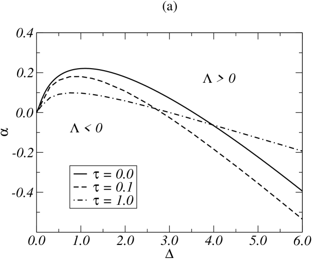
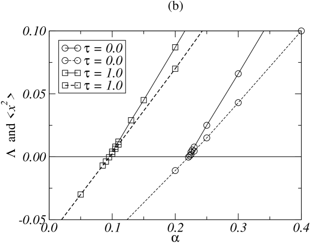
Figure 4: Parametric forcing with Ornstein-Uhlenbeck noise of correlation time $\tau$. $(a)$ Bifurcation lines for $\tau=0.1$ and $1.0$ are obtained from numerical measurements of the Lyapunov exponent (6). For comparison, we draw the (analytic) white noise line already given in Fig. 2. $(b)$ For $\tau=1.0$ and $0.0$ (white noise), we plot on the same graph, for a fixed value $\Delta=1.096$, and with respect to $\alpha$, the numerical values of the Lyapunov exponent of the linear system (symbols with dashed lines) and of the averaged square position in the oscillatory regime of the nonlinear system (symbols with solid lines). The bifurcation occurs where the Lyapunov exponent changes sign. Note the linear dependence of $\langle x^{2}\rangle$ on distance to threshold.

Let us now turn to stochastic forcing by coloured noise. For definiteness, we shall use an Ornstein-Uhlenbeck process $\xi(t)$ of correlation time $\tau$, defined as the solution of the stochastic differential equation:

$$\frac{{\textrm{d}}\xi(t)}{{\textrm{d}}t}=-\frac{1}{\tau}\xi(t)+\frac{1}{\tau}\eta(t)\,,$$ (17)

where $\eta(t)$ denotes Gaussian white noise with zero mean and unit amplitude ($\langle\eta(t)\eta(t^{\prime})\rangle=\,\delta(t-t^{\prime})$). The analytic expression of the stationary (marginal) p.d.f. $P_{\mathrm{stat}}(z)$ associated with the linear system (7-17) is not known: the Lyapunov exponent must be evaluated numerically. The line $\alpha=\alpha_{c}(\Delta)$ with $\Lambda(\alpha_{c}(\Delta),\Delta)=0$ is drawn in Fig. 4.a for $\tau=0.1$ and $1.0$. (We checked that the same measurement protocol, when used with white noise forcing, yields data in agreement with the analytic result (11).) Numerical simulations confirm that, with parametric coloured noise, $(i)$ bifurcations of the nonlinear system (equations (3-17)) occur where the Lyapunov exponent of the linear system changes sign; $(ii)$ averaged observables scale linearly with distance to threshold close to the bifurcation (see Fig. 4.b). In the weak noise limit, our data agrees with the prediction of luecke : $\alpha_{c}(\Delta)\sim\Delta/(2(1+\tau))$. For a noise amplitude of order 1, the bifurcation line is qualitatively similar to that obtained with white noise. However, depending on the value of $\Delta$, the value of the bifurcation point $\alpha_{c}(\Delta)$ is not necessarily a monotonic function of $\tau$.

We have shown here that noise can suppress oscillations by stabilizing a deterministically unstable fixed point. Our study can be related to similar observations in the context of chaotic systems where Lyapunov exponents also play a crucial role as indicators of transitions pikoskylett . Indeed, the effective lowering of Lyapunov exponents by noise can induce synchronization in a pair of chaotic systems banavar ; sanchez , or suppress chaos in nonlinear oscillators rajasekhar or in neural networks molgedey .

Our hope is that this work will help to bridge the gap between the abstract theory of random dynamical systems arnold and experimental investigations of the stability of physical systems subject to random forcing fauve ; petrelis . The behaviour of Lyapunov exponents of the linearised stochastic system (or “sample stability”) is known to explain the stability properties of a regular state of electrohydrodynamic convection of nematic liquid crystals driven by multiplicative, dichotomous noise behn . A non-perturbative study of bifurcations of spatially-extended systems under stochastic forcing of arbitrary strength kramer remains a challenging open problem.

References

- (1) L.D. Landau, E.V. Lifchitz, Mechanics (Pergamon Press, Oxford, 1969)
- (2) R. Graham, A. Schenzle, Phys. Rev. A 26, 1676 (1982)
- (3) M. Lücke, F. Schank, Phys. Rev. Lett. 54, 1465 (1985); M. Lücke, in Noise in Dynamical Systems, Vol. 2: Theory of Noise-Induced Processes in Special Applications, edited by F. Moss, P.V.E. Mc Clintock (Cambridge University Press, Cambridge, 1989)
- (4) P.S. Landa, A.A. Zaikin, Phys. Rev. E 54, 3535 (1996)
- (5) K. Mallick, P. Marcq, Eur. Phys. J. B 36, 119 (2003)
- (6) H. Horsthemke, R. Lefever, Noise Induced Transitions (Springer-Verlag, Berlin, 1984)
- (7) L. Arnold, Random Dynamical Systems (Springer-Verlag, Berlin, 1998)
- (8) C. van den Broeck, J.M.R. Parrondo and R. Toral, Phys. Rev. Lett 73, 3395 (1994)
- (9) L. Schimansky-Geier, H. Herzel, J. Stat. Phys. 70, 141 (1993)
- (10) L. Tessieri, F.M. Izrailev, Phys. Rev. E 62, 3090 (2000)
- (11) P. Imkeller, C. Lederer, Dyn. Systems 16, 29 (2001)
- (12) B.J. West, K. Lindenberg, V. Seshadri, Physica A 102, 470 (1980); K. Lindenberg, V. Seshadri, B.J. West, Phys. Rev A 22, 2171 (1980); Physica A 105, 445 (1981)
- (13) A.S. Pikovsky, Phys. Lett. A 165, 33 (1992)
- (14) A. Maritan, J.Y. Banavar, Phys. Rev. Lett. 72, 1451 (1994); A.S. Pikovsky, Phys. Rev. Lett. 73, 2931 (1994)
- (15) E. Sanchez, M.A. Matias, V. Pérez-Muñuzuri, Phys. Rev. E 56, 4068 (1997)
- (16) S. Rajasekhar, M. Lakshmanan, Physica A 167, 793 (1990); Physica D 67, 282 (1993)
- (17) L. Molgedey, J. Schuchhardt, H. G. Schuster, Phys. Rev. Lett. 69, 3717 (1992)
- (18) R. Berthet, S. Residori, B. Roman, S. Fauve, Phys. Rev. Lett. 33, 557 (2002); R. Berthet, A. Petrossian, S. Residori, B. Roman, S. Fauve, Physica D 174, 84 (2003)
- (19) F. Pétrélis, S. Aumaître, Eur. Phys. J. B 34 281 (2003)
- (20) U. Behn, A. Lange, T. John, Phys. Rev. E 58, 2047 (1998)
- (21) A. Becker, L. Kramer, Phys. Rev. Lett. 73, 955 (1994); Physica D 90, 408 (1996); J. Röder, H. Röder, L. Kramer, Phys. Rev. E 55, 7068 (1997)