Scaling law for seismic hazard after a main shock

Abstract

After a large earthquake, the likelihood of successive strong aftershocks needs to be estimated. Exploiting similarities with critical phenomena, we introduce a scaling law for the decay in time following a main shock of the expected number of aftershocks greater than a certain magnitude. Empirical results that support our scaling hypothesis are obtained from analyzing the record of earthquakes in California. The proposed form unifies the well-known Omori and Gutenberg-Richter laws of seismicity, together with other phenomenological observations. Our results substantially modify presently employed estimates and may lead to an improved assessment of seismic hazard after a large earthquake.

Earthquakes tend to occur in clusters scholz_2 . A large earthquake often precedes many further aftershocks, some of which may themselves be consequential. For instance, the Northridge earthquake in Southern California set off markedly increased seismic activity in the area, as apparent in the time series shown in Figure 1. In populated regions like Southern California that are prone to large magnitude events, the likelihood of occurrence of strong aftershocks requires accurate assessment in order to determine the risk of further damages reasenberg_1 ; reasenberg_2 ; jap_gov .

Earthquakes arise from a complicated nonlinear mechanics scholz_2 ; huang ; scholz_1 and individual events are not predictable geller ; nat_deb . Yet, simple scaling laws describe their statistical properties scholz_2 ; kagan ; bak_02 . Empirically, the number $n(t)$ of aftershocks occurring at time $t$ after a large magnitude event obeys the modified Omori law omori ; utsu_1 ; utsu_2

$$n(t)=\frac{K}{(c+t)^{p}}\qquad.$$ (1)

The constants $K$ and $c$ are positive, and the exponent $p$ is usually found to be close to one. The Gutenberg-Richter (GR) distribution gr for the frequency of earthquakes with magnitude greater than $m$ in a seismic region is

$${\cal N}(m)=A\>10^{-bm}\qquad,$$ (2)

where $A$ is a constant and the critical exponent $b$ typically takes a value close to one. Since the magnitude is proportional to the logarithm of the size of the earthquake, Eq. (2) describes a scale-free distribution.

Comparisons between seismicity and critical phenomena in other physical systems bak_02 ; bak ; turcotte suggest that these laws, usually considered to be independent, should connect inextricably together. Progress toward an organizing theory of seismicity could therefore emerge along lines similar to those followed in the modern approach to critical phenomena kadanoff . Here, we show that, in fact, the rate of earthquakes following a main shock obeys a unified scaling law. This law relates the expected number of aftershocks greater than a certain magnitude to the magnitude of the main shock itself, and to the time since the main shock. It interpolates between the Omori law at short times and the GR relation at late times, providing a coherent framework from which several other phenomenological observations can be deduced. In addition, the mathematical form for the rate of aftershocks differs significantly from the presently employed formula used to assess seismic hazard reasenberg_1 ; reasenberg_2 ; jap_gov .

Analysis of earthquake recurrence times use a magnitude threshold above which events are registered utsu_2 . This magnitude threshold always exists, even if not explicitly specified, due to limitations in reliably detecting all small earthquakes in a seismic region. Recently, Bak et al considered the magnitude threshold itself as a variable entering into a scaling law for waiting times between subsequent events bak_02 . As we show below, threshold variables also enter into a scaling theory for rates of aftershocks.

In order to quantify increased seismicity following a large earthquake, we separate smaller events from larger ones by imposing two different magnitude thresholds, as indicated in Figure 1. The threshold $M$ defines the large events. Earthquakes larger than magnitude $M$ are referred to as main shocks. A smaller threshold, $m$, selects the remaining events in the catalog to be counted. These remaining events, larger than magnitude $m$, are referred to as aftershocks. The quantity $R_{M,m}(t)dt$ is the average number of events in the catalog with magnitude larger than $m$ occurring in the interval $(t,t+dt)$, given that an isolated main shock of magnitude larger than $M$ occurred at $t=0$.

We analyzed the earthquake catalog of Southern California cal_cat from 1984 to 2002 in order to measure the rate $R_{M,m}(t)$. This catalog includes more than $3.5\times 10^{5}$ earthquakes. We identified all events larger than magnitude $M$ ($5.5\leq M\leq 6.5$). For each main shock, we measured, as a function of time, the rate of subsequent events larger than magnitude $m$ with $2.5\leq m\leq M-1.5$. The resulting data therefore contain background seismicity, unlike some other investigations kisslinger . The measurement of the rate following a given main shock was stopped when another event of magnitude $M$ or larger occurred. This ensures that each aftershock sequence does not include events from other main shocks. Some aftershock sequences, therefore, comprise more events and last longer than others. To avoid the effects of correlations between main shocks, we considered only isolated ones. We excluded all events that follow the second of two successive main shocks, where both main shocks occur within a time interval (of the order of $4$ months) of each other. An average over main shocks was then computed for each pair $(M,m)$ to obtain $R_{M,m}(t)$.

Depending on the value of $M$, the same earthquake becomes a main shock in one rate measurement, and an aftershock in another. For example, a magnitude $5.8$ earthquake could be an aftershock of a magnitude $6.7$ earthquake if $M=6$, but is treated as a main shock if $M=5.5$. This approach reflects the view that aftershocks do not differ from other earthquakes and can therefore lead to aftershocks themselves hough . In this way, the pattern of seismicity in space and time can be considered to be a single, hierarchically organized, critical process bak_02 ; bak .

Figure 2 shows the empirical results. At short times the rate, $R_{M,m}(t)$, approaches a universal constant value, $R_{0}\simeq 10^{-2}$, consistent with the presence of the parameter $c$ in Omori’s Law, Eq. (1). Strikingly, the rate at short times, $R_{0}$, appears to be independent of both $M$ and $m$, indicating that soon after a main shock earthquakes of all magnitudes are equally probable. This observation contrasts with the rate estimate used in Refs. reasenberg_1 ; reasenberg_2 ; jap_gov , where the rate at short times depends on both thresholds $M$ and $m$. However, the constant regime persists longer for increasing $M$ and/or for decreasing $m$. Later in time, a $1/t$ power law decay sets in. Each rate eventually reaches a stationary value at late times. The stationary rates for different thresholds $m$ agree with the GR law, and do not depend on $M$. The duration of aftershock activity, $t_{d}$, is defined as the time for the aftershock rate, $R_{M,m}(t)$, to decline to its stationary level. This level is referred to as background seismicity. Comparing Figs. 2a and 2b shows that the duration of aftershock activity increases as the magnitude threshold of the main shock $M$ increases.

All these observations can be combined into a single scaling hypothesis for $R_{M,m}(t)$

$$R_{M,m}(t)=\left(\frac{1}{t_{0}+10^{b(m-M)}\,t}\right)G(A\,10^{-bM}\,t)\qquad.$$ (3)

For $R_{M,m}(t)$ to approach a stationary value at late times, the scaling function $G(x)$ must behave as $G(x)\propto x$ for large $x$. In that case the stationary rate at late time is proportional to $10^{-bm}$, consistent with the GR law. At early times, $G(x)$ for small $x$ is evaluated. If this is constant, the first term on the right hand side of Eq. (3) controls the behavior. This term corresponds to an Omori law with $p=1$. The parameter $A$ and the critical exponent $b$ were determined from the GR relation, Eq. (2), to be $A=10^{-2\pm 0.2}\,\mbox{sec}^{-1}$ and $b=0.95\pm 0.1$ for the Southern California data set. The only remaining parameter in Eq. (3) is the time $t_{0}$.

The data collapse method can be used to test and potentially falsify Eq. 3. This is accomplished by rescaling the time, $t$ by $\left(A\,10^{-bM}\right)$ and the rate, $R_{M,m}(t)$ by $\left(t_{0}+10^{b(m-M)}\,t\right)$, to get a dimensionless scaling plot for $G(x)$. Using $t_{0}=6\,\mbox{sec}$, we find that all the curves collapse onto a single curve, as shown in Figure 3, within statistical error. The data collapse verifies our scaling hypothesis. The value of $t_{0}$ has an uncertainty; we estimate $4\,\mbox{sec}\leq t_{0}\leq 12\,\mbox{sec}$ from changes in the quality of the data collapse using different values for $t_{0}$. Evidently, $G(x)$ changes behavior at a turning point $x=x_{0}$. Two regimes are distinguished: a transient Omori limit at short times, $G(x\ll x_{0})\rightarrow const.$, and a stationary GR limit at late times, $G(x\gg x_{0})\rightarrow x$.

According to our scaling hypothesis, the duration of correlated aftershock activity depends on the threshold magnitude, $M$, of the main shock as

$$t_{d}\simeq\frac{x_{0}}{A}\,10^{bM}\qquad.$$ (4)

As $x_{0}\simeq 10^{-1}$ (see Figure 3) this implies, for example, that, on average, the excess rate of aftershocks persists for about two months following an earthquake of magnitude larger than six.

The parameter $c$ in Omori’s law is a controversial quantity in the earthquake literature utsu_2 . Reported values range from less than $0.01\,\mbox{days}$ to over $1\,\mbox{day}$. Previous investigations usually analyzed aftershock sequences following specific main shocks of interest. It was found that the value of $c$ decreases with increasing threshold magnitude $m$ of aftershocks included in the analysis. Comparing Eq. (1) with the scaling hypothesis (3), we obtain

$$c=t_{0}\,10^{b(M-m)}\qquad.$$ (5)

This sheds light on the variability of the $c$-value found in previous investigations.

The value of the time, $t_{0}$, can be related to the dimensionless variable, $x_{0}$, and the universal short time rate, $R_{0}$. Indeed the $1/t$ decay of the rate at intermediate times implies that $R_{0}\,c\simeq R_{M,m}(t_{d})\,t_{d}$. As $R_{M,m}(t_{d})\simeq A\,10^{-bm}$ and from expressions (4) and (5), it follows that

$$t_{0}\simeq\frac{x_{0}}{R_{0}}\simeq 10\,\mbox{sec}\qquad,$$ (6)

which is within the range of uncertainty previously estimated. This provides a consistency check on our statistical analysis. Conversely, the scaling behavior, Eq.  (5), of the $c$-value arises from the condition that the rate at short times $R_{0}$ is approximately independent of $M$ and $m$.

After a large earthquake, forecasts of seismic hazard provided by government agencies are based on estimates of the rate $\lambda_{M,m}(t)$ of aftershocks with magnitude greater than $m$ occurring at time $t$ after a main shock of magnitude $M$ reasenberg_1 ; reasenberg_2 ; jap_gov . Within our ansatz, the rate $\lambda_{M,m}(t)$ is

$$\lambda_{M,m}(t)=R_{M,m}(t)-R_{m}(\infty)-\frac{1}{b\ln 10}\frac{\partial R_{M,m}(t)}{\partial M}$$ (7)

where $R_{m}(\infty)$ is the background seismicity, generally not included in aftershock probability evaluation. Eq. (7) is only valid when $m<M$. It is important to underline that $\lambda_{M,m}(t)$ as derived here in Eq. (7), from an empirically tested law, Eq. (3), differs in several respects from presently employed estimates reasenberg_1 ; reasenberg_2 ; jap_gov . For example, it predicts that the rate of aftershocks at early times does not depend on the magnitude of the main shock or on the aftershock threshold (as discussed above, in this limit $\frac{\partial R_{M,m}(t)}{\partial M}\simeq 0$). On the contrary, in the stochastic model employed in reasenberg_1 ; reasenberg_2 , $\lambda_{M,m}(t)\sim 10^{b(M-m)}$ immediately after the mainshock.

In conclusion, we have introduced and tested against the record of recent earthquakes in California, a new scaling law that unifies the Omori law for aftershocks and the GR relation, previously considered to be independent. Our finding indicates a theoretical framework (scaling theory) within which the problem of earthquake occurrence should be considered. It provides an empirical characterization of earthquake statistics that will be useful to test theories and models in the future. Our results may also have practical implications, namely improved hazard assessment following a large earthquake.

Figure 1: Time series of earthquakes in Southern California in the month of January $1994$. The Northridge earthquake of magnitude $6.7$ occurred on January 17. The dashed line represents a main shock threshold $M=6$ and the dotted lines represent aftershock thresholds $m=3$, $3.5$ and $4$.

Figure 2: Average rate of aftershocks at time $t$ after a main shock in Southern California. In panel (a) the main shock has magnitude greater than $M=5.5$, in panel (b) greater than $M=6.5$. Averages are made over (a) $29$ and (b) $4$ main shocks. Symbols corresponds to different threshold magnitudes for aftershocks, respectively ($\bullet$) $m=2.5$, ($\blacksquare$) $m=3$, ($\blacklozenge$) $m=3.5$, ($\blacktriangle$) $m=4$, (+) $m=4.5$ and (*) $m=5$. The exponent of the straight line is $-1$.

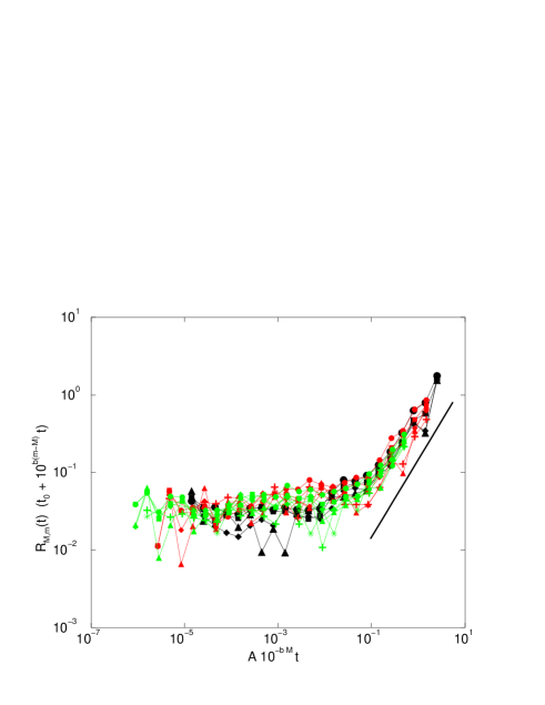
Figure 3: Data collapse for the rate of aftershocks following a main shock in Southern California. This defines the crossover function $G(x)$. The numerical values of the parameters are $b=0.95$, $A=10^{-2}\>\mbox{sec}^{-1}$ and $t_{0}=6\>\mbox{sec}$. Note that only $t_{0}$ is a fitting parameter, since the others are determined from the GR relation. Symbols are as in fig. 2, colored in black, red and green respectively for main shocks of magnitude greater than $M=5.5$, $M=6.0$ and $M=6.5$. The exponent of the straight line is $1$.

References

- (1) C. H. Scholz, The Mechanics of Earthquakes and Faulting 2nd edn (Cambridge Univ. Press, New York, 2002).
- (2) P. A. Reasenberg, L. M. Jones, Science 243, 1173 (1989).
- (3) P. A. Reasenberg, L. M. Jones, Science 265, 1251 (1994).
- (4) The Headquarters for Earthquake Research Promotion, Aftershock probability evaluation methods, http://www.jishin.go.jp/main/index-e.html (1998).
- (5) J. Huang, D. L. Turcotte, Nature 348, 234 (1990).
- (6) C. H. Scholz, Nature 391, 37 (1998).
- (7) R. J. Geller, D. D. Jackson, Y. Y. Kagan, F. Mulargia Science 275, 1616 (1997).
- (8) Nature Debates, Is the reliable prediction of individual earthquakes a realistic scientific goal?, http://www.nature.com/nature/debates/earthquake /equake_frameset.html (1998).
- (9) Y. Y. Kagan, Physica D 77, 160 (1994).
- (10) P. Bak, K. Christensen, L. Danon, T. Scanlon, Phys. Rev. Lett. 88, 178501 (2002).
- (11) F. Omori, J. Coll. Sci. Imper. Univ. Tokyo 7, 111 (1894).
- (12) T. Utsu, Geophys. Magazine 30, 521 (1961).
- (13) T. Utsu, Y. Ogata, R. S. Matsu’ura, J. Phys. Earth 43, 1 (1995).
- (14) B. Gutenberg, C. F. Richter, Bull. Seism. Soc. Am. 34, 185 (1944).
- (15) P. Bak, How Nature Works (Copernicus, New York, 1996).
- (16) D. L. Turcotte, Fractals and chaos in geology and geophysics 2nd edn (Cambridge University Press, Cambridge, 1997).
- (17) L. P. Kadanoff, Statistical Physics: Statics, Dynamics and Renormalization (World Scientific,2000).
- (18) Southern California Earthquake Data Center, http://www.scecdc.scec.org/
- (19) C. Kisslinger, L.M. Jones, J. Geophys. Res. 96, 947 (1991).
- (20) S.E. Hough, L.M. Jones, EOS, Trans. Am. Geophys. Union 78, 505 (1997).