Critical behavior near the metal-insulator transition in the one-dimensional extended Hubbard model at quarter filling

Abstract

We examine the critical behavior near the metal-insulator transition (MIT) in the one-dimensional extended Hubbard model with the on-site and the nearest-neighbor interactions $U$ and $V$ at quarter filling using a combined method of the numerical diagonalization and the renormalization group (RG). The Luttinger-liquid parameter $K_{\rho}$ is calculated with the exact diagonalization for finite size systems and is substituted into the RG equation as an initial condition to obtain $K_{\rho}$ in the infinite size system. This approach also yields the charge gap $\Delta$ in the insulating state near the MIT. The results agree very well with the available exact results for $U=\infty$ even in the critical regime of the MIT where the characteristic energy becomes exponentially small and the usual finite size scaling is not applicable. When the system approaches the MIT critical point $V\to V_{c}$ for a fixed $U$, $K_{\rho}$ and $\Delta$ behave as $|\ln\Delta|^{-2}=c_{\Delta}(V/V_{c}-1)$ and $(K_{\rho}-\frac{1}{4})^{2}=c_{K}(1-V/V_{c})$, where the critical value $V_{c}$ and the coefficients $c_{\Delta}$ and $c_{K}$ are functions of $U$. These critical properties, which are known to be exact for $U=\infty$, are observed also for finite $U$ case. We also observe the same critical behavior in the limit of the MIT critical point $U\to U_{c}$ when $U$ is varied for a fixed $V$.

I Introduction

A number of theoretical studies have been made on the one-dimensional (1D) extended Hubbard model with the on-site interaction $U$ and the nearest-neighbor interaction $V$ as a simple model for quasi-1D materials [1, 2, 3, 4]. It has been reported that this model shows a rich phase diagram including the metal-insulator transition (MIT), the phase separation, the spin-gapped phase and the superconducting (SC) phase [5, 6, 7]. In particular, the MIT at quarter-filling has attracted much interest as it takes place for finite values of $U$ and $V$ in contrast to the MIT at half-filling where the system is insulating except for $U=0$. Therefore, the MIT at quarter-filling is important as a typical example of the quantum phase transition caused by the electron correlation, and have been extensively studied by many authors [7, 8, 9, 10, 11, 12, 13]. However, the critical properties of the MIT have not received so much attention as it is more difficult to investigate the system in the limit of the MIT where the characteristic energy becomes exponentially small. In this paper, we wish to study the critical behavior near the MIT which is a typical example of the quantum critical phenomena caused by the electron correlation.

The extended Hubbard model is given by the following Hamiltonian

$$H = -t\sum_{i,\sigma}(c_{i\sigma}^{\dagger}c_{i+1\sigma}+h.c.)$$ (1)

$$+ U\sum_{i}n_{i\uparrow}n_{i\downarrow}+V\sum_{i,\sigma\sigma^{\prime}}n_{i\sigma}n_{i+1\sigma^{\prime}},$$ (2)

where $c^{\dagger}_{i\sigma}$ stands for the creation operator of an electron with spin $\sigma$ at site $i$ and $n_{i\sigma}=c_{i\sigma}^{\dagger}c_{i\sigma}$. $t$ represents the transfer energy between the nearest-neighbor sites and is set to be unity ($t$=1) in the present study. It is well known that this Hamiltonian (1) can be mapped on an $XXZ$ quantum spin Hamiltonian in the limit $U\rightarrow\infty$. The term of the nearest-neighbor interaction $V$ corresponds to the $Z$-component of the antiferromagnetic coupling and the transfer energy $t$ does the $X$-component. When the $Z$-component is larger than the $X$-component, the system has a ”Ising”-like symmetry and an excitation gap exists. For the Hubbard model, this corresponds to the case with $V>2t$ where the charge gap is exactly obtained [14]. On the other hand, in the case with ”$XY$”-like symmetry ($V<2t$), the system is metallic and the Luttinger-liquid parameter $K_{\rho}$ is exactly given by $\cos(\frac{\pi}{4K_{\rho}})=-V/2$[15].

In the finite $U$ case, exact results have not been obtained except for $V=0$. In this case, the weak coupling renormalization group method (known as $g$-ology) and the exact (numerical) diagonalization (ED) method have been applied. The $g$-ology yields the phase diagram of the 1D extended Hubbard model analytically, but quantitative validity is guaranteed only in the weak coupling regime [1, 2, 12, 13]. On the other hand, the numerical approach is a useful method to examine properties of the model in the strong coupling regime [4, 5, 6, 7, 8, 9, 10, 11]. In particular, the numerical diagonalization of a finite-size system has supplied us with reliable and important information [5, 6, 7, 8, 9, 10].

However, it is difficult for purely numerical approaches to investigate the critical behavior near the MIT where the characteristic energy scale of the system becomes exponentially small. To overcome this difficulty, we have recently proposed a combined approach of the ED and the RG methods. [9, 10]. This approach enables us to obtain accurate results of the Luttinger-liquid parameter $K_{\rho}$ and the charge gap $\Delta$ near the MIT beyond the usual finite size scaling for the ED method. The obtained results of $K_{\rho}$ and $\Delta$ have been compared with the available exact results for $U=\infty$ and found to be in good agreement [10]. The phase diagram of the MIT at quarter-filling together with the contour map of the charge gap $\Delta$ has been obtained on the $U$-$V$ plane [10]. However, the critical behavior near the MIT was not discussed in the previous work. Here we extensively apply this approach to the critical regime of the MIT to elucidate the critical behavior of $K_{\rho}$ and $\Delta$ in the limit of the MIT.

II Luttinger liquid and RG method

First, we briefly discuss a general argument for 1D-electron systems based on the bosonization theory [1, 2, 3]. According to this theory, the effective Hamiltonian can be separated into the charge and spin parts. So, we turn our attention to only the charge part and do not consider the spin part in this work. In the low energy limit, the effective Hamiltonian of the charge part is given by

$$H_{\rho} = \frac{v_{\rho}}{2\pi}\int_{0}^{L}{\rm d}x\left[K_{\rho}(\partial_{x}\theta_{\rho})^{2}+K_{\rho}^{-1}(\partial_{x}\phi_{\rho})^{2}\right]$$ (3)

$$+ \frac{2g_{3\perp}}{(2\pi\alpha)^{2}}\int_{0}^{L}{\rm d}x\cos[\sqrt{8}\phi_{\rho}(x)]$$ (4)

where $v_{\rho}$ and $K_{\rho}$ are the charge velocity and the coupling parameter, respectively. The operator $\phi_{\rho}$ and the dual operator $\theta_{\rho}$ represent the phase fields of the charge part. $g_{3\perp}$ denotes the amplitude of the umklapp scattering and $\alpha$ is a short-distance cutoff.

In the Luttinger liquid theory, some relations have been established as universal relations in one-dimensional models.[3] In the model which is isotropic in spin space, the critical exponents of various types of correlation functions are determined by a single parameter $K_{\rho}$. It is predicted that the SC correlation is dominant for $K_{\rho}>1$ (the correlation function decays as $\sim r^{-(1+\frac{1}{K_{\rho}})}$), whereas the CDW or SDW correlations are dominant for $K_{\rho}<1$ (the correlation functions decay as $\sim r^{-(1+K_{\rho})}$) in the Tomonaga-Luttinger liquid [3]. The critical exponent $K_{\rho}$ is related to the charge susceptibility $\chi_{c}$ and the Drude weight $D$ by

$$K_{\rho}=\frac{1}{2}(\pi\chi_{c}D)^{1/2},$$ (5)

with $D=\frac{\pi}{N_{a}}\frac{\partial^{2}E_{0}(\phi)}{\partial\phi^{2}}$, where $E_{0}(\phi)$ is the total energy of the ground state as a function of a magnetic flux $N_{a}\phi$ and $N_{a}$ is the system size [3]. Here, the magnetic flux is imposed by introducing the following gauge transformation: $c_{m\sigma}^{\dagger}\to e^{im\phi/N_{a}}c_{m\sigma}^{\dagger}$ for an arbitrary site $m$.

When the charge gap vanishes in the thermodynamic limit, the uniform charge susceptibility $\chi_{c}$ is obtained from

$$\chi_{c}=\frac{4/N_{a}}{E_{0}(N_{e}+2,N_{a})+E_{0}(N_{e}-2,N_{a})-2E_{0}(N_{e},N_{a})},$$ (6)

where $E_{0}(N_{e},N_{a})$ is the ground state energy of a system with $N_{a}$ sites and $N_{e}$ electrons. Here, the filling $n$ is defined by $n=N_{e}/N_{a}$.

We numerically diagonalize the Hamiltonian Eq. (1) up to 20 sites system using the standard Lanczos algorithm. Using the definitions of Eqs. (3) and (4), we calculate $D$ and $\chi_{c}$ from the ground state energy of the finite size system. To carry out a systematic calculation, we use the periodic boundary condition for $N_{e}=4m+2$ and the antiperiodic boundary condition for $N_{e}=4m$, where $N_{e}$ is the total electron number and $m$ is an integer. This choice of the boundary condition removes accidental degeneracy so that the ground state might always be a singlet with zero momentum.

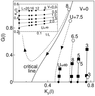
FIG. 1.: The RG flow obtained from the numerical initial condition (solid lines) and that from the analytical one (broken lines) for various $U$ at $V=0$. The filled squares are the numerical initial conditions with $L_{1}=8$ and $L_{2}=12$, and the open circles are the analytical ones. The filled diamonds on the $K_{\rho}$ axis are the exact results for $U=$3, 5, 8 and $\infty$. Inset shows the RG flow of $K_{\rho}(\ell)$ (solid lines), the numerical result of $K_{\rho}(\ell)$ (filled circles) and the exact result (filled diamonds) for various $V$ at $U=\infty$.

At quarter filling, the $8k_{F}$ umklapp scattering is crucial to understanding the MIT. The effect of the umklapp term is renormalized under the change of the cutoff $\alpha\rightarrow{\rm e}^{\ell}\alpha$. In this work, we adopt the Kehrein’s formulation as the RG equations [16, 17]

$$\frac{{\rm d}K_{\rho}(\ell)}{{\rm d}\ell} = -8\frac{G(\ell)^{2}K_{\rho}(\ell)^{2}}{\Gamma(8K_{\rho}(\ell)-1)},$$ (7)

$$\frac{{\rm d}\log G(\ell)}{{\rm d}\ell} = [2-8K_{\rho}(\ell)],$$ (8)

where the scaling quantity $\ell$ is related to the cutoff $\alpha$, $\Gamma(x)$ is $\Gamma$-function and $G(0)=g_{3\perp}/2\pi\alpha^{2}v_{\rho}$. This formulation is an extension of the perturbative RG theory and allows us to estimate the charge gap together with $K_{\rho}$ in the infinite size system. To solve these equations concretely, we need an initial condition for the two values: $K_{\rho}(0)$ and $G(0)$. Here, the value of the short-distance cutoff $\alpha$ is selected to a lattice constant of the system and set to be unity. Although the continuum field theory does not give this cutoff parameter, our choice is quite natural to apply this method to the lattice system.

In the weak-coupling limit, analytic expressions for the initial condition have been obtained [13]. At quarter filling, $v_{\rho}$, $g_{3\perp}$ and $K_{\rho}(0)$ are given by $\{(2\pi v_{F}+U+4V)^{2}-(U+4V)^{2}\}^{1/2}/2\pi$, $(U-4V)U^{2}/(2\pi v_{F})^{2}$ and $\{1+(U+4V)/(\pi v_{F})\}^{-1/2}$, respectively, where $v_{F}$ is $2t\sin k_{F}$. When we substitute these values into the RG equations as the initial condition, we find the insulating states for $U\stackrel{{\scriptstyle>}}{{{}_{\sim}}}8$ at $V=0$ in contrast to the exact results which show the metallic states for all $U$ at $V=0$. This inconsistency suggests that the analytical initial condition is not applicable in the strong coupling regime.

To find an adaptable initial condition to the strong coupling regime, we diagonalize a $L$-site system numerically and calculate $K_{\rho}(\ell)$ by using the relation $\ell\simeq\ln L$. It is easy for the numerical calculation to obtain $K_{\rho}(\ell)$ as compared to $G(\ell)$. Therefore, we calculate $K_{\rho}(\ell_{1})$ and $K_{\rho}(\ell_{2})$ with $L_{1}$- and $L_{2}$-site systems instead of $K_{\rho}(\ell)$ and $G(\ell)$ with a $L$-site system. To eliminate $G(\ell)$ in the RG equations, we integrate the Eq. (6) and obtain,

$$G(\ell)=G(\ell_{0})e^{\int_{\ell_{0}}^{\ell}[2-8K_{\rho}(\ell^{\prime})]d\ell^{\prime}},$$ (9)

where $\ell_{0}$ is a constant. Then the differential equation for $K_{\rho}(\ell)$ is written by

$$\frac{{\rm d}K_{\rho}(\ell)}{{\rm d}\ell}=-8\frac{G^{2}(\ell_{0})e^{\int_{\ell_{0}}^{\ell}[4-16K_{\rho}(\ell^{\prime})]d\ell^{\prime}}K_{\rho}(\ell)^{2}}{\Gamma(8K_{\rho}(\ell)-1)}.$$ (10)

When we set $\ell_{0}=\ell_{1}$ and use $K_{\rho}(\ell_{1})$ as the initial condition for the above equation, we can obtain the solution numerically except the constant $G(\ell_{1})$. By fitting the value of this solution at $\ell=\ell_{2}$ to $K_{\rho}(\ell_{2})$, we can determine $G(\ell_{1})$. Then, $G(\ell)$ is immediately calculated from Eq. (7) and the solution of the RG equations is completely obtained.

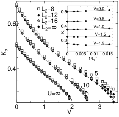
FIG. 2.: $K_{\rho}^{L_{2}}(\infty)$ as a function of $V$ at $U=5$ $10$ and $\infty$ with the exact result at $U=\infty$ (the solid line). The broken lines are guides for the eye for the data of $K_{\rho}^{\infty}(\infty)$ . Inset shows $K_{\rho}^{L_{2}}(\infty)$ as a function of $1/L_{2}^{2}$ for various $V$ at $U=\infty$ (filled circles) together with the exact result (filled diamonds).

III detailed analysis of $K_{\rho}$

In Fig. 1, we show the RG flow obtained by solving the RG equations with the numerical and the analytical initial conditions on the $K_{\rho}(\ell)$-$G(\ell)$ plane. Here, we set $L_{1}=8$ and $L_{2}=12$ for the numerical initial condition. In the weak coupling regime with $U\stackrel{{\scriptstyle<}}{{{}_{\sim}}}5$, the renormalized $K_{\rho}(\infty)$ obtained from both the initial conditions agree with the Bethe ansatz result. On the other hand, in the strong coupling regime with $U\stackrel{{\scriptstyle>}}{{{}_{\sim}}}5$, there is a large discrepancy between $K_{\rho}(\infty)$ with the analytical initial condition and the exact result. This is a striking contrast to the numerical initial condition which yields $K_{\rho}(\infty)$ in excellent agreement with the exact result even in the limit $U\rightarrow\infty$.

In the inset of Fig. 1, we plot the RG flow of $K_{\rho}(\ell)$ as a function of $L^{-1}$ for various $V$ at $U=\infty$ together with $K_{\rho}(\ell)$ from the numerical diagonalization for several system sizes $L$ and from the exact results for $L=\infty$. The RG flow seems to connect smoothly the numerical results and the exact result. It indicates that the size dependence of $K_{\rho}(\ell)$ is well described by the RG equations. For $U=\infty$, our result is consistent with the previous result from Emery and Noguera [18]. They solved the RG equations with the numerical initial conditions $K_{\rho}(\ell)$ and $G(\ell)$ for a system size $L$, where $G(\ell)$ is calculated from the excited state energy. On the other hand, in our approach, we need only the value of $K_{\rho}(\ell)$ which is calculated from the ground state. Then, our approach can be easily extended to a complicated model such as the extended Hubbard model with finite $U$ in contrast to the previous approach [18] which has been applied only for the infinite $U$ case.

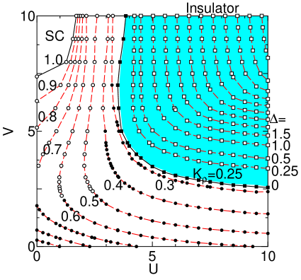
FIG. 3.: The contour lines for $K_{\rho}^{\infty}(\infty)$ and for the charge gap on the $U$-$V$ plane. The sold circles are $K_{\rho}^{\infty}(\infty)$ from the RG equations with numerical initial conditions, and the open circles are the numerical diagonalization results (see in the text). The open squares represent the charge gap (Ref. 10), whose values are 0.25, 0.5, 1, 1.5, 2, 2.5, 3, 3.5, 4, 4.5, 5 and 5.5. The filled squares represent the phase boundary of the MIT where $K_{\rho}^{\infty}(\infty)=1/4$.

In order to check the dependence of $K_{\rho}(\infty)$ on the system sizes $L_{1}$ and $L_{2}$ for the initial condition, we calculate $K_{\rho}(\infty)$ by using the three different sizes $L_{2}=8$, $12$ and $16$ with $L_{1}=L_{2}-4$. In Fig. 2, we show $K_{\rho}(\infty)$ as a function of $V$ for $U=5$, $10$ and $\infty$ together with the exact result for $U=\infty$. The value of $K_{\rho}(\infty)$ is slightly dependent on $L_{2}$. The inset in Fig. 2 shows the $L_{2}$ dependence of $K_{\rho}(\infty)$ for various $V$ at $U=\infty$ together with the corresponding exact result. Here, we assume that the size dependence of $K_{\rho}(\infty)$ is given by $K_{\rho}^{L_{2}}(\infty)\sim K_{\rho}^{\infty}(\infty)+c_{1}/L_{2}^{2}+c_{2}/L_{2}^{4}$, where $c_{1}$ and $c_{2}$ are constants, and $K_{\rho}^{\infty}(\infty)$ is the $L_{2}\to\infty$ extrapolated value of $K_{\rho}(\infty)$. We see that $K_{\rho}^{\infty}(\infty)$ is very close to the exact result for $U=\infty$. We may expect that the RG equations with numerical initial conditions give a reliable estimate for $K_{\rho}^{\infty}(\infty)$ not only for the infinite $U$ case but also for the finite $U$ case where the exact result is not known so far.

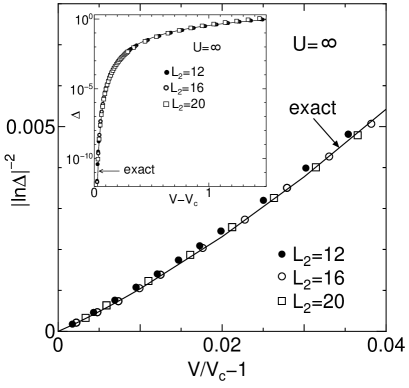
FIG. 4.: $|\ln\Delta|^{-2}$ as a function of $(V/V_{c}-1)$ near the MIT at $U=\infty$ for $L_{2}=12$, 16 and 20 together with the exact result (solid line). Inset shows $\Delta$ as a function of $V-V_{c}$.

When the strength of $V$ exceeds a critical value $V_{c}$, $K_{\rho}(\infty)$ is renormalized to the value of the strong coupling limit: $K_{\rho}=1/4$. This critical point corresponds to the MIT point of the system. In the infinite $U$ case, we find $V_{c}\simeq 1.93,1.95$ and $1.96$ for $L_{2}=12,16$ and $20$, respectively. Assuming the size dependence of $V_{c}$ to be $\propto 1/L_{2}^{2}$, we obtain an $L_{2}\to\infty$ extrapolated value $V_{c}=1.99$. It agrees well with the exact value $V_{c}=2$ for $U=\infty$. The similar extrapolation yields the critical values of the MIT: $V_{c}\simeq 3.45$ for $U=5$ and $V_{c}\simeq 2.55$ for $U=10$ as shown in Fig. 2 [20]. The results are in good agreement with the phase boundary of the MIT in the previous works [5, 6, 7, 8, 9, 10]. Then it confirms that the combined approach of the ED and the RG methods gives accurate results of $K_{\rho}$ even near the MIT.

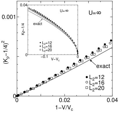
FIG. 5.: $(K_{\rho}-1/4)^{2}$ as a function of $(1-V/V_{c})$ near the MIT at $U=\infty$ for $L_{2}=12$, $16$ and $20$ together with the exact result (solid line). Inset shows $K_{\rho}-1/4$ as a function of $V-V_{c}$.

In Fig. 3, we show the phase diagram of the MIT on the $U$-$V$ plane together with the contour lines for $K_{\rho}^{\infty}(\infty)$ in the metallic region. We also plotted the contour lines for the charge gap in the insulating region which have already been reported in our previous paper [10, 19]. When $V\gg U$, the SC phase with $K_{\rho}>1$ appears. The character of this phase has already been discussed in the previous works [5, 6, 7, 8]. Near the SC phase, $K_{\rho}(\ell_{2})$ is larger than $K_{\rho}(\ell_{1})$ for available finite size systems and, then, we could not obtain the solution of the RG equations for these initial conditions. Because the umklapp scattering is canceled by the SC fluctuation, the RG equations may not be applicable in this region. Thus we estimate $K_{\rho}$ for $V\gg U$ directly by the ED method without the use of the RG method.

FIG. 6.: $|\ln\Delta|^{-2}$ as a function of $(V/V_{c}-1)$ near the MIT at $U=10$ and $U=5$ with $L_{2}=12$ and $16$ together with the straight lines whose slope are $0.20$ for $U=10$ and $0.22$ for $U=5$. Here, the factor of $\Delta$ is determined by fitting $\Delta$ to the numerical result at $V-V_{c}=1$.

FIG. 7.: $(K_{\rho}-1/4)^{2}$ as a function of $(1-V/V_{c})$ near the MIT at $U=10$ and $U=5$ for $L_{2}=12$ and $16$ together with the straight lines whose slope are $0.019$ at $U=10$ and $0.032$ at $U=5$.

FIG. 8.: $|\ln\Delta|^{-2}$ and $(K_{\rho}-1/4)^{2}$ as a function of $|U/U_{c}-1|$ near the MIT at $V=5$ for $L_{2}=12$ and $16$ together with the straight lines whose slope are $0.37$ for $|\ln\Delta|^{-2}$ and $0.050$ for $(K_{\rho}-1/4)^{2}$. Here, the factor of $\Delta$ is determined by fitting $\Delta$ to the numerical result at $U-U_{c}=1$.

IV Critical behavior near the MIT

Now we examine the critical behavior of the renormalized $K_{\rho}$ and the charge gap $\Delta$ near the MIT. In the perturbative RG approach[8, 21], the asymptotic behavior of $\Delta$ is determined by the correlation length $\xi$ as $\Delta\sim v_{\rho}/\xi$, where $\ln\xi\propto t^{-1/2}$ and $t=(\lambda-\lambda_{c})/\lambda_{c}$. Here, $\lambda$ is a relevant parameter of a model indicating the deviation from the critical point $\lambda_{c}$. The critical behavior of $K_{\rho}$ is also obtained as $(K_{\rho}-1/4)^{2}\propto t$ by analyzing the solution of the RG equations on the fixed line at $G(\infty)=0$ with $K_{\rho}\geq 1/4$.[21]

However, the derivation of $\xi$ in the perturbative RG approach is not clear because this approach leads the running coupling constants $G(\ell)$ and $K_{\rho}(\ell)$ into divergence in the gapfull region with $K_{\rho}<1/4$. Further, the perturbative RG method fails to determine the explicit values of the prefactors of ’$t^{-1/2}$’ and ’$t$’ in the formulation of $\ln\xi$ and $(K_{\rho}-1/4)^{2}$, respectively.

On the other hand, in the combined approach of the ED and the Kehrein’s RG methods, we can explicitly determine these factors without ambiguity. To avoid the difficulty of the divergence, Kehrein [16, 17] introduced a renormalized coupling constant $\tilde{G}(\ell)$ constructed by the product of $G(\ell)$ and the effective energy scale $e^{-\ell(2-8K_{\rho})}$. In the limit $\ell\to\infty$, $G(\ell)$ diverges in proportional to $e^{\ell(2-8K_{\rho})}$ (see Eq. (9)), while $\tilde{G}(\ell)$ remains a finite value and is related to the charge gap as

$$\Delta=cv_{\rho}\tilde{G}(\infty),$$ (11)

where $c$ is a factor of the order of unity. Here, the explicit value $c$ is estimated by fitting the RG result of $\tilde{G}(\infty)$ to the ED result of $\Delta$ and $v_{\rho}$ is calculated by the ED method.[22] The critical behavior of $\Delta$ including the explicit value of the prefactor is determined by $\tilde{G}(\infty)$ and the critical behavior of $K_{\rho}$ is obtained straightforwardly from the running coupling constant $K_{\rho}(\infty)$.

A $V$-dependence for $U=\infty$

First, we examine the critical behavior near the MIT for $U=\infty$, where the MIT takes place when $V$ is varied. In this case, we can test the reliability of our approach by comparing with the available exact results. Figure 4 shows the critical behavior of the charge gap $\Delta$ calculated from the combined approach of the ED and the RG methods with $L_{2}=12$, 16 and 20 at $U=\infty$, where $|\ln\Delta|^{-2}$ is plotted as a function of $(V/V_{c}-1)$ together with the exact result. In the inset in Fig. 4, $\Delta$ is plotted as a function of $V-V_{c}$. Here, the factor $c$ in Eq. (11) is determined by fitting the RG result of $\Delta$ to the numerical result from the ED method at $V-V_{c}=1$, where the system is away from the critical regime of the MIT and the ED method without the RG method can give an accurate result of $\Delta$.

As shown in Fig. 4, the critical behavior from our approach agrees very well with the exact result which is given by

$$\frac{1}{|\ln\Delta|^{2}}=c_{\Delta}\left(\frac{V}{V_{c}}-1\right),$$ (12)

for $0<(V/V_{c}-1)\ll 1$, where $c_{\Delta}=\frac{8}{\pi^{4}}$ [14]. From the results shown in Fig. 4, we estimate the coefficient as $c_{\Delta}\sim 0.087$, $0.084$ and $0.082$ for $L_{2}$=12, 16 and 20, respectively. Assuming the size dependence as $\propto 1/L_{2}^{2}$, we obtain an $L_{2}\to\infty$ extrapolated value $c_{\Delta}\sim 0.080$ which is close to the exact result of $c_{\Delta}=\frac{8}{\pi^{4}}\simeq 0.0821$. Thus, in contrast to the perturbative RG method, our approach gives reliable and explicit estimates for the charge gap $\Delta$ with very small energy scale near the MIT.

Fig. 5 shows $(K_{\rho}-1/4)^{2}$ as a function of $(1-V/V_{c})$ at $U=\infty$ calculated from our approach together with the exact result. In the critical regime, our result agrees very well with the exact result which is given by

$$\left(K_{\rho}-\frac{1}{4}\right)^{2}=c_{K}\left(1-\frac{V}{V_{c}}\right),$$ (13)

for $0<(1-V/V_{c})\ll 1$, where $c_{K}=\frac{1}{8\pi^{2}}$. From the results shown in Fig. 5, we estimate the coefficient as $c_{K}\sim 0.016$, $0.015$ and $0.014$ for $L_{2}=12$, $16$ and $20$, respectively. Using $1/L_{2}^{2}$ extrapolation, we obtain the coefficient in $L_{2}\to\infty$ as $c_{K}\sim 0.013$ which is again close to the exact result $c_{K}=\frac{1}{8\pi^{2}}\simeq 0.0127$. This indicates that our approach gives an accurate estimate for $K_{\rho}$ as well as for $\Delta$ even near the MIT beyond the usual finite size scaling for the numerical diagonalization method.

B $V$-dependence for finite $U$

Next, we examine the critical behavior of $\Delta$ and $K_{\rho}$ in the finite $U$ case. In this case, there is no available exact result. In Fig. 6, we plot $|\ln\Delta|^{-2}$ as a function of $(V/V_{c}-1)$ near the MIT for $U=10$ and $5$. We find that the critical behavior for both $U=10$ and $5$ is the same as that for $U=\infty$ given in Eq. (12) except the value of the coefficient $c_{\Delta}$. For $U=10$, we estimate the coefficient as $c_{\Delta}\sim 0.15$ and $0.15$ for $L_{2}=12$ and $16$, respectively, which yield an $L_{2}\to\infty$ extrapolated value $c_{\Delta}\sim 0.15$. For $U=5$, the values of the coefficient are $c_{\Delta}\sim 0.17$ and $0.18$ for $L_{2}$=12 and 16, respectively, resulting in an $L_{2}\to\infty$ extrapolated value $c_{\Delta}\sim 0.19$.

Fig. 7 shows the critical behavior of $K_{\rho}$ for $U=10$ and $U=5$. We again find that the critical behavior for both $U=10$ and $5$ is the same as that for $U=\infty$ given in Eq. (13) except the value of the coefficient $c_{K}$. We estimate the values of $c_{K}$ for $U=10$ as $c_{K}\sim 0.022$ and $0.022$ for $L_{2}$=12 and 16, respectively. For $U=5$, the values of the coefficient are $0.028$ and $0.029$ for $L_{2}$=12 and 16, respectively. These results yield $L_{2}\to\infty$ extrapolated values $c_{K}\sim 0.022$ for $U=10$ and $c_{K}\sim 0.030$ for $U=5$.

When $U$ decreases from $U=\infty$, both $c_{\Delta}$ and $c_{K}$ monotonically increase and become considerably large for a suitable value of $U$ such as $U=10$ and $5$ as compared to the corresponding values of $c_{\Delta}$ and $c_{K}$ for $U=\infty$.

C $U$-dependence for finite $V$

In the large $V$ regime ($V>U$), the MIT takes place at a critical value $U_{c}$ when $U$ is varied for a fixed value of $V$ as found in Fig. 3. Finally, we examine the critical behavior in this case. In Fig. 8, $|\ln\Delta|^{-2}$ and $(K_{\rho}-1/4)^{2}$ are plotted as functions of $|U/U_{c}-1|$ near the MIT for $V=5$. We find that the critical properties as functions of $U/U_{c}$ are the same as those as functions of $V/V_{c}$ given in eqs. (10) and (11) except the values of the coefficients: $|\ln\Delta|^{-2}=c^{\prime}_{\Delta}(U/U_{c}-1)$ and $(K_{\rho}-\frac{1}{4})^{2}=c^{\prime}_{K}(1-U/U_{c})$ in the limit $U\to U_{c}$, respectively. We estimate the coefficients as $c^{\prime}_{\Delta}\sim 0.30$ and $c^{\prime}_{K}\sim 0.041$ for $L_{2}=12$ and $c^{\prime}_{\Delta}\sim 0.33$ and $c^{\prime}_{K}\sim 0.046$ for $L_{2}=16$, which yield $L_{2}\to\infty$ extrapolated values as $c^{\prime}_{\Delta}\sim 0.37$ and $c^{\prime}_{K}\sim 0.050$, respectively. Both of $c^{\prime}_{\Delta}$ and $c^{\prime}_{K}$ are considerably larger than the corresponding values of $c_{\Delta}$ and $c_{K}$.

V Summary and discussion

In summary, we studied the critical behavior near the MIT in the one-dimensional extended Hubbard model at quarter filling by using the combined approach of the ED and the RG methods. In the large $U$ regime ($U>V$), the MIT takes place at a critical value $V_{c}$ when $V$ is varied for a fixed $U$, while, in the large $V$ regime ($V>U$), it takes place at a critical value $U_{c}$ when $U$ is varied for a fixed $V$. We examined the critical behavior near the MIT for both cases.

In the large $U$ regime, we observed the critical behavior, $|\ln\Delta|^{-2}=c_{\Delta}(V/V_{c}-1)$ and $(K_{\rho}-\frac{1}{4})^{2}=c_{K}(1-V/V_{c})$, where the critical value $V_{c}$ and the coefficients $c_{\Delta}$ and $c_{K}$ are functions of $U$. For $U=\infty$, the estimated values of $V_{c}$, $c_{\Delta}$ and $c_{K}$ agree well with the exact results. When $U$ decreases from $U=\infty$, all of $V_{c}$, $c_{\Delta}$ and $c_{K}$ monotonically increase. Both of $c_{\Delta}$ and $c_{K}$ become considerably large for a suitable value of $U$ such as $U=10$ and $5$ as compared to the corresponding values of $c_{\Delta}$ and $c_{K}$ for $U=\infty$.

In the large $V$ regime, we also observed the same critical properties, $|\ln\Delta|^{-2}=c^{\prime}_{\Delta}(U/U_{c}-1)$ and $(K_{\rho}-\frac{1}{4})^{2}=c^{\prime}_{K}(1-U/U_{c})$. Both of $c^{\prime}_{\Delta}$ and $c^{\prime}_{K}$ are considerably larger than the corresponding values of $c_{\Delta}$ and $c_{K}$. For $V\gg U$, the SC phase with $K_{\rho}>1$ appears. Near the SC phase, it is difficult to obtain the solution for the RG equation, because the umklapp scattering is canceled by the SC fluctuation. To examine the critical behavior near the MIT for $V\gg U$, we need an improved RG approach which includes both effects of the umklapp scattering and the SC fluctuation.

We also obtained the phase diagram on the $U-V$ plane and found that the phase boundary of the MIT and the contour lines of $\Delta$ and $K_{\rho}$ near the MIT smoothly connect between the large $U$ regime and the large $V$ regime. Although it is difficult to analyze the critical behavior for $V\gg U$, there is no qualitative difference in the critical behavior. These results suggest that the nature of the MIT is essentially unchanged on the $U-V$ plane over the whole parameter regime including the large $U$ and the large $V$ regimes.

In the limit $V=\infty$, electrons are completely inhibited to occupy the nearest neighbor site of each other. In this case, some exact results have been obtained in the previous works[5, 6, 7, 8]: the ground state energy is always zero for $U>U_{c}(=4)$ and the charge gap is given by $\Delta=|U-U_{c}|$. Then, the critical behavior of $\Delta$ for $V=\infty$ is completely different from that for finite $V$ case obtained here. We think that there are two possibilities to explain this differences as follows: (1) The critical behavior near the MIT changes discontinuously at a finite $V$. (2) The critical region smoothly shrinks with increasing $V$ and finally becomes zero in the limit $V=\infty$ where the different critical behavior is observed. In any case, the critical behavior near the MIT for $V\gg U$ is interesting problem as the competition between the SC fluctuation and the umklapp scattering becomes important, and will be studied in the future.

- [1] V. J. Emery, in Highly Conducting One-Dimensional Solids, edited by J. T. Devreese, R. Evrand and V. van Doren, (Plenum, New York, 1979), p.327.
- [2] J. Sólyom, Adv. Phys. 28, 201 (1979).
- [3] J. Voit: Rep. Prog. Phys. 58, 977 (1995).
- [4] H. Q. Lin and J. E. Hirsch, Phys. Rev B33, 8155 (1985).
- [5] F. Mila and X. Zotos, Europhys. Lett. 24, 133 (1993).
- [6] K. Sano and Y. Ōno, J. Phys. Soc. Jpn. 63, 1250 (1994).
- [7] K. Penc and F. Mila, Phys. Rev. B 49, 9670 (1994).
- [8] M. Nakamura, Phys. Rev. B 61, 16377 (2000). He shows the phase boundary of the MIT by observing the level crossing of the excitation spectra of finite size systems.
- [9] K. Sano and Y. Ōno, J. Phys. Chem. Solids. 62, 281 (2001).
- [10] K. Sano and Y. Ōno, J. Phys. Chem. Solids. 63, 1567 (2002).
- [11] Y. Shibata, S. Nishimoto and Y. Ohta, Phys. Rev. B64, 235107 (2001).
- [12] M. Tsuchiizu, H. Yoshioka and Y. Suzumura, Physica B284-288, 1547 (2000).
- [13] H. Yoshioka, M. Tsuchiizu and Y. Suzumura, J. Phys. Soc. Jpn. 69, 651 (2000).
- [14] C. N. Yang and C. P. Yang, Phys. Rev. 151, 258 (1966).
- [15] A. Luther and Peschel, Phys. Rev. B 9, 2911 (1974).
- [16] S. Kehrein, Phys. Rev. Lett. 83, 4914 (1999).
- [17] S. Kehrein, Nucl.Phys. B592, 512 (2001).
- [18] V. J. Emery and C. Noguera, Phys. Rev. Lett. 60 (1988) 631; They evaluated the umklapp scattering by the level splitting of a finite size system and calculated the Luttinger-liquid parameter from the RG equations in the limit .
- [19] The charge gap is determined by where is the total energy of the ground state for a system with electrons and is calculated up to 16 sites systems. The size dependence of is assumed as where and are constants.
- [20] In the case of , we estimate and for and 16, respectively. For , and 3.57 for and 16, respectively.
- [21] J. M. Kosterlitz, J. Phys. C7, 1046 (1974).
- [22] The value of is determined by using the relation of .