Moving and staying together without a leader

Abstract

A microscopic, stochastic, minimal model for collective and cohesive motion of identical self-propelled particles is introduced. Even though the particles interact strictly locally in a very noisy manner, we show that cohesion can be maintained, even in the zero-density limit of an arbitrarily large flock in an infinite space. The phase diagram spanned by the two main parameters of our model, which encode the tendencies for particles to align and to stay together, contains non-moving “gas”, “liquid” and “solid” phases separated from their moving counterparts by the onset of collective motion. The “gas/liquid” and “liquid/solid” are shown to be first-order phase transitions in all cases. In the cohesive phases, we study also the diffusive properties of individuals and their relation to the macroscopic motion and to the shape of the flock.

1 Introduction

The emergence of collective motion of self-propelled organisms (bird flocks, fish schools, herds, slime molds, bacteria colonies, etc.) is a fascinating phenomenon which attracted the attention of (theoretical) physicists only recently ([1, 2, 4, 5, 6]). Particularly intriguing are the situations where no “leader” with specific properties is present in the group, no mediating field helps organizing the collective dynamics (e.g. no chemotaxis), and interactions are short-range. In this case, even the possibility of collective motion may seem surprising.

However “simple” the involved organisms may be, they are still tremendously complex for a physicist and his inclination will often be to go away from the detailed, intricate, as-faithful-as-possible modeling approach usually taken by biologists, and to adopt “minimal models” hopefully catching the crucial, universal properties which may underlie seemingly different situations.

In this setting, the organisms can be reduced to points which move at finite velocity and interact with neighbors. This is in fact what Vicsek and collaborators did when introducing their minimal model for collective motion.

2 Vicsek’s model

Vicsek’s model [2] consists in pointwise particles labeled by $i$ which move synchronously at discrete timesteps $\Delta t$ by a fixed distance $v_{0}$ along a direction $\theta_{i}$. This angle is calculated from the current velocities of all particles $j$ within an interaction range $r_{\rm 0}$, reflecting the only “force” at play, a tendency to align with neighboring particles:

$$\theta_{i}^{t+1}=\arg\left[\sum_{j\sim i}\vec{v}_{j}^{t}\right]+\eta\,\xi_{i}^{t}\;,$$ (1)

where $\vec{v}_{i}^{t}$ is the velocity vector of magnitude $v_{0}$ along direction $\theta_{i}$ and $\xi_{i}^{t}$ is a delta-correlated white noise ($\xi\in[-\pi,\pi]$). Fixing $r_{\rm 0}=1$, $\Delta t=1$, and choosing, without loss of generality, a value $v_{0}\Delta t<r_{\rm 0}$, Vicsek et al studied the behavior of this simple model in the two dimensional parameter space formed by the noise strength $\eta$ and $\rho$, the particle density. They found, at large $\rho$ and/or small $\eta$, the existence of an ordered phase characterized by:

$$V\equiv{\left\langle|{\langle\vec{v}_{i}^{\/t}\rangle}_{i}|\right\rangle}_{t}>0\;,$$ (2)

i.e. a domain of parameter space in which the particles move collectively.

The existence of the ordered phase was later proved analytically [7] via a continuous model for the coarse-grained particle velocity and density. Vicsek et al devoted most of their effort to studying the transition to the ordered phase [2]. They found numerically a continuous transition characterized by scaling laws and they tried to estimate the corresponding set of critical exponents.

3 Collective and cohesive motion

Vicsek’s model accounts rather well, at least at a qualitative level, for situations where the organisms interact at short distances but need not stay together. This is for instance the case of the bacterial bath recently studied by Wu and Libchaber [9].

$\Delta t$	$v_{0}$	$r_{\rm 0}$	$r_{\rm a}$	$r_{\rm e}$	$r_{\rm c}$	$\eta$
1.0	0.05	1.0	0.8	0.5	0.2	1.0

Table 1: Fixed-value parameters used in the simulations.

In this experiment, E. Coli bacteria are swimming freely within a fluid film of thickness approximately equal to their size. By seeding the system with polystyrene beads and recording the trajectories of these passive tracers, Wu and Libchaber showed that the bacteria perform superdiffusive motion crossing over to normal diffusion. We later argued that the superdiffusive behavior is likely to be due to the onset of collective motion as in Vicsek’s model [10, 11].

When the situation to be described involves the overall cohesion of the population, Vicsek’s model needs to be supplemented by a suitable feature. Indeed, an initially cohesive flock of particles will disperse in an open space. In other words, no collective motion is possible in the zero density limit of this model. In the following, we extend Vicsek’s model to account for the possible cohesion of the population of particles.

The above remark is by no means new. Early models for the collective motion of “boids” (contraction of “birdoid”, a term used by computer animation graphics specialists) do include a two-body repulsive-attractive interaction [3]. More recent works by physicists also included this ingredient, but they either comprised an extra global interaction [4], or the actual interaction range used extended over the whole flock for the sizes considered, making it effectively global [5]. Another encountered pitfall, from our point of view at least, is to enforce the cohesion by the confinement to a rather small, close, space [6].

Here we want to be, in a sense, in the least-favorable circumstances for observing collective motion: no leader in the group, strongly noisy environment and/or communications, strictly local interactions, and no confinement at all. The “minimal” model presented below is one of the simplest possible ones satisfying these constraints.

4 A minimal model

In addition to the possibility of achieving cohesion, we also want to confer a “physical” extent to the particles, a feature absent from Vicsek’s point-particles approach. Adding a Lennard-Jones-type body force $\vec{f}$ acting between each pair of particles within distance $r_{\rm 0}$ from each other offers such a possibility.

Equation (1) is then replaced by

$$\theta_{i}^{t+1}=\arg\left[\alpha\sum_{j\sim i}\vec{v}_{j}^{t}+\beta\sum_{j\sim i}{\vec{f}}_{ij}\right]+\eta\,\xi_{i}^{t}\;,$$ (3)

where $\alpha$ and $\beta$ control the relative importance of the two “forces”. The precise form of the dependence of the body force on the distance between the two particles involved is not important. It is enough to ensure a hard-core repulsion at distance $r_{\rm c}$ and an “equilibrium” preferred distance $r_{\rm e}$.

In the following, we use

$${\vec{f}}_{ij}=\vec{e}_{ij}\left\{\begin{array}[]{ll}-\infty&{\rm if}\;\;r_{ij}<r_{\rm c}\;,\\ \frac{1}{4}\frac{r_{ij}-r_{\rm e}}{r_{\rm a}-r_{\rm e}}&{\rm if}\;\;r_{\rm c}<r_{ij}<r_{\rm a}\;,\\ 1&{\rm if}\;\;r_{\rm a}<r_{ij}<r_{\rm 0}\;.\end{array}\right.$$ (4)

with $r_{ij}$ the distance between boids $i$ and $j$, $\vec{e}_{ij}$ the unit vector along the segment going from $i$ to $j$, and the numerical values $r_{\rm c}=0.2$, $r_{\rm e}=0.5$ and $r_{\rm a}=0.8$.

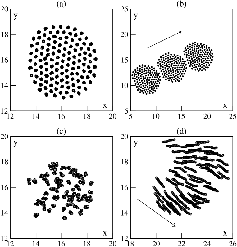
Figure 1: Cohesive flocks of 128 particles in a square box of linear size 32 with periodic boundary conditions (for parameters see Table 1). (a): immobile “solid” at $\alpha=1.0$ and $\beta=100.0$ (20 timesteps superimposed). (b): 3 snapshots, separated by 120 timesteps, of a “flying crystal” at $\alpha=3.0$ and $\beta=100.0.$ (c): fluid droplet ($\alpha=1.0$, $\beta=2.0$, 20 consecutive timesteps). (d): moving droplet ($\alpha=3.0$, $\beta=3.0$, 20 consecutive timesteps). In (b) and (d), the arrow indicates the (instantaneous) direction of motion.

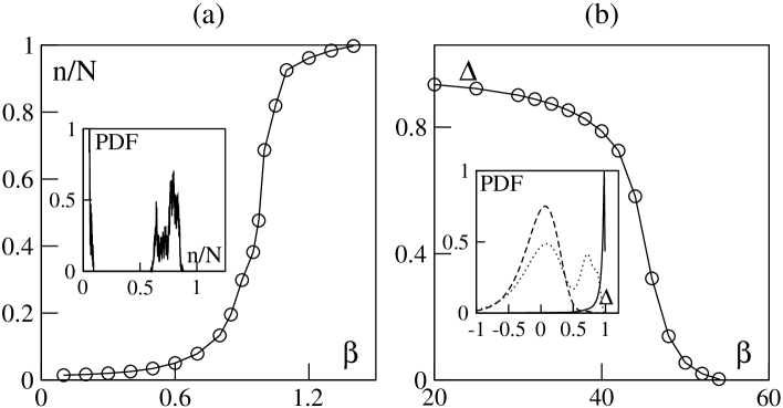
Figure 2: Order parameters at $\rho=1/16$, $L=128$, $\alpha=1.0$. (a) : “gas/liquid” transition, inset: cluster mass distribution at the coexistence point $\beta=1.0$. (b) : “liquid/solid” transition, inset: pdf of order parameter $\Delta$ for the “liquid/solid” transition, $\beta=36$ plain line (“liquid” phase), $\beta=48$ dotted line and $\beta=60$ dashed line(“solid” phase). (other parameters as in Table 1).

We have also tested other types of noise term in the model. In particular, considering the noise as the uncertainty with which each boid “evaluates” the force exerted on itself by the $N_{i}$ neighboring boids leads to change Eq. (3) to:

$$\theta_{i}^{t+1}=\arg\left[\alpha\sum_{j\sim i}\vec{v}_{j}^{t}+\beta\sum_{j\sim i}{\vec{f}}_{ij}\;+\;N_{i}\eta\vec{u}_{i}^{t}\right]$$ (5)

where $\vec{u}_{i}^{t}$ is a unit vector of random orientation. There are delicate issues related to the choice of the noise term, in particular with respect to the critical properties of the transition to collective motion [12]. We mostly considered, in the following, the noise term as prescripted above in Eq. (5). A detailed analysis of the influence of the nature of the noise is left for future studies, but we are confident that the results presented here hold generally, at least at a qualitative level.

Finally, in order to ensure that each particle only interacts with its “first layer” of neighbors (within distance $r_{\rm 0}$), we calculate, at each timestep, the Voronoi tessellation of the population [14]—this has the additional advantage of providing a natural definition of the “cells” associated with each particle. The interacting neighbors are then retricted to be those of the particles within distance $r_{\rm 0}$ which are also neighbors in the Voronoi sense.

5 Typical phases

One can easily guess the “phases” that the above model can exhibit for a fixed noise strength $\eta$ ($\eta=1.0$ in the following, for a summary of parameters see Table 1). We now present them in a qualitative manner. The results presented below were all obtained in the two-dimensional case, but most of them hold in three dimensions.

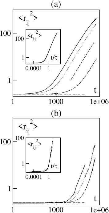
Figure 3: Mean square distance between initially-neighboring particles vs time for a flock of $10000$ boids ($L=400,\rho=1/16$) in logarithmic scales. (a) non-moving cohesive droplet ($\alpha=1.0$, $\beta=25.0$, $35.0$, $45.0$ and $150.0$ from top to bottom, the dashed line has slope 1); (b) moving cohesive flock ($\alpha=3.0$, $\beta=40.0$, $55.0$, $75.0$ and $150.0$ from top to bottom). Asymptotic transition points were measured at $\alpha=1.0$, $\beta_{\rm LS}=45.3$ and at $\alpha=3.0$, $\beta_{\rm LS}=76.1$ (see below). Other parameters as in Table 1. Insets: data collapse from which the waiting time $\tau$ can be estimated.

When the body force is weak (small $\beta$ values), the cohesion of a flock cannot be maintained. In a finite box (finite particle density $\rho$), one is left with a gas-like phase (not shown). An arbitrarily large flock in an infinite space disintegrates, eventually leaving isolated random-walking particles.

For large enough $\beta$, we can expect the cohesion to be maintained. Figure 1 shows such cohesive flocks. The internal structure of the flocks depends also on $\beta$: for large body force, positional quasi-order is present, and the particles locally form an hexagonal crystal (Fig. 1ab). For intermediate values of $\beta$, no positional order arises, and the flock behaves like a liquid droplet (Fig. 1cd).

The influence of the alignment “force” is manifested by the global motion of the flock: for large enough $\alpha$ values, the flock moves ($V>0$). Depending on $\beta$, one has then either a “moving droplet” (Fig. 1d) or a “flying crystal” (Fig. 1b).

6 Order parameters

Order parameters have to be defined to allow for a quantitative distinction between the phases described above.

The limit of cohesion separating the “liquid” phases from the “gas” can be determined by measuring the distribution of the sizes of particles clusters, thanks to an implementation of the Hoshen-Kopelman [15] algorithm. A cohesive flock is then one for which $n$, the size of the largest cluster, is of order $N$, the total number of particles. Below, we use the criterion $n/N=\frac{1}{2}$ to define the transition. Increasing $\beta$, $n/N$ sharply rises to order-one values (Fig. 2a).

The “liquid/solid” transition takes place when $\beta$ is large enough so that cohesion of the population is ensured. To determine this onset of positional quasi-order within a finite but arbitrarily large cohesive flock, we first observe that, whether in the collective motion region or not, the “liquid” and “solid” phases can be distinguished by the fact that particles diffuse with respect to each other in the “liquid”, whereas neighboring particles always remain close to each other in the “solid” (Fig. 3). To be more precise, in the “liquid”, initially close-by particles remain so for some trapping time $\tau$ (which can be defined or used to collapse the curves of Fig. 3). Approaching the “solid” phase (by increasing $\beta$), $\tau$ diverges. In addition, since we are not dealing with a translation-invariant system, we should also distinguish between the diffusion properties of the particles depending on their relative position within the flock. We have thus defined different “sectors” (“core”, “head”, “tail”, “sides”) as explained in Fig. 4.

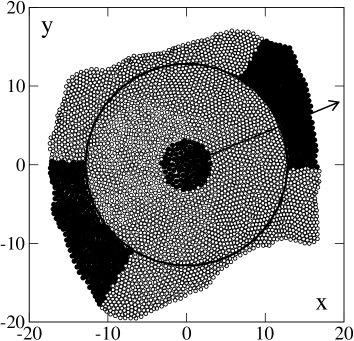
Figure 4: Snapshot of a moving flock of 4096 boids (coordinates centered on the position of the center of mass (CoM)). The arrow indicates the instantaneous direction of motion of the flock. The solid circle, centered on the CoM, has a radius equal to the root-mean-square of all boids’ distances to the CoM. The circle with a 4 times smaller radius defines the “core” region (filled circles near the CoM). The “head” contains all boids outside the larger circle which are also within a cone of opening angle $\pi/4$ centered on the direction of motion. The “tail” region is defined in an opposite manner.

If all sectors are roughly equivalent in non-moving droplets (at least sufficiently far from the “liquid/solid” transition), some differences are observed within moving droplets: the outer regions and in particular the head are more active, whereas cohesion is stronger in the core (Fig. 5). Thus, in principle, different trapping times $\tau$ can be defined for the different regions of a (moving) flock. But the depth of the outer, “more liquid”, layer does not depend on the flock size (if it is big enough), so that, in large flocks, most of the population behaves as the core. Consequently, the relative diffusion averaged over the whole flock suffers from finite-size effects, but they disappear in the large-size limit (see below). To sum up, the trapping time $\tau$ (measured on all particles of the flock) is a good quantity to track the “liquid/solid” transition. However, instead of directly estimating of $\tau$, we measured $\Delta$, the relative diffusion over some large time $T$ of initially-neighboring particles:

$$\Delta\equiv\left\langle\frac{1}{n_{i}}\sum_{j\sim i}\left(1-\frac{r_{ij}^{2}(t)}{r_{ij}^{2}(t+T)}\right)\right\rangle_{i,t},$$ (6)

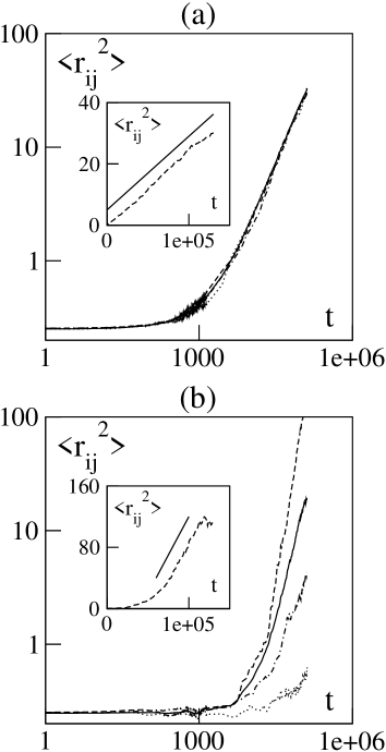
Figure 5: Growth of the mean square distance between initially-neighboring particles depending on their position within a cohesive “liquid” flock of $10000$ boids ($\rho=1/16$, $\beta=40$). (a) $\alpha=1.0$, cohesive non-moving droplet; (b) $\alpha=3.0$, moving droplet. Solid line: all boids in flock. Dotted line: core region, dashed line: head region, dash-dotted line: tail region (as defined in Fig. 4) Insets : diffusion within flock head in linear scales, the solid line is just a guide to the eye.

where the $n_{i}$ particles $j$ are the neighbors of particle $i$ at time $t$. Time $T$ is taken to be proportional to the volume of the system, which ensures that $\Delta$ records, in the large-size limit, an asymptotic property of the system (because $T\gg\tau$). Clearly, $\Delta\sim 1$ in the “liquid” phase for a large enough system, while $\Delta\sim 0$ in the “solid” phase. Indeed, increasing $\beta$, $\Delta$ falls off sharply (Fig. 2b). The transition point is chosen to be at $\Delta=\frac{1}{2}$.

Finally, we must be able to distinguish the regimes for which collective motion arises. To this aim, we use the average velocity $V$, as defined in (2). Increasing $\alpha$, $V$ reaches order-one values. The onset of collective motion is chosen to be at $V=v_{0}/2$. In the gas phase, one expects $V=0$ independently of the strengh of the alignment force. Nevertheless, this phase is rather sharply divided in two when studying the model at finite particle density. The largest cluster size may then be small ($n\ll N$), but it is (almost) always larger than one. At any given time, thus, $n>1$, and the collective motion order parameter $V$ can be defined restricted to the particles belonging to the largest cluster. (Since clusters merge and break, the particles involved generally change along time.)

7 Phase diagram

After a brief discussion of the nature of the transitions involved, we first present the phase diagram of our model for a finite density of particles in a large and fixed box size. Then we estimate finite-size effects on the location of the phase boundaries. Finally, we argue that the phase diagram can also be defined in the zero-density limit where an arbitrarily large flock wanders in an infinite space.

7.1 Nature of the transitions

As expected in usual phase transitions, we found that in our model the “gas/liquid” and “liquid/solid” transitions are first-order. In insets of Fig. 2a and b, we show the evolution of the probability distribution function of the order parameter as one crosses these transition lines. The bimodal character of these pdf at the transition is typical of first-order phase transitions, indicating the coexistence of two metastable states. At the “gas/liquid” transition point, dispersed and aggregated boids coexist and there are exchanges between the two phases along time. At the “liquid/solid” transition point, cohesion is ensured and one observes the quasi-frozen regions in an otherwise more “liquid” flock. The quasi-solid parts are often located in the core of the flock. (Fig. 6).

The nature of the transition for the onset of collective motion is a delicate issue in our model. Whereas its second-order character is rather well-established for Vicsek’s core model, we recently discovered that, in fact, the implementation of the noise term may change the nature of the transition. The detailed investigation of this, in particular in presence of the cohesive force, will be presented in a future publication [12].

7.2 Fixed population and fixed box size

A systematic scan of the ($\alpha$, $\beta$) parameter plane was performed for a flock of $N=2025$ particles living on a square surface of linear size $L=180$ ($\rho=1/16$) with periodic boundary conditions. Using the criteria defined above, we obtained the phase diagram presented in Fig. 7.

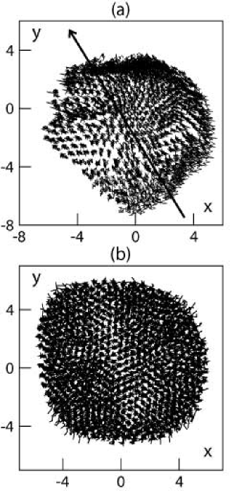
Figure 6: Short-time trajectories of freezing droplets of $N=512$ boids ($5000$ timesteps are shown, the motion of the center of mass and the solid rotation around it have been substracted). (a): in the moving phase $\alpha=3.0$, $\beta=70$: the inner part appears more solid, while the head is clearly more liquid (the arrow indicates the instantaneous direction of motion). (b): in the non-moving phase $\alpha=1.0$, $\beta=50$: one can distinguish an outer liquid layer from the almost solid core.

For each parameter value, we used an initially-aggregated flock. We let the system evolve during a time $\tau\propto L^{d}$, and then we recorded each order parameter and its histogram along time. The transition points were determined by dichotomy, the precision of which is reflected in the error bars.

The basic expected features are found: the horizontal “gas/liquid” and “liquid/solid” transitions are crossed by the vertical “moving/non-moving” line. Near this line, however, one observes a strong deformation of the “gas/liquid” and “liquid/solid” boundaries. This cannot be understood without a careful study of the collective motion transition [12].

Note also that the “gas” phase itself is crossed by the line marking the onset of collective motion, using, as explained above, the average velocity $V$ of the $n$ particles of the largest cluster as the order parameter.

7.3 Finite size and saturated vapour effects

We are ultimately interested in the possibility of collective and cohesive motion for an arbitrarily-large flock in an infinite space. The phase diagram of Fig. 7 was obtained at a fixed system size and constant density. Thus both limits of infinite-size and zero-density have to be taken to reach the asymptotic regime of interest. Of course this is mostly relevant to the onset of cohesion (the “gas/liquid” transition). Here we first study each limit separately, i.e. we investigate finite-size effects at fixed particle density and expansion at fixed particle number. Then we discuss the double-limit regime of interest.

Performing such a task for the whole parameter plane far exceeds our available computer power. We restricted ourselves to three typical cases: in the non-moving phase ($\alpha=1.0$), in the moving phase ($\alpha=3.0$) and near the transition to collective motion ($\alpha=1.75$ for the “gas/liquid” transition and $\alpha=2.1$ for the “liquid/solid” transition).

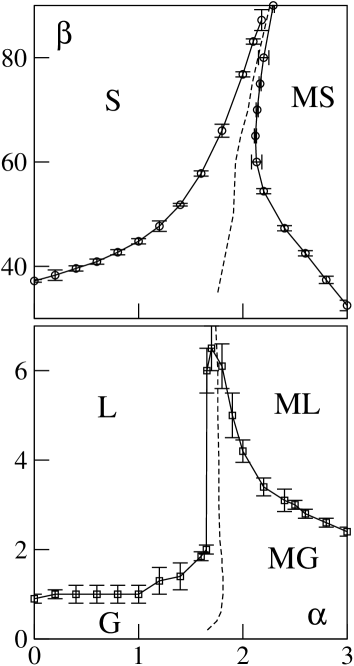
Figure 7: Phase diagram at $\rho=1/16$, $L=180$ (other parameters as in Table 1). S : solid, MS : moving solid, L : liquid, ML : moving liquid, G : gas, MG : moving gas. Dashed line : transition line of collective motion.

In simulations performed at $\rho=1/16$, varying $N$ and $L$, the transition points $\beta_{\rm GL}^{\rho}(N)$ and $\beta_{\rm LS}^{\rho}(N)$ converge exponentially as $L=\sqrt{N/\rho}$ increases. In Fig. 8, we show this for both the “gas/liquid” (a) and the “liquid/solid” (b) transitions for $\alpha=3$ (moving phases). This allows to determine asymptotic transition points. Note that exponentially-decreasing finite-size effects are typical of first order phase transition at equilibrium [16]. In the two other cases (non-moving phase, and onset of motion), the results are similar, with the asymptotic values being quickly reached in the non-moving phase ($\alpha=1$) [13].

In simulations performed at fixed $N$ varying $L$, we study instead the expansion of the system. The (finite) spatial extent induces a confinement effect which increases the pressure at the coexistence point. We thus expect a displacement of the transition point. We find that $\beta_{\rm GL}(\rho)$ also converges exponentially, and thus transition points $\beta_{\rm GL}(N)$ are well-defined. In Fig. 8c, we show this only for the “gas/liquid” transition at the $\alpha$ values used in Fig. 8a, since the “liquid/solid” transitions points were observed to be independent of the box size.

7.4 Zero-density limit

The above results provide evidence that our model possesses well-defined, asymptotic phase diagrams at either fixed particle density or at fixed number of particles. The double limit mentioned above can be approached in essentially three different ways.

One can take one limit after the other one, repeating either the calculations of Fig. 8a at lower and lower densities, or those of Fig. 8d at larger and larger flock size. However, this straightforward program involves very heavy numerical simulations. Therefore, we only considered two cases ($\alpha=1.75$ and $\alpha=3.0$). As expected, the transition points converge (exponentially) independently of the order with which the two limits are taken, yielding estimates of the zero-density limit (Fig. 9). These estimates are compatible with each other. There are three different sources of error: statistical and systematic errors when evaluating the order parameters of each system, and then fitting errors when determinating $\beta_{\rm GL}(N)$ and $\beta_{\rm GL}(\rho)$. For $\alpha=1.75$, we find a $9\%$ difference in the estimated asymptotic values whose origin is probably the statistical errors on the larger flocks simulations.

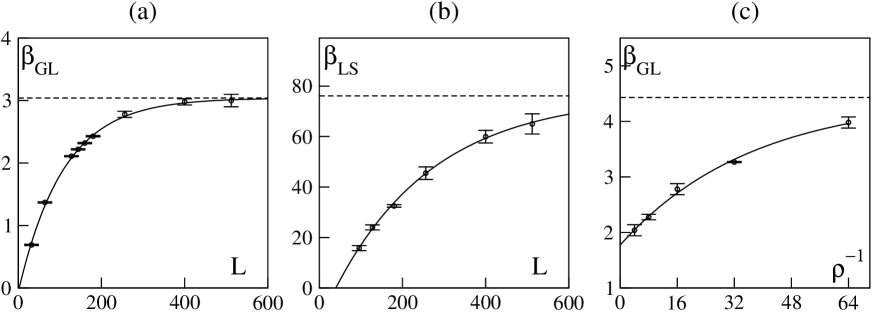
Figure 8: Finite size effects on transitions at a fixed density or at fixed number of particles at $\alpha=3.0$ (moving phases). The dashed lines are the asymptotic values determined by exponential fits (solid lines). (a) variation of the “gas/liquid” transition point $\beta_{\rm GL}$ at $\rho=1/16$ vs linear size. (b) variation of the “liquid/solid” transition point $\beta_{\rm LS}$ at $\rho=1/16$ vs linear size. (c) $\beta_{\rm GL}$ vs inverse density $1/\rho$ for $N=4096$.

7.5 Evaporation of a flock

There exists a third manner of approaching the zero-density limit of the “gas/liquid” transition. It consists in quenching a cohesive flock observed at large-enough $\beta$ to a lower $\beta$ value. If the flock is quenched below the “gas/liquid” line, it will “evaporate”.

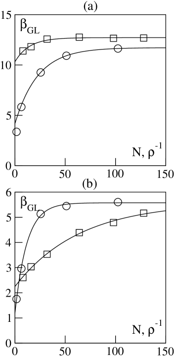
Figure 9: Zero-density limit of the cohesion transition for (a) $\alpha=1.75$ and (b) $\alpha=3.00$ (other parameters as in Table 1). Transition points at zero-density for different system sizes $N$ (circles), and at infinite-size for different (inverse) densities $\rho^{-1}$ (squares). The solid lines are exponential fits. At $\alpha=1.75$, $\beta_{\rm GL}(N)\to 11.7$ and $\beta_{\rm GL}(\rho)\to 12.7$ ; at $\alpha=3.0$, $\beta_{\rm GL}(N{\rm or}\rho)\to 5.6$.

The largest cluster will progressively lose particles before finally equilibrating in the gas phase. This transient can be expected to be governed by an effective surface tension $\gamma$ and the boundary of the largest cluster should then be governed by some Allen-Cahn law [17]: $v_{n}=\gamma\kappa$ where $v_{n}$ is the (local) normal velocity and $\kappa$ the local curvature. Assuming that the mass and the surface of the main cluster remain proportional, in the two-dimensional problem: $n=\rho_{\rm loc}\pi R^{2}$, we can integrate this equation, and we obtain the relation :

$$n=N-\lambda t\;\;{\rm with}\;\;\lambda=\pi\rho_{\rm loc}\gamma$$

where $\rho_{\rm loc}$ is the local density: the size of a circular flock should decrease linearly in time, with the proportionality constant providing an estimate of $\lambda$.

This is indeed what can be observed in our model (Fig. 10a and b). In these experiments, an initially large cohesive flock is prepared at some $\beta$ value above the transition. The system size is taken so as be close to the zero-density limit ($\rho=1/256$ in Fig. 10). We measured $T_{\rm ev}$, the time taken by the largest cluster to reach a given normalized mass $n/N$, as well as its surface at the same mass/time. We thus checked the proportionality between mass and surface and between mass and time, after transients and before the system approaches the equilibrium (Fig. 10a and b). Note that due to the abrupt change of parameters the flock actually first expands after the quench before setting in the “true” evaporation regime (Fig. 10b). This experiment can, at first sight, be thought of being free of confinement effects, and the Allen-Cahn law is expected to be satisfied at all times.

Figure 10c shows the dependence of $\lambda$ on $\beta$: $\lambda$ quickly decays and reaches very small values for $\beta\sim 0.8$. On a logarithmic scale (Fig. 10d), we can distinguish two exponential regimes, on each side of this value, which corresponds roughly to the finite-size threshold $\beta_{\rm GL}(L)$ determined above (and is rather far from the asymptotic threshold determined above to be around 1.5) A simple argument can account for this behavior: Consider a flock of $N$ boids and suppose there is no short-time expansion (such as seen in Fig. 10b). The mass of the largest cluster $n(t)$, from then on, decreases linearly with time until it reaches, at time $T_{\infty}$, the equilibrium value $n_{\rm eq}$. At every time $t$, we have:

$$N-n(t)=\frac{t}{T_{\infty}}(N-n_{\rm eq})=\lambda t\;.$$ (7)

From the theory of first order phase transitions of systems at equilibrium (see for instance [16]), we expect the order parameter $n_{\rm eq}/N$ to behave like

$$\frac{n_{\rm eq}}{N}\sim\frac{1}{2}\left[1+\tanh\left(K_{1}L^{d}(\beta-\beta_{\rm GL})\right)\right]\,,$$

in the vicinity of the transition, where $K_{1}$ is a constant. Moreover, we expect that $T_{\infty}$ depends linearly on $N$ (see Fig. 10a, where results for two different system sizes have been superimposed).

From a mean-field point of view, $T_{\infty}/N$ can be interpreted as the mean time required for a particle to escape from the interaction of another boid. Given the interaction we use (see Eq. (4)), we can assume that the potential is harmonic, so that the escape time is proportional to the exponential of the potential depth $\beta$. Finally, we get

$$\lambda \!\!\!=\!\!\! \frac{N}{T_{\infty}}\left(1-\frac{n_{\rm eq}}{N}\right)\,,\;{\rm or}$$

$$\lambda \!\!\!\propto\!\!\! \exp\left(-K_{2}\beta\right)\left[1-\tanh\left[K_{1}L^{d}\left(\beta-\beta_{\rm GL}(L)\right)\right]\right]$$

Approximating $\tanh$ by $(-1+\exp)$ and $(1-\exp)$ sufficiently far below and above $\beta=\beta_{\rm GL}(L)$, we find the two exponential regimes mentioned above. More precisely, for $\beta<\beta_{\rm GL}(L)$, the surface tension should be almost independent on system size, whereas for $\beta>\beta_{\rm GL}(L)$, $\lambda$ is governed by the finite size effects and its slope increases like $L^{d}$. Quantitative agreements with the above approximation would require too large numerical calculations, but our partial data is consistent with the above predictions.

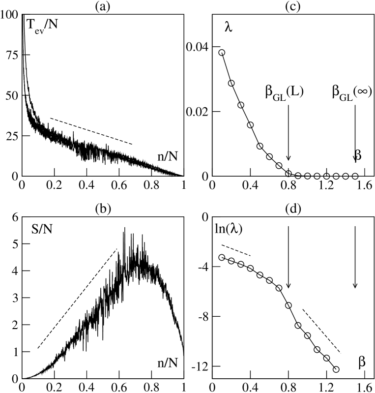
Figure 10: Evaporation at $\rho=1/256$, $\alpha=1.0$ (other parameters as in Table 1). (a) : time vs normalized cluster mass, $L=512$, and $1024$, $\beta=0.2$. (b) : surface vs normalized cluster mass, $L=512$, $\beta=0.2$. (c) surface tension vs $\beta$, in linear scale, (d) same as (c) in log-lin. scales. The dashed lines are only a guide to the eye.

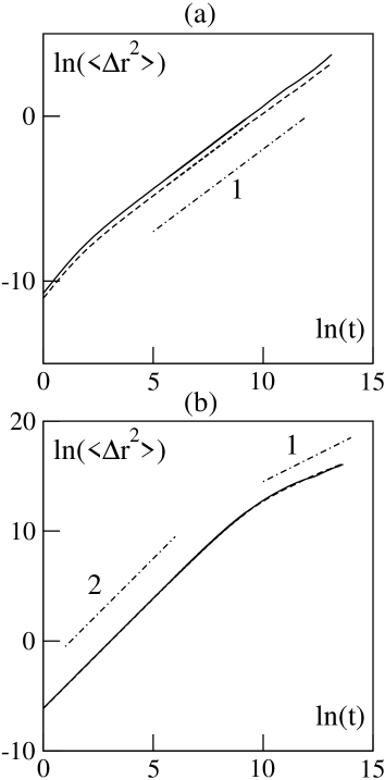
Figure 11: Mean-square displacement of the center of mass vs time for a cohesive droplet (solid lines) and for a crystal (dashed lines), $N=32$, $\rho=1/64$, logaritimic scales. (a): in the non-moving phase, $\alpha=1$, $\beta=40$ (“liquid”) and $65$ (“solid”). (b): in the moving phase, $\alpha=3$, $\beta=40$ (“liquid”) and $95$ (“solid”). The straight lines have slope 1 or 2.

A concluding remark to this investigation of the effective surface tension governing the evaporation of a flock is that, contrary to naive arguments, this method does not offer much advantage over the double-limit procedure presented in Section 7.4. Indeed, as shown above, it only allows a rather easy determination of $\beta_{\rm GL}(L)$, while the finite-size effects remain hard to estimate quantitatively.

8 Micro vs macro motion

The existence of cohesive phases being now well-established, a natural question is that of the properties of the trajectories of cohesive flocks (the “macroscopic” motion) and it is interesting to compare those to the trajectories of the individuals composing the flock (“microscopic” motion). Postponing again the account of what happens in this respect near the onset of collective motion to a further publication [12], we studied, for the four possible cohesive phases, the mean square displacement $\langle\Delta r^{2}(t)\rangle$ of the center of mass, as well as of individual boids.

Our model being essentially stochastic, it is no surprise that, at large times, we observe that $\langle\Delta r^{2}(t)\rangle\sim t$, i.e. the flock performs Brownian motion, in all cases (Fig. 11 and 12). When in a moving phase (either “liquid” or “solid”), this random walk may consist of ballistic flights separated by less coherent intervals during which the flock often changes direction. This is testified by the ballistic part ($\langle\Delta r^{2}(t)\rangle\sim t^{2}$) of the plots in Fig. 11b and by the trajectories itselves 12.

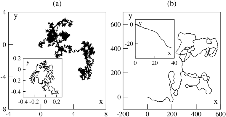
Figure 12: Trajectories of the center of mass in the non-moving phase ((a) : $\alpha=1$) and in the moving phase ((b) : $\alpha=3$). Flock of $N=32$ boids, $\rho=1/256$, $\beta=40.0$. At long times (a,b) $10^{5}$ timesteps. At short times (insets): 1000 timesteps shown.

The moving and non-moving phases can also be distinguished by opposite finite-size effects: in the non-moving phases, the diffusion constant of the macroscopic random walk decreases with system size (like $1/N$), whereas the ballistic flights’ duration increases with system size in the moving phases (Fig. 13).

Comparing the macroscopic motion of “liquid” and “solid” flocks is not well defined since, in the phase diagram, the line marking the onset of collective motion is not straight. Nevertheless, at comparable distances from this line, one notices that ballistic flights tend to be longer for flying crystals than for moving droplets. Similarly, the diffusion constant of “solid”, non-moving flocks is smaller than that of non-moving droplets.

Finally, even though we have already considered the mutual dispersion of initially-neighboring boids (see Fig. 3), we also studied the diffusive properties of individual boids within cohesive flocks, substracting out the translation motion of the center of mass. In “solid” flocks, one can hardly record any such motion. For droplets (Fig. 14), on the other hand, this microscopic motion depends on the macroscopic motion. When the droplet is fixed, the diffusion is normal $\langle\Delta r^{2}\rangle\sim t$, whereas a boid which belongs to moving flock diffuses as $\langle\Delta r^{2}\rangle\sim t^{\alpha}$, with $\alpha\sim 4/3$. We interpret this as being due to some mesoscopic “hydrodynamical” structures within moving flocks (jets, vortices, etc.). J. Toner and Y. Tu [8] have shown via a mesoscopic equation that collective motion induces transverse correlations even in a co-moving frame. Therefore, boid diffusion must be faster than Brownian. They predicted an exponent equal to $4/3$, with which our results are in good agreement (Fig. 14, top line).

9 Summary and Perspectives

We have introduced a simple model for the collective and cohesive motion of self-propelled particles. We have described its various dynamical phases, defined order parameters to distinguish them, and presented a typical phase diagram at large but finite number of particles $N$ and large but finite system size $L$ (Fig. 7). Even though we have provided evidence that this phase diagram possesses well-defined $N\to\infty$ and $L\to\infty$ limits, these limit diagrams require too heavy numerical simulations to be determined at this stage.

We have also argued that the double limit of an arbitrarily large flock evolving in an infinite space is also well-defined. Here also, the mapping of the phase diagram in this limit is currently out of reach. But the existence of cohesive phases in a model of noisy, short-range interaction, identical particles is ensured, which was one of our primary goals. Futhermore, we can sketch the zero-density asymptotic diagram from our partial knowledge (Fig. 15).

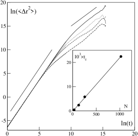
Figure 13: Mean square displacement of the center of mass vs time for a moving droplet of size $N=1024$, $256$, $128$, and $32$ from top to bottom (logarithmic scales, $\rho=1/64$, $\alpha=1.95$, $\beta=40$). The solid lines have slope 2 and 1. The larger the flock the more ballistic its motion at short times. The inset represents the cross–over time between the ballistic and the brownian motion.

A few remarks are in order to explain the expected shape of the asymptotic “gas/liquid” boundary: in the non-moving phase, this transition is almost independent on $\alpha$ and size-effects are negligible. We thus expect this line to be horizontal, in agreement with mean-field arguments (see Appendix). Similarly, our preliminary study of the onset of collective motion shows that one can go directly from a cohesive non-moving droplet to the incohesive phase and that in this region the onset of collective motion is roughly independent on $\beta$, yielding a vertical boundary.

More work should be devoted to the determination of the asymptotic phase diagrams mentioned above, as well as to a quantitative study of the onset of collective motion. Even in the simplest case of the non-cohesive Vicsek-type models, it can be second or first order, depending on the nature of the microscopic noise in the model [12]. In both cases, we have started to uncover a rich interplay between collective motion, critical fluctuations, rotation modes, and shape dynamics in the transition region.

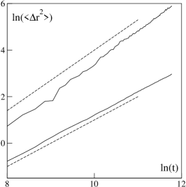
Figure 14: Internal mean-square displacement vs time of the individual boids of a cohesive droplet of 10000 boids ($\rho=1/16$, $\beta=40$, the motion of the center of mass has been substracted). Lower curve: non-moving case ($\alpha=1$), normal diffusion (the associated dashed line has slope 1). Top curve: moving case ($\alpha=3$), superdiffusion (the associated dashed line has slope 4/3, as predicted by Toner and Tu [8]).

Not even mentioning the study of our model in three dimensions and its possible applications to particular real-world situations (e.g. biology, zoology, and robotics) the work presented here is probably only the beginning of the exploration of this new type of non-equilibrium systems.

Appendix: Mean-field approach

To understand the interplay between alignment and body force, we simplify our system via a Hamiltonian model. The total energy is the sum of kinetic energy, two-body interaction energy, and a term related to the velocity alignment “force”. We thus write

$${\cal H}=\frac{Nm}{2}v_{0}^{2} \!\!\!\!+\!\!\!\! U\left(r_{1},r_{2},...,r_{N}\right)$$

$$\!\!\!\!-\!\!\!\! \alpha\sum_{i,j\sim i}^{N}\vec{v}_{i}.\vec{v}_{j}-\vec{h}_{0}.\sum_{i}^{N}\vec{v}_{i}\,.$$

where we have introduced an external field $\vec{h}_{0}$.

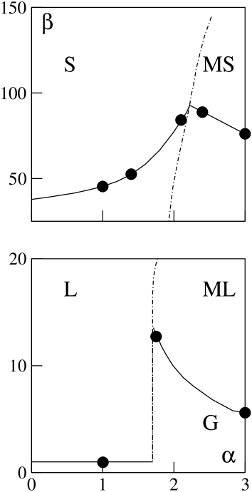
Figure 15: Sketch of the asymptotic phase diagram in the zero density limit. Filled circles indicate points determined numerically as in Section 7.4. See text for more details.

In the spirit of the mean-field approach, we assume that the fluctuations are negligible so that each component can be integrated independently and approximated by its averaged value. Thus the contibution from the two-body interaction becomes:

$$U\left(r_{1},...,r_{N}\right) \!\!\!\sim\!\!\! \frac{1}{2}\sum_{i\sim j}u\left(|\vec{r}_{i}-\vec{r}_{j}|\right)\sim\frac{N}{2}U_{0}\,,$$

$$U_{0} \!\!\!=\!\!\! \int_{R_{\rm c}}^{+\infty}\beta\rho u(r)d^{d}r\sim-2a\rho\beta\,,$$

where $a$ is a constant which depends on the potential. The alignment energy is computed with the coarse–grained velocity $\vec{\varphi}=\left<\vec{v}\right>$ and the average number of neighbors $\rho\pi r_{0}^{2}=\rho s$ :

$$\alpha\sum_{i,j\sim i}^{N}\vec{v}_{i}.\vec{v}_{j}+\vec{h}_{0}.\sum_{i}^{N}\vec{v}_{i}\sim\left(\vec{h}_{0}+\alpha\rho s\vec{\varphi}\right).\sum_{i}^{N}\vec{v}_{i}\,.$$

In the following, we use $\vec{h}_{0}+\alpha\rho s\vec{\varphi}=\vec{h}$.

Because of the separation of phase space variables, each term of the Hamiltonian contributes a factor to the partition function:
$\bullet$ the two-body coupling :

$$\left(S-bN\right)^{N}\exp\left(aN\rho\frac{\beta}{kT}\right)\,,$$ (8)

where $b=\frac{\pi}{2}R_{c}^{2}$ is the hard–core surface and $S$ is the whole surface,
$\bullet$ the alignment coupling :

$$\left[2\pi mv_{0}{\rm I_{0}}\left(-\frac{hv_{0}}{kT}\right)\right]^{N}\,,$$ (9)

where ${\rm I}_{0}$ is a Bessel function. The free energy of the system is thus written:

$$-\frac{F}{NkT}\!\!\!\! = \!\!\!\!\ln\left(\frac{mv_{0}}{\hbar}\right)-\frac{mv_{0}^{2}}{2kT}+1+\ln\left(\rho^{-1}-b\right)$$

$$+\!\!\!\! a\rho\frac{\beta}{kT}+\ln{\rm I}_{0}\left(-\frac{hv_{0}}{kT}\right)-\rho s\varphi^{2}\frac{\alpha}{2kT}$$

Imposing to be at a minimum of the free energy, we find that the average velocity is the solution of a self–consistent equation:

$$\frac{\varphi}{v_{0}}=\frac{{\rm I}_{1}}{{\rm I}_{0}}\left(\frac{v_{0}h}{kT}\right)\,,$$ (10)

and that the critical point is defined by

$$sv_{0}^{2}\rho\alpha=2kT\,.$$ (11)

Collective motion thus emerges via a continous phase transition whose critical exponents are $1/2$ for the order parameter and $1$ for its susceptibility, independently of the cohesive force.

Furthermore, the necessary concavity of the free energy function implies a first order cohesion transition, since the second derivative of the free energy has two zeros. Their positions define the phase coexistence region. We determined the stability limit of the gas phase. As positions and velocities are decorrelated, we studied two cases : first without any motion, and then with collective motion. In the first case:

$$\beta_{\rm GL}=\frac{kT}{2a\rho\left(1-b\rho\right)^{2}}\,,$$ (12)

which means that the transition line does not depend on the alignment parameter (Fig. 16). Note also that there is no transition point in the zero–density limit of this model. We numerically solved the case with collective motion and found a stabilization of the “liquid” phase (Fig. 16). This is an effect of the assumption that velocity fluctuations are negligible. At the onset of motion, we expect that fluctuations of the macroscopic velocity diverge, leading to strong density fluctuations. This could explain the de–stabilization of the “liquid” phase (Fig. 15) and its stabilization in the mean field model 16, where such fluctuations are by definition absent.

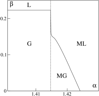
Figure 16: Phase diagram of a mean field model. L : liquid, ML : moving liquid, G : gas, MG : moving gas. Dashed line : transition line of collective motion.

References

- [1] J.K. Parrish and W.M. Hamner (Eds.), Three dimensional animals groups , Cambridge University Press (1997), and references therein.
- [2] T. Vicsek, A. Czirók, E. Ben-Jacob, I. Cohen and O. Shochet, Phys. Rev. Lett. 75, 1226 (1995). A. Czirók, H. E. Stanley, T. Vicsek, J. Phys. A 30, 1375 (1997).
- [3] C. W. Reynolds, Comput. Graph. 21, 25 (1998).
- [4] N. Shimoyama, K. Sugawara et al , Phys. Rev. Lett 76, 3870 (1996).
- [5] A. S. Mikhailov and D. H. Zanette, Phys. Rev. E 60, 4571 (1999); H. Levine, W.-J. Rappel and I Cohen, Phys. Rev. E 63, 017101 (2001); I. Couzin et al , J. theor. Biol 218, 1 (2002).
- [6] Y. L. Duparcmeur, H. Herrman and J. P. Troadec, J. Phys. I France 5, 1119 (1995); J. Hemmingson, J. Phys. A 28, 4245 (1995).
- [7] J. Toner and Y. Tu, Phys. Rev. Lett. 75, 4326 (1995); Phys. Rev. E 58, 4828 (1998)
- [8] J. Toner, Y. Tu and Ulm, Phys. Rev. Lett. 80, 4819 (1998)
- [9] X.-L. Wu and A. Libchaber, Phys. Rev. Lett. 84, 3017 (2000).
- [10] G. Grégoire, H. Chaté, and Y. Tu, Phys. Rev. Lett. 86, 556 (2001) and Phys. Rev. E 64, 011902 (2001).
- [11] X.-L. Wu and A. Libchaber, Phys. Rev. Lett. 86, 557 (2001)
- [12] G. Grégoire, H. Chaté, and Y. Tu, in preparation.
- [13] G. Grégoire, Mouvement collectif et physique hors d’équilibre, PhD thesis, Université Denis Diderot–Paris 7, Paris (2002).
- [14] A. Okabe et al, Spatial Tesselations, ed. J. Wiley and sons, ltd, Chichester (1992).
- [15] J. Hoshen and R. Kopelman, Phys. Rev. B 14, 3438 (1976)
- [16] C. Borgs and R. Koteckỳ, J. Stat. Phys. 61, 79 (1990)
- [17] See, e.g.: A.J. Bray, Adv. Phys. 43,357 (1994)