Return times of random walk on generalized random graphs

Abstract

Random walks are used for modeling various dynamics in, for example, physical, biological, and social contexts. Furthermore, their characteristics provide us with useful information on the phase transition and critical phenomena of even broader classes of related stochastic models. Abundant results are obtained for random walk on simple graphs such as the regular lattices and the Cayley trees. However, random walks and related processes on more complex networks, which are often more relevant in the real world, are still open issues, possibly yielding different characteristics. In this paper, we investigate the return times of random walks on random graphs with arbitrary vertex degree distributions. We analytically derive the distributions of the return times. The results are applied to some types of networks and compared with numerical data.

I Introduction

The theory of the random walk has a long history. Random walks and their extensions have also been applied with profound theoretical bases to modeling numerous types of physical, biological, sociological, and economical dynamics Spitzer . For example, distributions of return times and scaled limit distributions of the walkers’ positions are broadly known for simple underlying graphs. They provide useful information on critical values and phase transitions in regard to survival of the branching random walks and the contact processes Liggettbook99 ; Schinazibook ; Pemantle01 , survival in the voter models Liggettbook99 ; Durrettbook , and occurrence of percolation Lyons90_Lyons95 ,

Indeed, a large body of theoretical results are available for random walks performed on regular lattices such as ${\bf Z}^{d}$ and on the Cayley (or regular) trees, which are defined to be trees with homogeneous vertex degree. However, it has been suggested recently that more complex networks as opposed to regular graphs and conventional random graphs Erdos are concerned to real worlds. Particularly, important classes of random graphs such as small-world networks and scale-free networks were proposed and have been examined in the last several years. These networks share some important properties with real networks, such as the clustering property, short average path length, and the power-law of the vertex degree distributions SW-SF ; Callaway00 ; Albert02 ; Newman . They have been applied to the analysis of various biological, engineering, and social networks including information flow in the Internet Callaway00 ; Albert02 ; Newman and epidemics Newman ; Eguiluz_Pastor_Masuda_SARS . The properties of spatial stochastic models, both static configurations and dynamical processes, typically change as the network topology varies even when other basic quantities such as the mean vertex degree is conserved. For example, the analysis of percolation-based models revealed that the critical parameter values for the occurrence of global epidemics, or even their existence, depend on network topology Callaway00 ; Albert02 ; Newman .

It is highly likely that the properties of random walks depend on network topology Schinazibook ; Pemantle01 , as numerical and approximate results suggest for the quenched Pandit and annealed Jasch_Lahtinen Watts-Strogatz-type small-world networks and for quenched random graphs with homogeneous vertex degree Szabo00rw . In relation to this issue, how eigenvalues of the adjacency matrices are distributed has been numerically examined for scale-free and small-world networks Farkas_Goh . The largest eigenvalue of an adjacency matrix measures how the number of closed paths increases as the path length tends to infinity. The eigenvalues supply useful information on the return times of random walks Spitzer , serving to a wide range of applications as mentioned above. However, the largest eigenvalue $\rho$ has been characterized only in terms of the numerical scaling law for the scale-free networks in an unnormalized manner, namely, $\rho\propto m^{1/2}N^{1/4}$, where $N$ is the system size and $2m$ is the mean vertex degree Farkas_Goh .

In this paper, we analyze random walks on a general class of random graphs that includes random scale-free networks, the Erdös-Rényi random graph, and the Cayley trees as special cases Lyons90_Lyons95 ; Pemantle01 ; Albert02 ; Newman . Explicit expressions for the first return time probability and the annealed approximation forms for the general return time probability are derived with the use of partition of integers. In Sec. II, we introduce the network model and the generating functions. In Sec. III, we calculate the probability distribution functions of the return time of random walk. Then, in Sec. IV, we confirm with some examples that our theoretical estimates match numerical results. Lastly, the conclusion follows, and the difference in the decay rate of the return time probability between regular and random networks, which implies the difference in the possibility of percolation and the survival of contact processes, are also touched upon.

II Network Model and Generating Functions

We analyze a class of random graphs called generalized random graphs in physical contexts Callaway00 ; Albert02 ; Newman or Galton-Watson trees in mathematical contexts Lyons90_Lyons95 ; Pemantle01 . These random graphs are infinite trees without loops. The degree of each vertex, or the number of neighbors, is distributed according to an identical and independent probability density function. As shown in Fig. 1, each realization of the graph, which is generally inhomogeneous, is taken from the random ensemble. However, they are regular in a statistical sense. Let us denote by $p_{k}$ the probability that a vertex has the degree equal to $k$. We assume that $p_{0}=0$ without losing generality. Consequently, $\sum^{\infty}_{k=1}p_{k}=1$.

Let us designate an arbitrary vertex $O$ of a realized graph as the root. We examine a random walk starting from $O$. Since we exclusively deal with trees here, the random walker can return to $O$ only when the time $n\in$ $\{0,1,2,\ldots\}$ is even. In accordance, we denote by $q_{n}$ the probability that the random walker returns to $O$ for the first time at time $2n$, and by $r_{n}$ the probability that it returns to $O$ irrespective of the accumulated number of returns. Here we consider only the annealed random walk, confining ourselves in the analysis of return times averaged over both probability space of graph and that of random walk. To be contrasted with the annealed randomness is the quenched randomness, which is concerned to the ensemble of walkers on a fixed realization of random graph Zeitouni02 . Both quenched Pandit ; Szabo00rw and annealed Jasch_Lahtinen random walks have been implicitly treated in the studies of random dynamics on complex networks. Though quenched environments are realistic, the statistics based on annealed walks that we derive in the following can be regarded as averages of the statistics of quenched walks over the ensemble of a random graph.

The generating functions for the distributions $\{q_{n}\}$ and $\{r_{n}\}$, which we respectively denote by $Q(z)$ and $R(z)$ are defined by

$$Q(z)\equiv\sum^{\infty}_{n=0}q_{n}z^{n},\quad R(z)\equiv\sum^{\infty}_{n=0}r_{n}z^{n}.$$ (1)

With $q_{0}=0$ and $r_{0}=1$, $Q(z)$ and $R(z)$ satisfy the following relation:

$$R(z) = \sum^{\infty}_{n=0}\left(\sum^{n}_{m=1}q_{m}r_{n-m}+\delta_{n,0}\right)z^{n}$$ (2)

$$= R(z)Q(z)+1,$$

where $\delta_{i,j}=1$ for $i=j$ and $\delta_{i,j}=0$ otherwise Spitzer ; Grimmettbook . Strictly speaking, Eq. (2) is valid only for the quenched case. Therefore, the following results for $R(z)$ should be understood as an approximation by annealed statistics.

III Distributions of Return Times

To derive explicit expressions for the return time distributions, we provide the approximate recursion relation below. Let us resort to Fig. 1 for explanation. Suppose that the random walker starting from $O$ returns to $O$ after $2n$ steps for the first time ($n=7$ in Fig. 1). In the first step, the random walker moves to a neighbor that we denote by $O^{\prime}$. Because of the statistical homogeneity of the generalized random graph, the vertex degree of $O^{\prime}$ is distributed as specified by $\{p_{k}\}$ whichever neighbor of $O$ is chosen. The random walker has to arrive at $O^{\prime}$ at time $2n-1$ ($=13$) and move to $O$ subsequently at time $2n$ $(=14)$. The last event occurs with probability $1/k$. In the meantime, the random walker travels for $2n-2$ steps without visiting $O$. The walker wanders in the subtrees rooted at $O^{\prime}$ to complete loops, or closed paths of random walk. Any such loop cannot contain $O$, and the probability that a path emanating from $O^{\prime}$ enters a subtree is $(k-1)/k$. Let us denote by $a$ the number of the loops originating from $O^{\prime}$. In Fig. 1, $a$ is equal to 2. Then, the length $2n_{i}$ ($1\leq i\leq a$) of each loop is even ($n_{1}=5$ and $n_{2}=1$ in Fig. 1), and $2n_{i}$ must sum up to $2n-2$. In addition, since the vertex degree is homogeneously distributed, the probability law for the length of loop is assumed to be the same as that for the original random walk starting and ending at $O$.

Here we make a crucial approximation of disregarding any memory effects. In other words, we suppose that the $a$ subtrees rooted at $O^{\prime}$ are independent of each other. In fact, if the same neighbor of $O^{\prime}$ is chosen for different entries into the subtree, the subtrees reached by these different entries coincide. As an example, the random walker shown in Fig. 1 travels from $A$ to the subtree rooted at $B$ twice, before returning to $O$. In this occasion, it is not qualified to regard the vertex degrees and the loop lengths to be independent for the two neighbors of $O^{\prime}$. However, the approximation error is small unless the mean vertex degree is extremely small. The accuracy of the following analytical methods are investigated in comparison with numerical simulations in Sec. IV.

Based on the consideration above, we have the following recursion formula:

$$q_{n} = \sum^{\infty}_{k=1}p_{k}\sum^{n-1}_{a=0}\sum_{\sum^{a}_{i=1}n_{i}=n-1,n_{i}\geq 0,1\leq i\leq a}\frac{k-1}{k}q_{n_{1}}\;\frac{k-1}{k}q_{n_{2}}\;\ldots\;\frac{k-1}{k}q_{n_{a}}\;\frac{1}{k}$$ (3)

$$= \sum^{\infty}_{k=1}\frac{p_{k}}{k}\sum^{\infty}_{a=0}\left(\frac{k-1}{k}\right)^{a}\sum_{\sum^{a}_{i=1}n_{i}=n-1,n_{i}\geq 0,1\leq i\leq a}\prod^{a}_{a^{\prime}=1}q_{n_{a^{\prime}}},$$

which covers the singular case $q_{0}=0$ as well. Using Eq. (3), the generating function of $q_{n}$ is calculated as

$$Q(z) = \sum^{\infty}_{n=0}\left\{\sum^{\infty}_{k=1}\frac{p_{k}}{k}\sum^{\infty}_{a=0}\left(\frac{k-1}{k}\right)^{a}\sum_{\sum^{a}_{i=1}n_{i}=n-1,n_{i}\geq 0,1\leq i\leq a}\prod^{a}_{a^{\prime}=1}q_{n_{a^{\prime}}}\right\}z^{n}$$ (4)

$$= z\sum^{\infty}_{k=1}\frac{p_{k}}{k}\sum^{\infty}_{a=0}\left(\frac{k-1}{k}\right)^{a}\sum^{\infty}_{n=0}\sum_{\sum^{a}_{i=1}n_{i}=n-1,n_{i}\geq 0,1\leq i\leq a}\prod^{a}_{a^{\prime}=1}q_{n_{a^{\prime}}}z^{n_{a}^{\prime}}$$

$$= z\sum^{\infty}_{k=1}\frac{p_{k}}{k}\sum^{\infty}_{a=0}\left(\frac{k-1}{k}\right)^{a}Q(z)^{a}$$

$$= z\sum^{\infty}_{k=1}\frac{p_{k}}{k-(k-1)Q(z)}.$$

Although $Q(1)=1$ is always consistent with Eq. (4), we exclude this case because the random walk on generalized random graphs including the Cayley trees is transient Lyons90_Lyons95 , except for the Cayley tree with vertex degree 2, which is identical to ${\bf Z}$. Accordingly, we look for the solution satisfying $Q(1)<1$.

By expanding the right-hand side of Eq. (4), we obtain

$$Q(z) = z\sum^{\infty}_{k=1}\frac{p_{k}}{k}\sum^{\infty}_{n=0}\left(\frac{k-1}{k}Q(z)\right)^{n}$$ (5)

$$= \frac{zM\left[Q(z)\right]}{Q(z)},$$

where

$$M(z)\equiv\sum^{\infty}_{n=1}m_{n}z^{n}$$ (6)

is the generating function of the moment function given by

$$m_{n}\equiv\sum^{\infty}_{k=1}\frac{(k-1)^{n-1}}{k^{n}}\;p_{k}.$$ (7)

In deriving Eq. (5), the expansion is justified by the fact that $Q(z)$ has the radius of convergence equal to 1 and that $(k-1)/k<1$. Then, we apply the following theorem to calculate $Q(z)$ and $R(z)$.

Lagrange’s inversion formula Grimmettbook Let $z=w/f(w)$ where $w/f(w)$ is an analytic function of $w$ near $w=0$. If $g$ is infinitely differentiable, then

$$g\left(w(z)\right)=g(0)+\sum^{\infty}_{n=1}\frac{z^{n}}{n!}\left[\frac{d^{n-1}}{du^{n-1}}\left[g^{\prime}(u)f(u)^{n}\right]\right]_{u=0}.$$ (8)

For our purpose, we set $w(z)=Q(z)$, $f(w)=M(w)/w$, $g(w)=w$ in Eq. (8). Apparently, the fact that $m_{1}>0$ guarantees the regularity of $w/f(w)$ around $w=0$. As a result, we have

$$Q(z) = g(w)$$ (9)

$$= 0+\sum^{\infty}_{n=1}\frac{z^{n}}{n!}\left\{\frac{d^{n-1}}{du^{n-1}}\left[\left(\frac{M(u)}{u}\right)^{n}\right]\right\}_{u=0}.$$

We also note that

$$M(u)^{n} = (m_{1}u+m_{2}u^{2}+\cdots)^{n}$$ (10)

$$= \sum^{\infty}_{n^{\prime}=n}u^{n^{\prime}}\sum_{\lambda\vdash n^{\prime},\sum^{\infty}_{l=1}i_{\lambda}(l)=n}\frac{n!}{\prod^{\infty}_{l=1}i_{\lambda}(l)!}\prod^{\infty}_{l=1}m_{l}^{i_{\lambda}(l)},$$

where $\sum_{\lambda\vdash n^{\prime}}$ indicates the summation over all the partitions of the integer $n^{\prime}$ into integers. In general, a partition $\lambda$ is represented by $\lambda=(1^{i_{\lambda}(1)}2^{i_{\lambda}(2)}\cdots)$, which means that 1 is included $i_{\lambda}(1)$ times in $\lambda$, 2 is included $i_{\lambda}(2)$ times, and so on Stanleybook . By the definition of partition, $\{i_{\lambda}(1),i_{\lambda}(2),\ldots\}$ ($\lambda\vdash n^{\prime}$) satisfies

$$\sum^{\infty}_{l=1}l\;i_{\lambda}(l)=\sum^{n^{\prime}}_{l=1}l\;i_{\lambda}(l)=n^{\prime}.$$ (11)

For example,

$$\left\{\lambda\;|\;\lambda\vdash 5\right\} = \left\{(1^{5}),(1^{3}2),(1^{2}3),(12^{2}),(14),(23),(5)\right\},$$ (12)

$$\left\{\lambda\;|\;\lambda\vdash 7\right\} = \left\{(1^{7}),(1^{5}2),(1^{4}3),(1^{3}2^{2}),(1^{3}4),(1^{2}23),(1^{2}5),(12^{3}),(124),(13^{2}),\right.$$ (13)

$$\left.(16),(2^{2}3),(25),(34),(7)\right\}.$$

In Eq. (10), only the partitions whose numbers of parts are $n$ are concerned. Corresponding to Eqs. (12) and (13), the partitions appearing in the summation of Eq. (10) for $(n,n^{\prime})=(3,5)$ and $(4,7)$ are as follows:

$$\left\{\lambda\;\bigg{|}\;\lambda\vdash 5,\sum^{\infty}_{l=1}i_{\lambda}(l)=3\right\} = \left\{(1^{2}3),(12^{2})\right\},$$ (14)

$$\left\{\lambda\;\bigg{|}\;\lambda\vdash 7,\sum^{\infty}_{l=1}i_{\lambda}(l)=4\right\} = \left\{(1^{3}4),(1^{2}23),(12^{3})\right\}.$$ (15)

With Eq. (10), Eq. (9) is evaluated as follows:

$$Q(z) = \sum^{\infty}_{n=1}\frac{z^{n}}{n!}(n-1)!\sum_{\lambda\vdash 2n-1,\sum^{\infty}_{l=1}i_{\lambda}(l)=n}\frac{n!}{\prod^{\infty}_{l=1}i_{\lambda}(l)!}\prod^{\infty}_{l=1}m_{l}^{i_{\lambda}(l)}$$ (16)

$$= \sum^{\infty}_{n=1}z^{n}\sum_{\lambda\vdash 2n-1,\sum^{\infty}_{l=1}i_{\lambda}(l)=n}c^{(n)}_{\lambda}\prod^{\infty}_{l=1}m_{l}^{i_{\lambda}(l)},$$

where

$$c^{(n)}_{\lambda}=\frac{(n-1)!}{\prod^{\infty}_{l=1}i_{\lambda}(l)!}.$$ (17)

Accordingly,

$$q_{n}=\sum_{\lambda\vdash 2n-1,\sum^{\infty}_{l=1}i_{\lambda}(l)=n}c^{(n)}_{\lambda}\prod^{\infty}_{l=1}m_{l}^{i_{\lambda}(l)}$$ (18)

when $n\geq 1$, and $q_{0}=0$.

What is necessary for deriving $R(z)$ is just to replace $g(w)=w$ with $g(w)=1/(1-w)$ when applying Eq. (8). Using Eq. (10), we obtain the annealed approximation form of $R(z)$:

$$R(z) = \frac{1}{1-Q(z)}$$ (19)

$$= g(w)$$

$$= 1+\sum^{\infty}_{n=1}\frac{z^{n}}{n!}\left[\frac{d^{n-1}}{du^{n-1}}\left(\frac{-1}{(1-u)^{2}}\left(\frac{M(u)}{u}\right)^{n}\right)\right]_{u=0}$$

$$= 1+\sum^{\infty}_{n=1}\frac{z^{n}}{n!}\sum^{n-1}_{n^{\prime\prime}=0}\left[\frac{(-1)^{n-n^{\prime\prime}}(n-n^{\prime\prime})!}{(1-u)^{n-n^{\prime\prime}+1}}\frac{d^{n^{\prime\prime}}}{du^{n^{\prime\prime}}}\left(\frac{M(u)}{u}\right)^{n}\right]_{u=0}$$

$$= 1+\sum^{\infty}_{n=1}\frac{z^{n}}{n!}\sum^{n-1}_{n^{\prime\prime}=0}(-1)^{n-n^{\prime\prime}}(n-n^{\prime\prime})!$$

$$\times\left[\sum^{\infty}_{n^{\prime}=n+n^{\prime\prime}}\frac{(n^{\prime}-n)!}{(n^{\prime}-n-n^{\prime\prime})!}u^{n^{\prime}-n-n^{\prime\prime}}\sum_{\lambda\vdash n^{\prime},\sum^{\infty}_{l=1}i_{\lambda}(l)=n}\frac{n!}{\prod^{\infty}_{l=1}i_{\lambda}(l)!}\prod^{\infty}_{l=1}m_{l}^{i_{\lambda}(l)}\right]_{u=0}$$

$$= 1+\sum^{\infty}_{n=1}\frac{z^{n}}{(n-1)!}\sum^{n-1}_{n^{\prime\prime}=0}(-1)^{n-n^{\prime\prime}}(n-n^{\prime\prime})!\;n^{\prime\prime}!\sum_{\lambda\vdash n+n^{\prime\prime},\sum^{\infty}_{l=1}i_{\lambda}(l)=n}c^{(n)}_{\lambda}\prod^{\infty}_{l=1}m_{l}^{i_{\lambda}(l)},$$

which results in

$$r_{n}=\frac{1}{(n-1)!}\sum^{n-1}_{n^{\prime\prime}=0}(-1)^{n-n^{\prime\prime}}(n-n^{\prime\prime})!\;n^{\prime\prime}!\sum_{\lambda\vdash n+n^{\prime\prime},\sum^{\infty}_{l=1}i_{\lambda}(l)=n}c^{(n)}_{\lambda}\prod^{\infty}_{l=1}m_{l}^{i_{\lambda}(l)},$$ (20)

when $n\geq 1$, and $r_{0}=1$.

IV Examples

The analytical methods developed in Sec. III can be broadly applied since the only assumptions that we have made on $\{p_{k}\}$ are $p_{0}=0$ and that the average vertex degree is not so small. In this section, we apply our theoretical estimates to random walk on some classes of graphs that are often relevant in real-world situations and also of theoretical interest.

IV.1 Cayley trees

Let us first consider the Cayley trees Albert02 in which each vertex has exactly $d$ vertices. Substituting $p_{k}=\delta_{k,d}$ into Eq. (4) yields

$$Q(z)=\frac{1}{d-(d-1)Q(z)}.$$ (21)

Although Eq. (21) has two different solutions of $Q(z)$, the one satisfying $Q(1)=1$ is excluded because of the transient nature of the random walk on the Cayley trees Spitzer ; Lyons90_Lyons95 ; Grimmettbook . Then Eq. (21) is led to

$$Q(z)=\frac{d-\sqrt{d^{2}-4(d-1)z}}{2(d-1)}.$$ (22)

In this case, $Q(z)$ is related to the generating function $S(z)$ of Catalan numbers $D_{n}\equiv{}_{2n}C_{n}/(n+1)$ Stanleybook as follows:

$$S(z)=\frac{1-\sqrt{1-4z}}{2z}=\frac{d-1}{dz}Q\left(\frac{d^{2}}{d-1}z\right).$$ (23)

Accordingly, we obtain

$$q_{n}=\frac{(d-1)^{n-1}}{d^{2n-1}}D_{n-1}.$$ (24)

On the other hand, applying $m_{l}=(d-1)^{l-1}/d^{l}$ to Eq. (18) results in

$$q_{n} = \sum_{\lambda\vdash 2n-1,\sum^{n}_{l=1}i_{\lambda}(l)=n}c^{(n)}_{\lambda}\frac{(d-1)^{\sum^{n}_{l=1}(l-1)i_{\lambda}(l)}}{d^{\sum^{n}_{l=1}li_{\lambda}(l)}}$$ (25)

$$= \frac{(d-1)^{n-1}}{d^{2n-1}}\sum_{\lambda\vdash 2n-1,\sum^{n}_{l=1}i_{\lambda}(l)=n}c^{(n)}_{\lambda}.$$

Combining Eqs. (24) and (25) provides a useful by-product:

$$\sum_{\lambda\vdash 2n-1,\sum^{n}_{l=1}i_{\lambda}(l)=n}c^{(n)}_{\lambda}=D_{n-1},$$ (26)

which states that the sum of the coefficients in the moment expansion of $q_{n}$ [see Eq. (18)] is always equal to $D_{n-1}$ without regard to the distribution $\{p_{k}\}$.

Similarly, Eq. (19) becomes

$$R(z)=\frac{2-d+\sqrt{d^{2}-4(d-1)z}}{2(1-z)}.$$ (27)

Then, it follows that

$$\left(1-\frac{d^{2}}{d-1}z\right)R\left(\frac{d^{2}}{d-1}z\right)=1-dzS(z)$$ (28)

and

$$r_{n}=1-\sum^{n-1}_{n^{\prime}=0}\left(\frac{(d-1)^{n^{\prime}-1}}{d^{2n^{\prime}-1}}\right)D_{n^{\prime}}.$$ (29)

Owing to the entire homogeneity of the Cayley trees, Eqs. (22) and (27) are exact in this case and agree with the theoretical results obtained by identifying random walk on the Cayley trees with unbiased random walk on ${\bf Z}$ Spitzer ; Grimmettbook .

IV.2 Erdös-Rényi random graph

The Erdös-Rényi (ER) random graph is generated by independently assigning an edge with probability $p$ between any possible pairs of vertices Erdos ; Albert02 ; Newman . If the number of vertices $N$ scales so that $\lambda\equiv Np$ converges in the limit $N\to\infty$, the vertex degree is distributed as specified by the Poissón distribution, namely,

$$p_{k}=\frac{\lambda^{k}}{k!}{\rm e}^{-\lambda}.$$ (30)

Numerically calculated distributions of the first return time are indicated by circles in Figs. 2(a) and 2(b) for $\lambda=7$ and $\lambda=10$, respectively. The return probability decreases exponentially in $n$ analogous to the case of the Cayley trees indicated by solid lines in Fig. 2 Spitzer ; Schinazibook ; Grimmettbook . Then many sample points are required for reliable estimation of the return time probability, for which reason we construct the probability distributions based on $5\times 10^{7}$ runs. A new random graph is created in each run.

Distributions predicted by the theory in Sec. III are indicated by crosses in Fig. 2. The theoretical estimates agree with the numerical results better when $\lambda=10$. This is because our method works better for networks with a larger mean vertex degree, which is equal to $\lambda$. However, the error is bearable in both cases for sufficiently small $n$ for which the numerical distributions are calculated based on enough sample points. In other words, the minimum positive probability obtained by the simulations is $1/(5\times 10^{7})=2\times 10^{-8}$, and the numerically estimated probabilities are not reliable around this value where statistical fluctuation counts. Related to this remark, Fig. 2 shows that the numerical results are actually available just up to small values of $n$, that is, $n\leq 17$ for $\lambda=7$ and $n\leq 12$ for $\lambda=10$. As noted before, this is due to the exponential decay in the return time distribution. Furthermore, the decay is faster for a larger mean vertex degree, or a larger $\lambda$, which more severely constrains the practical upper limit of $n$ for which the distribution is obtained. Compared with the cumbersome brute-force method, our method needs only calculation of partition of integers, which are much more numerically feasible.

Figure 2 also shows, both for $\lambda=7$ and $\lambda=10$, that the decay of the first return time probability is slower for the ER random graphs than for the Cayley trees with the same mean vertex degree. This is presumably because of the dispersion of vertex degree in the ER random graph, as we discuss in Sec. V.

IV.3 Scale-free networks

The vertex degrees of real networks often have power-law distributions. Barabási and co-workers presented a network growth model with preferential attachment to generate such a graph SW-SF ; Albert02 . In their scale-free networks, the vertex degree has a lower cutoff $m$, and the degree distribution is represented by $p_{k}={\cal N}k^{-3}$ ($k\geq m$) and $p_{k}=0$ ($k<m$), where ${\cal N}$ is the normalization constant. The first return time probabilities of random walk on scale-free random graphs with $m=4$ are shown in Fig. 3, suggesting that the theory (crosses) again predicts the numerical results (circles) in a satisfactory manner. In this case, the mean vertex degree is numerically calculated to be 7.09. Accordingly, the results for the Cayley trees with $d=7$ (solid lines) and $d=8$ (dotted lines) are also shown in Fig. 3 for comparison. The probability of the first return time decays slower for the scale-free networks, as has also been the case for the ER random graphs. Moreover, comparison of Figs. 2 and 3 reveals that the discrepancy from the regular case, which is probably caused by the heterogeneous vertex degree, is larger for the scale-free networks. This is presumably because the vertex degree is more heterogeneous in the scale-free networks than in the ER random graphs.

Random walk on other related graphs, such as ones whose degree distributions have power laws without the lower cutoff, power laws with exponential higher cutoff, or simple exponential decay Callaway00 ; Newman , can be analyzed similarly. The only caveat is that the theory is likely to fail when the vertex degree is fairly small on average. Let us also mention that there is little hope for obtaining more tractable analytical expressions for $Q(z)$ and $R(z)$ even in simpler scale-free cases, because the polylogarithm functions, which can be estimated only numerically Newman , appear in the calculation of $m_{l}$.

V Conclusions

In this paper, we have derived for generalized random networks the analytic expressions for the probability distributions of first and general return times. Our methods correctly predict the numerical results as far as the mean vertex degree is not extremely small. They are also useful in saving the computation time and hence obtaining return time probabilities on a much longer time scale than with straightforward simulations. This merit stems from the fact that the algorithm for calculating partition of integers is easily implemented Stanleybook , whereas brute-force methods require billions of runs to obtain the distributions and the asymptotics, particularly in the case of exponentially decaying tails.

We have also found that heterogeneous graphs such as the ER random graphs and the scale-free networks yield slower decay of return time probabilities than the Cayley trees with the corresponding vertex degrees. The decay rate is closely linked to critical phenomena and phase transitions of both static Lyons90_Lyons95 and dynamical Liggettbook99 ; Schinazibook ; Pemantle01 ; Durrettbook particle systems. In social contexts, information and diseases are actually suggested to propagate in a manner different from as we imagine by the analogy of regular graphs such as the Cayley trees and regular lattices. For example, percolation is more likely to occur in networks with heterogeneous vertex degrees Newman . Also for dynamical processes such as contact processes Liggettbook99 ; Schinazibook ; Eguiluz_Pastor_Masuda_SARS and voter models Liggettbook99 ; Durrettbook , occurrence of global orders such as epidemics or unanimity has the same tendency. Mathematically, the problem of the global orders emerging in these dynamics can be associated with that of the dual or related processes. For example, if simple and branching random walks (resp. coalescing random walks) are more likely to return to the origin, the critical value for phase transition becomes smaller, and the probability of a global epidemics or unanimity becomes larger in contact processes Liggettbook99 ; Schinazibook (resp. voter models Liggettbook99 ; Durrettbook ). Accordingly, the asymptotic behavior of random walk reported in Sec. IV suggests that global orders are more likely consequences in networks with heterogeneous vertex degrees such as scale-free and ER random networks. This evidence substrates the results for the contact processes in epidemic contexts Eguiluz_Pastor_Masuda_SARS and poses a dynamical version of the exact results on percolation Newman .

As for exact asymptotic behavior, questions about the Cayley trees with vertex degree $d$ is translated into ones about the unbalanced random walk on ${\bf Z}$, the analysis of which easily resulting in $r_{n}\propto n^{-3/2}\left(2\sqrt{d-1}/d\right)^{2n}$ Schinazibook . To illuminate the asymptotic behavior of $q_{n}$ and $r_{n}$ in the case of generalized random walks is an important subject of future work.

Figure captions

Figure 1: Schematic diagram showing random walk on a realization of generalized random graph. Integers denotes the time of random walk.

Figure 2: Probability distributions of the first return times of the random walk on the ER random graph with (a) $\lambda=7$ and (b) $\lambda=10$. Numerical and theoretical results are indicated by circles and crosses, respectively. The results for the Cayley trees with the same mean vertex degrees, namely, (a) $d=7$ and (b) $d=10$, are indicated by solid lines.

Figure 3: Probability distributions of the first return times in the case of scale-free networks with $m=4$. Numerical and theoretical results are indicated by circles and crosses, respectively. The results for the Cayley trees with $d=7$ (solid lines) and $d=8$ (dashed lines) are also shown.

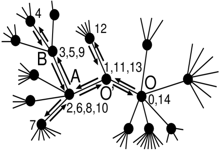
Figure 1:

Figure 2:

Figure 3: