Fcc-bcc transition for Yukawa interactions determined by applied strain deformation

Abstract

Calculations of the work required to transform between bcc and fcc phases yield a high-precision bcc-fcc transition line for monodisperse point Yukawa (screened-Couloumb) systems. Our results agree qualitatively but not quantitatively with recently published simulations and phenomenological criteria for the bcc-fcc transition. In particular, the bcc-fcc-fluid triple point lies at a higher inverse screening length than previously reported.

I Introduction

The screened-Coulomb or Yukawa pair potential, $U(r)=\Phi e^{-\kappa r}/r$, has been the focus of great theoretical interest for two reasons. One is that it describes a wide range of interactions, changing continuously from a pure Coulomb potential to an effective hard-sphere potential as the inverse screening length $\kappa$ increases. The second is that it provides an approximate description of the effective interactions between large ions that are screened by more mobile counterions. In this context it has been used to describe the interactions between ions surrounded by electrons in metals Ashcroft and Mermin (1976), dust grains surrounded by electrons in dusty plasmas Whipple et al. (1985); Hamaguchi and Farouki (1994); Rosenfeld (1994), and macroions surrounded by counterions in charge-stabilized colloidal suspensions Rosenfeld (1994); Verwey and Overbeek (1948); Alexander et al. (1984); Stevens et al. (1996); Palberg et al. (1995).

The phase diagram of systems of particles interacting with a Yukawa potential has been studied with both analytic Hone et al. (1983); Shih and Stroud (1983); Vaulina et al. (2002); Vaulina (2002); Tejero et al. (1992); Rosenberg and Thirumalai (1987) and numerical Rosenberg and Thirumalai (1987); Meijer and Frenkel (1991); Zahorchak et al. (1992); Stevens and Robbins (1993); Farouki and Hamaguchi (1994); Hamaguchi et al. (1996); Kremer et al. (1986); Robbins et al. (1988); Dupont et al. (1993); Hamaguchi et al. (1997); Miller and Reinhardt (2000) techniques and compared to experiments on dusty plasmas Chu and I (1994); et.al (2003) and colloidal suspensions Monovoukas and Gast (1989); Sirota et al. (1989); Schope et al. (1998). The high temperature phase is a fluid. There is no liquid-gas transition because the interactions are purely repulsive. The stable crystalline phase at zero temperature changes from bcc to fcc as $\kappa$ increases. The higher entropy of the bcc phase leads to a greater range of stability as temperature increases until the melting line is reached. Previous results for the fcc-bcc transition line Hone et al. (1983); Kremer et al. (1986); Robbins et al. (1988); Dupont et al. (1993); Hamaguchi et al. (1997); Miller and Reinhardt (2000) vary substantially and the most recent detailed calculation Hamaguchi et al. (1997) quotes an uncertainty of about 10% roughly halfway between the zero-temperature transition point and the triple point.

In this paper we use a different approach to obtain the bcc-fcc phase boundary with an uncertainty of only about 1%. Bounds on the free energy difference between the two phases are obtained by calculating the work done during a continuous deformation between them. The effect of deformation rate, truncation of the potential, and system size and geometry are all analyzed to determine systematic errors. The resulting bcc-fcc transition line is in qualitative agreement with recent simulation results, and quantitative differences are comparable to the larger error bars quoted by previous studies. We estimate the location of the bcc-fcc-fluid triple point using previously published melting-line results Stevens and Robbins (1993); Hamaguchi et al. (1997), and find that it lies at higher inverse screening lengths than previously reported.

The role of anharmonicity in stabilizing the fcc phase is analyzed in detail. While anharmonicity increases the energy of the fcc phase relative to that of the bcc, there is an even larger increase in the relative entropic contribution to the free energy that increases the range of stability of the fcc phase. This appears to reflect an increase in the frequency of the long wavelength shear modes that dominate the bcc entropy in the harmonic approximation Robbins et al. (1988).

Our results are also compared to phenomenological criteria proposed by Vaulina et. al. Vaulina et al. (2002). These authors predict a transition at a critical value of the mean-squared displacement about lattice sites, and calculate the displacement using a simple Einstein-like model. We find that the actual displacement from MD simulations on our transition line is in reasonable agreement with their phenomenological criterion, but substantially larger than predicted by their Einstein model.

The details of our calculations are presented in the following section. Section III provides a detailed analysis of systematic errors and presents our results for the phase boundary. In Section IV, we compare our results to previous transition lines, and Section V provides a summary and conclusions.

II Method

II.1 Free energy difference calculations

NVT ensembles are most natural for the study of Yukawa systems for two reasons. First, since the Yukawa potential is purely repulsive, the macroions in an experiment will expand to fill the container. Second, the inverse screening length $\kappa$ is density dependent in charged colloidal suspensions and dusty plasmas . This density dependence is system-specific, and affects the pressures and bulk moduli. Thus any calculation of coexistence regions will be non-universal. For this reason we focus on finding the Helmholtz free energy difference $\Delta F=F_{fcc}-F_{bcc}$ at fixed volume. A brief discussion of coexistence is given in Section II.2.

Postma, Reinhardt, and others Straatsma et al. (1986); Reinhardt and Hunter (1992); Hunter et al. (1993) have shown that the free energy difference between two phases of a system may be calculated in numerical simulations by evaluating the external work done on the system along a thermodynamic path connecting the phases. From elementary thermodynamics, the mechanical work $W_{AB}$ done on a system on an isothermal path from state A to state B gives an upper bound on the change $\Delta F_{AB}=F_{B}-F_{A}$ in the system’s Helmholtz free energy Reif (1965). The work $W_{BA}$ done on the system during the reverse process $B\to A$ is an upper bound on $\Delta F_{BA}$, and hence $(-W_{BA})$ is a lower bound on $\Delta F_{AB}$.

Bounds on $\Delta F$ for Yukawa systems can be obtained using a continuous constant-volume Bain deformation path (Fig. 1) connecting the bcc and fcc lattices. An initially bcc lattice deformed such that its three cubic symmetry directions are scaled respectively by $(\zeta^{-1/2},\zeta^{-1/2},\zeta)$ is transformed into an fcc lattice of the same density as $\zeta$ varies continuously from 1 to $2^{1/3}$ Milstein et al. (1994). We calculate the work done along this path in the forward and reverse directions using strain-controlled molecular dynamics simulations Hoover et al. (1980).

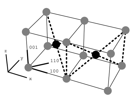
Figure 1: The Bain transformation. Two cells of a bcc lattice are shown with lattice directions. The body-center atoms are shown in black. When the x, y, and z directions are scaled by $(2^{-1/6},2^{-1/6},2^{1/3})$, the crystal is transformed into an fcc lattice of the same density. The atoms connected by the dotted lines become two (100) faces of an fcc unit cell.

Assuming that the systems traverse these paths homogeneously, we can calculate the work done from the global stresses and strains. We define

$$W_{bf}=V\int_{bcc}^{fcc}\bar{\sigma}\cdot d\bar{\epsilon},$$ (1)

$$W_{fb}=V\int_{fcc}^{bcc}\bar{\sigma}\cdot d\bar{\epsilon},$$ (2)

where $\bar{\sigma}$ and $\bar{\epsilon}$ are the stress and true strain tensors. $W_{bf}$ and $(-W_{fb})$ are upper and lower bounds on $\Delta F$. For these bounds to be narrow, the intermediate configurations of our systems must remain statistically representative of the $\zeta$-dependent equilibrium distributions as $\zeta$ is varied Straatsma et al. (1986). In particular, the stress tensor $\bar{\sigma}(\zeta)$ must remain near its equilibrium value.

II.2 Potential parameters

The phase behavior of Yukawa systems is most conveniently expressed in terms of dimensionless screening and temperature parameters. One natural, phase- independent length scale is $a=n^{-1/3}$, where $n=N/V$ is the macroion number density. The Yukawa potential may then be expressed as

$$U(r)=\frac{\Phi}{a}\frac{e^{-\lambda r/a}}{r/a},$$ (3)

where $\lambda=\kappa a$ is the dimensionless screening parameter. The limits $\lambda\to 0$ and $\lambda\to\infty$ correspond to the exhaustively studied one-component plasma and hard-sphere systems.

A natural time scale is provided by $\tau_{E}$, the period of an Einstein oscillator in a crystal. The Einstein periods for the fcc and bcc phases change by an order of magnitude over the range of $\lambda$ studied here $(3\leq\lambda\leq 8)$, yet differ from each other by less than 1.2% at any given $\lambda$ within this range. To obtain consistent results across a wide range of screening lengths, we normalize all time scales in this study to $\tau_{E}(\lambda)$, using the fcc values given in Ref. Robbins et al. (1988).

A natural energy scale is given by the Einstein phonon energies $m\omega_{E}^{2}a^{2}$, where m is the macroion mass and $\omega_{E}=2\pi/\tau_{E}$ is the Einstein frequency. Following Kremer, Robbins, and Grest Kremer et al. (1986), we define the dimensionless temperature

$$\widetilde{T}=\displaystyle\frac{k_{B}T}{m\omega^{2}_{E}a^{2}}$$ (4)

using the fcc phonon energies, and plot our phase diagram in $(\lambda,\widetilde{T})$ space. A dimensionless inverse temperature $\Gamma=(\Phi/a)/k_{B}T$ called the coupling parameter is used in many studies of dusty plasmas. The advantage of using $\widetilde{T}$ rather than $\Gamma$ in Yukawa phase diagrams is that the transition lines are approximately linear in $\lambda$.

The bcc and fcc phases coexist in equilibrium over a part of the phase diagram. Following previous authors Kremer et al. (1986); Robbins et al. (1988); Dupont et al. (1993); Hamaguchi et al. (1997), we define the bcc-fcc transition line as the curve $\widetilde{T}_{trans}(\lambda)$ on which $\Delta F=\Delta F(\lambda,\widetilde{T})=0$. This transition line will certainly lie within the coexistence region, regardless of the thermodynamic state dependence of $\kappa$ and $\Phi$. We find $\widetilde{T}_{trans}(\lambda)$ by calculating $\Delta F$ at many points $(\lambda_{i},\widetilde{T}_{i})$ on the phase diagram.

II.3 MD simulation details

We simulate NVT ensembles of identical particles using a velocity-Verlet Swope et al. (1982) algorithm to integrate the particle trajectories. The temperature is maintained with a Langevin thermostat Schneider and Stoll (1978). Periodic boundary conditions are used to maintain the density. The equations of motion for the position $\vec{q}_{i}$ and peculiar momentum $\vec{p}_{i}$ of the ith particle are

$$\begin{array}[]{ccl}\dot{\vec{q}}_{i}&=&\vec{p}_{i}/m+\dot{\bar{\epsilon}}\vec{q}_{i},\\ \dot{\vec{p}}_{i}&=&\vec{F}_{i}-\dot{\bar{\epsilon}}\vec{p}_{i}+\vec{\eta}_{i}-\vec{p}_{i}/\tau_{Lang},\end{array}$$ (5)

where $\dot{\bar{\epsilon}}$ is the true strain rate tensor, $\vec{F}_{i}$ is the force due to Yukawa interactions, $\vec{\eta}_{i}$ is a random noise term, and $\tau_{Lang}$ is the characteristic relaxation time of the thermostat. We use a timestep $\delta t=.01\tau_{E}$ to insure proper integration of Eqs. (5) and set $\tau_{Lang}=10\tau_{E}$. Changing $\delta t$ and $\tau_{Lang}$ by a factor of two in either direction had no effect on the phase diagram.

For numerical efficiency we truncate interactions at a cutoff radius $r_{c}$. Due to the presence of long range order in Yukawa crystals, care must be taken in choosing this cutoff radius. We present the details of our determination of $r_{c}(\lambda)$ in Section III.2.

In most of our simulations, we impose the bcc$\to$fcc Bain transformation as follows. We start with a lattice of 3456 particles ($12^{3}$ bcc unit cells) in a cubic simulation cell with edges of length $L_{x}=L_{y}=L_{z}=L_{0}$ aligned with the $<100>$ directions of the lattice. The system is equilibrated for 200 Einstein periods. We then fix $\dot{\zeta}=\dot{L_{z}}/L_{0}$ for a time $\Delta t$ sufficient to reach the fcc structure: $\Delta t=(2^{\frac{1}{3}}-1)\dot{\zeta}^{-1}$. The other cell edges $L_{x}$ and $L_{y}$ are varied to maintain constant volume and tetragonality $(L_{x}=L_{y}=\sqrt{L_{0}^{3}/L_{z}})$. The true strain rate tensor $\dot{\bar{\epsilon}}$ is then given by

$$\begin{array}[]{l}\dot{\epsilon}_{zz}=\dot{L_{z}}/L_{z}=\dot{\zeta}/\zeta,\\ \dot{\epsilon}_{xx}=\dot{\epsilon}_{yy}=\dot{L_{x}}/L_{x}=-\dot{\zeta}/2\zeta,\\ \dot{\epsilon}_{xy}=\dot{\epsilon}_{xz}=\dot{\epsilon}_{yz}=0.\end{array}$$ (6)

We compute the diagonal elements $(P_{x},P_{y},P_{z})$ of the pressure tensor using standard methods Allen and Tildesly (1987). Equation (1) then takes on the more physically familiar form

$$W_{bf}=-\small\int_{0}^{\Delta t}\left(P_{x}L_{y}L_{z}\dot{L}_{x}+P_{y}L_{x}L_{z}\dot{L}_{y}+P_{z}L_{x}L_{y}\dot{L}_{z}\right)dt.$$ (7)

After the system has reached the fcc structure, the deformation process is reversed by changing the sign of $\dot{\zeta}$. As the system returns to bcc, $W_{fb}$ is calculated using the analogue of Eq. (7).

To minimize uncertainties in $\widetilde{T}_{trans}(\lambda)$, $\dot{\zeta}$ must be small enough for the system to remain near equilibrium. One requirement is that the strain-rate components $(\dot{\bar{\epsilon}}\vec{q}_{i})$ of the velocities must be small compared to the thermal velocity. The Bain transformation time $\Delta t$ (which is proportional to $\dot{\zeta}^{-1}$) must also be large compared to $\tau_{Lang}$ to allow the thermostat to transfer heat to or away from the system as necessary to maintain constant temperature. Since $\tau_{Lang}$ sets the time over which the system samples the canonical ensemble, the thermodynamic sampling improves as $\Delta t/\tau_{Lang}$ increases.

The precision of the calculated transition line depends on the difference $(\Delta F_{max}-\Delta F_{min})\equiv W_{bf}+W_{fb}=W_{cycle}$ between the bounds on $\Delta F$. These bounds converge to each other in the reversible thermodynamic (zero strain rate) limit. In this limit, the average work $<W_{cycle}>$ done on the system over a full deformation cycle (bcc$\to$fcc$\to$bcc or vice versa) should vanish. In simulations at finite strain rate, however, there is a positive systematic error in $W_{cycle}$ due to energy dissipation Jarzynski (1997). This can be physically interpreted as arising from viscosity. Each applied strain increment takes the system slightly out of equilibrium. When $\dot{\zeta}$ is small, one expects the stresses to deviate from their equilibrium values by an amount $\bar{\sigma}_{visc}\sim\dot{\zeta}$ Larson (1999). Sources of viscous dissipation include the intrinsic viscosity and the drag forces $-\vec{p}_{i}/\tau_{Lang}$ on the particles applied by the Langevin thermostat. The viscous dissipation rate is given by $\bar{\sigma}_{visc}\cdot\dot{\bar{\epsilon}}$, so one expects the dissipated power to be proportional to $\dot{\zeta}^{2}$. Since the total simulation time scales as $\dot{\zeta}^{-1}$, the total dissipated energy, and hence the deviation of $<W_{cycle}>$ from zero, should be linearly proportional to $\dot{\zeta}$. We present the $\dot{\zeta}$-dependence of our results in Section III.1.

III Results

III.1 Strain rate dependence

At temperatures near the transition line, calculations of the geometrical structure factor and pair correlation function verify that our systems traverse the Bain transformations homogeneously. This homogeneity allows us to use Eqs. (1,2) for calculating $W_{bf}$ and $W_{fb}$ and leads to tight bounds on $\Delta F$.

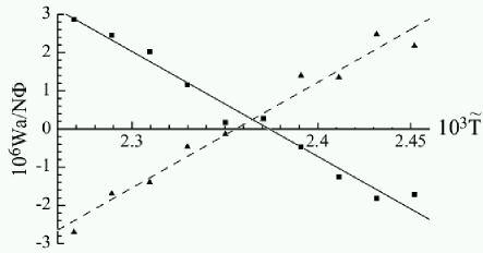
Figure 2: Simulation results for $\lambda=5,\dot{\zeta}=10^{-4}/\tau_{E}$. Solid triangles are values of $W_{bf}$, solid squares are values of $W_{fb}$. The dashed and solid lines are linear fits to the results. $\widetilde{T}_{bf}$ and $\widetilde{T}_{fb}$ are the intersections of these lines with W = 0.

We obtained results similar to those shown in Figure 2 over the entire investigated range of $\lambda$ and for three different values of $\dot{\zeta}$. Near the transition line, $W_{bf}(\lambda,\widetilde{T})$ and $W_{fb}(\lambda,\widetilde{T})$ vary linearly with $\widetilde{T}$ and have nearly opposite ($\lambda$-dependent) slopes. The scatter about linear fits to $W_{bf}(\lambda,\widetilde{T})$ and $W_{fb}(\lambda,\widetilde{T})$ is consistent with fluctuations in $W_{bf}$ and $W_{fb}$ at fixed $(\lambda,\widetilde{T})$. The intersections of these fits with $W=0$ give two estimates, $\widetilde{T}_{bf}$ and $\widetilde{T}_{fb}$, for $\widetilde{T}_{trans}$. These are obtained using data at ten evenly spaced $\widetilde{T}$ within about 5% of the transition line.

For a given system, $\widetilde{T}_{fb}$ and $\widetilde{T}_{bf}$ provide upper and lower bounds on $\widetilde{T}_{trans}$ since $W_{bf}>\Delta F>-W_{fb}$ and $(\partial{\Delta F}/\partial{\widetilde{T}})>0$. We define the fractional uncertainty due to dissipative hysteresis as

$$\delta_{hyst}=(\widetilde{T}_{fb}-\widetilde{T}_{bf})/(\widetilde{T}_{fb}+\widetilde{T}_{bf}).$$ (8)

The conditions $\delta_{hyst}\sim\dot{\zeta}$ and $<W_{cycle}>\sim\dot{\zeta}$ are equivalent due to the linear dependence of $W_{bf}$ and $W_{fb}$ on $\widetilde{T}$. Figure 3 shows the $\dot{\zeta}$-dependence of $\delta_{hyst}$ for $\lambda=4$ and $\lambda=5$. The results are consistent with our hypothesis that the energy dissipated is linear in $\dot{\zeta}$.

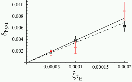
Figure 3: Strain-rate dependence of $\delta_{hyst}$. Solid circles indicate $\lambda=4$ results. Empty squares indicate $\lambda=5$ results. The solid and dashed lines are linear fits to the data. The error bars indicate statistical uncertainties. (Color online)

We identify $\widetilde{T}_{trans}=(\widetilde{T}_{bf}+\widetilde{T}_{fb})/2$ as the best estimate for the transition temperature for a given system size, system geometry, and potential cutoff radius. Table 1 shows that the fractional variation of $\widetilde{T}_{trans}$ with $\dot{\zeta}$ is much smaller than $\delta_{hyst}$ .

Table 1: Dependence of $\widetilde{T}_{trans}(\lambda)$ on dimensionless strain rate.

$\dot{\zeta}\tau_{E}$	$10^{3}\widetilde{T}_{trans}(\lambda=4)$	$10^{3}\widetilde{T}_{trans}(\lambda=5)$
$5\cdot 10^{-5}$	$1.637\pm.003$	$2.363\pm.002$
$1\cdot 10^{-4}$	$1.634\pm.004$	$2.365\pm.004$
$2\cdot 10^{-4}$	$1.633\pm.005$	$2.366\pm.005$

In the following, we present results for $|\dot{\zeta}|=10^{-4}/\tau_{E}$. Based on Table 1, for this value of $|\dot{\zeta}|$ the random and finite strain rate uncertainties in $\widetilde{T}_{trans}$ are comparable, both about 0.2%. The combined error is estimated to be less than 0.4%. The uncertainties given in subsequent tables include only statistical uncertainties from the linear fits used to calculate $\widetilde{T}_{bf}$ and $\widetilde{T}_{fb}$.

III.2 Potential cutoff dependence

We estimate the errors introduced by truncating the force at $r_{c}$ by calculating the error $\delta E(r_{c})$ in the potential energy difference. If the error in $\Delta F$ is of the same order, then the fractional error in the transition temperature is

$$\delta_{cut}\equiv\frac{\delta\widetilde{T}(r_{c})}{\widetilde{T}}\simeq\frac{1}{\widetilde{T}}\frac{\partial{\widetilde{T}}}{\partial\Delta F}\delta E(r_{c}).$$ (9)

Here $(\partial\widetilde{T}/\partial\Delta F)$ is known near the transition line from the work calculations.

The cutoff-induced error in the potential energy difference can be written in terms of the pair correlation functions $g_{fcc}(r)$ and $g_{bcc}(r)$ of the fcc and bcc crystals. For N particles

$$\delta E(r_{c})=\frac{N}{2}\int_{r_{c}}^{\infty}U(r)(g_{fcc}(r)-g_{bcc}(r))4\pi r^{2}dr/a^{3}$$ (10)

If $\Omega\equiv\textrm{max}\{|g_{fcc}(r)-g_{bcc}(r)|;r\geq r_{c}\}$, then

$$\small\frac{|\delta E(r_{c})|}{N(\Phi/a)}<\frac{\Omega}{\Phi a^{2}}\int_{r_{c}}^{\infty}U(r)2\pi r^{2}dr=\frac{2\pi\Omega(1+\lambda r_{c}/a)e^{-\lambda r_{c}/a}}{\lambda^{2}}$$ (11)

One expects $\Omega$ to be of order 1 at finite temperature.

For $\lambda$ = 3, 4, and 5, we estimated $\delta E(r_{c})$ at $\widetilde{T}\simeq\widetilde{T}_{trans}$ by calculating the pair correlation functions in large systems using large cutoff radii and long integration times. Due to the exponential falloff of U(r) and finite temperature smoothing of g(r), the infinite upper bound in Eq.  10) can be replaced by a finite value $r_{l}$ without introducing significant errors. We found $\lambda r_{l}=30a$ to be sufficiently large.

Figure 4 shows our estimate of $|\delta E(r_{c})/(N\Phi/a)|$ from Eq. (10) and the value of $|\delta E/(N\Phi/a)|$ corresponding to $\delta_{cut}=0.01$ for $\lambda=3$, the longest-range potential considered. We found that $\Omega$ decreases from 1.4 to .62 as $r_{c}$ increases from 3.5a to 6.5a. The actual error is always smaller than the bound given by $\Omega$ because $g_{fcc}-g_{bcc}$ oscillates in sign. The envelope shown corresponds to $\Omega=1/3$. Because of the sharp variation of $\delta E(r_{c})$, we use the envelope to estimate $\delta_{cut}$.

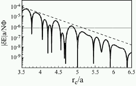
Figure 4: Determination of $r_{c}$ for $\lambda=3$. The heavy curve is our estimate of $\delta E(r_{c})$ obtained from simulations at $\widetilde{T}=8.84\cdot 10^{-3}$, with $r_{l}=10a$. The dashed line is the analytic upper bound on $\delta E(r_{c})$ from Eq.(11) with $\Omega=1/3$. The horizontal line is the value of $|\delta E|$ in Eq.(9) corresponding to $|\delta_{cut}|=0.01$.

To test Eq. (9) we calculated $\widetilde{T}_{trans}$ as a function of $r_{c}$ for $\lambda=3$. Results are shown in Table 2. The fractional changes in $\widetilde{T}_{trans}$ from $r_{c}=3.5a$ and $r_{c}=4.667a$ to $r_{c}=6.667a$ are 19% and 0.9%, respectively. Both changes are about one-fifth of the estimates for $\delta_{cut}$ from Eqs. (9,10). No statistically significant changes are expected or observed for $r_{c}\geq 5.833a$. We conclude that errors estimated from the envelopes of curves like Fig. 4 give a conservative estimate of cutoff errors.

Table 2: $\widetilde{T}_{trans}$ vs. $r_{c}$ for $\lambda=3$. $|\delta_{cut}|$ is given by Eq. 9 and the bound in Eq. 11.

$r_{c}$	$|\delta_{cut}|$	$10^{3}\widetilde{T}_{trans}$
3.5a	1.04	$1.048\pm.003$
4.667a	$0.041$	$0.871\pm.002$
5.833a	$0.0015$	$0.880\pm.002$
6.667a	$0.00014$	$0.879\pm.003$

To ensure that the fractional systematic errors were no larger than our random and rate errors, we chose $r_{c}$ slightly above the values corresponding to $|\delta_{cut}|=0.002$. For $\lambda$ = 3, 4, and 5, we used cutoff radii of 5.833a, 4.375a, and 3.5a in the simulations used to determine $\widetilde{T}_{trans}$. Smaller $r_{c}$ can be used at higher $\lambda$ both because the interactions weaken and $\widetilde{T}_{trans}/\widetilde{T}_{melt}$ increases, leading to a smaller $\Omega$. For $\lambda\geq 5$ we fixed the cutoff radius at $r_{c}=3.5a$.

III.3 System size and geometry dependence

To examine finite size effects we also considered a 432-particle system (initial state $6^{3}$ bcc unit cells). Because the corresponding fcc state has transverse length $6.73a$, the minimum image convention requires $r_{c}<3.367a$, and we used $r_{c}=3.3a$. To separate out $r_{c}$-dependence from system size dependence, we also recalculated the transition line for $N=3456$ for $5\leq\lambda\leq 8$ with $r_{c}=3.3a$.

Table 3 shows a comparison of our calculated transition temperatures. The $N=432$ values were systematically lower, but the effect was small. From theoretical considerations one expects the leading finite size corrections to $\Delta F/N$ to be proportional to $1/N$ Polson et al. (2000). This should produce a corresponding error in $\widetilde{T}_{trans}$. As shown in Table 3, the changes in $\widetilde{T}_{trans}$ from $N=432$ to $N=3456$ were all about 1%. The changes in $\widetilde{T}_{trans}$ from $N=3456$ to $N=\infty$ for this system geometry should be about 8 times smaller.

Table 3: Dependence of $\widetilde{T}_{trans}$ on N.

$\lambda$	$10^{3}\widetilde{T}_{trans}(N=432)$	$10^{3}\widetilde{T}_{trans}(N=3456)$
5	$2.350\pm.009$	$2.362\pm.004$
6	$2.985\pm.011$	$3.021\pm.003$
7	$3.562\pm.009$	$3.593\pm.005$
8	$4.064\pm.008$	$4.087\pm.005$

Another test indicates that finite size effects are larger than the above estimate. The geometry was changed so that the fcc state has equal cell edges and the bcc state has $L_{x}=L_{y}=\sqrt{2}L_{z}$. These simulations contained $10^{3}$ fcc unit cells (4000 particles) with the $<100>$ directions parallel to the simulation cell edges. After Bain transformation, the bcc state has two $<110>$ directions parallel to the simulation cell edges. As shown in Table 4, the values of $\widetilde{T}_{trans}$ obtained for both $\lambda=4$ and $\lambda=7$ were 0.6% lower than those obtained with the standard system geometry . Other simulations verified that this was due solely to the change in boundary conditions. We conclude that our dominant source of uncertainty is finite size and is less than 1%.

Table 4: Dependence of $\widetilde{T}_{trans}$ on system geometry.

$\lambda$	$10^{3}\widetilde{T}_{trans}(N=3456)$	$10^{3}\widetilde{T}_{trans}(N=4000)$
4	$1.634\pm.004$	$1.625\pm.004$
7	$3.592\pm.004$	$3.570\pm.004$

We attribute the observed sensitivity to geometry to the change in allowed low frequency modes. These modes play a disproportionate role in determining the entropy in lattice dynamics calculations Robbins et al. (1990) and drive the fcc$\to$bcc transition with increasing temperature Robbins et al. (1988). Since the shear velocity is highly anisotropic in the bcc phase, changing the boundaries affects the sampling of these low frequency modes and thus $\Delta F$.

III.4 Transition line

Table 5 shows our calculated $\widetilde{T}_{trans}(\lambda)$ with statistical uncertainties. As described above, the combined systematic errors due to finite strain rate, system size, and potential cutoff are estimated to be less than 1%. Results of a cubic polynomial fit to the data are also given:

$$\begin{array}[]{lcl}10^{4}\widetilde{T}_{trans}^{fit}(\lambda)&=&6.46678(\lambda-\lambda_{0})+0.43001(\lambda-\lambda_{0})^{2}\\ &&-0.06806(\lambda-\lambda_{0})^{3},\end{array}$$ (12)

where $\lambda_{0}=1.718$ is the zero-temperature transition point obtained from lattice statics calculations e Silva and Mockross (1980). Lower-order polynomials fail to adequately fit the data within our uncertainties.

Table 5: Calculated and fit values of $\widetilde{T}_{trans}$. Only statistical uncertainties are quoted.

$\lambda$	$10^{3}\widetilde{T}_{trans}$	$10^{3}\widetilde{T}^{fit}_{trans}$
3	$0.880\pm.002$	0.885
4	$1.634\pm.004$	1.619
5	$2.365\pm.004$	2.345
6	$3.017\pm.004$	3.023
7	$3.592\pm.004$	3.613
8	$4.085\pm.004$	4.072

Figure 5 shows the polynomial fit and two previously published solid-fluid coexistence lines Stevens and Robbins (1993); Hamaguchi et al. (1997). The intersections of these lines give estimated values of the bcc-fcc-fluid triple point. Using results from Ref. Stevens and Robbins (1993) we find $(\lambda_{tp}=7.45,\widetilde{T}_{tp}=0.00384)$. Those from Ref. Hamaguchi et al. (1997) yield $(\lambda_{tp}=7.84,\widetilde{T}_{tp}=0.00401)$.

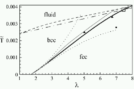
Figure 5: Phase diagram of Yukawa systems. The heavy line is our cubic polynomial fit for the bcc-fcc transition line. The light solid line is the fcc-bcc transition line from Ref. Hamaguchi et al. (1997). The low and high dotted lines are respectively the lattice dynamics and molecular dynamics bcc-fcc transition lines from Ref. Robbins et al. (1988). The triangles are a bcc-fcc coexistence point and triple point from Ref. Dupont et al. (1993), and the solid square is a bcc-fcc transition point from Ref. Miller and Reinhardt (2000). The dashed and dash-dotted lines are the melting lines from Ref. Stevens and Robbins (1993) and Ref. Hamaguchi et al. (1997). The empty squares denote our estimates for the bcc-fcc-fluid triple point.

If we assume that the parameters $\kappa$ and $\Phi$ are density-independent, we can calculate the width of the bcc-fcc coexistence region from the pressures and bulk moduli of the two phases on the line where $\Delta F=0$. The bcc pressure is larger than the fcc pressure by only about 0.04% for $\lambda=4$, and by 0.65% for $\lambda=7$. This results in a higher density in the fcc phase at coexistence, but only by about 0.015% at $\lambda=4$ and 0.2% at $\lambda=7$. The corresponding changes in $\lambda$ and $\widetilde{T}$ are much smaller than the uncertainties in our calculated transition line. The coexistence region in experimental systems may be much larger due to variations in $\kappa$ and $\Phi$ with density Schope et al. (1998); et.al (2003). As noted above, these variations are system specific and a more complete treatment is beyond the scope of this paper.

III.5 Anharmonic effects

The dotted line in Figure 5 shows lattice dynamics results for the bcc-fcc transition line Robbins et al. (1988). In this approximation the energy and entropy differences, $\Delta E_{LD}$ and $\Delta S_{LD}$, are independent of T. The fcc-bcc transition line is given by $T_{LD}=\Delta E_{LD}/\Delta S_{LD}$. The resulting curve lies below $\widetilde{T}_{trans}$, indicating that the fcc phase is stabilized by anharmonic effects Robbins et al. (1988); Hamaguchi et al. (1997). This implies that the anharmonic component of the free energy difference,

$$\Delta F_{an}\equiv\Delta E_{an}-T\Delta S_{an}=\Delta F-\Delta F_{LD},$$ (13)

is negative on the transition line. The relative signs and magnitudes of $\Delta E_{an}$ and $\Delta S_{an}$ may be calculated by comparing our accurate measurements of free and total energy differences with the lattice-dynamics results.

Table 6 shows results for anharmonic contributions to the free and total energy differences on the fit transition line . The values of $\Delta F_{an}$ are known from the work calculations, while the values of $\Delta E_{an}$ were found from separate equilibrium simulations. The anharmonic corrections to the total energy favor the bcc phase for all $\lambda$, i.e., $E_{fcc}-E_{bcc}$ on the transition line has increased relative to its zero-temperature value. The anharmonic contributions to the free energy difference, however, are larger in magnitude and opposite in sign, implying that anharmonic entropic contributions to $\Delta F$ favor the fcc phase at all $\lambda$ and overwhelm energetic contributions.

Table 6: Anharmonic free and total energy differences evaluated at $\widetilde{T}^{fit}_{trans}(\lambda)$.

$\lambda$	$10^{2}\Delta F_{an}/Nk_{B}T$	$10^{2}\Delta E_{an}/Nk_{B}T$
3	$-0.58\pm 0.1$	$0.42\pm 0.33$
4	$-1.07\pm.12$	$1.0\pm.4$
5	$-1.92\pm.15$	$1.2\pm.4$
6	$-3.03\pm.17$	$2.4\pm.4$
7	$-4.33\pm.21$	$2.2\pm.4$

In lattice calculations the larger entropy of the bcc phase comes mainly from the lower frequency of its shear modes. Some of these modes have negative energy for $\lambda>7.67$, causing the bcc phase to become linearly unstable at low temperatures Robbins et al. (1988). It is interesting that the onset of this low temperature instability is close to $\lambda_{tp}$. However, we have performed runs near the melting line for $\lambda$ as large as 10 and find that the bcc phase remains metastable. This implies that anharmonic effects have increased the frequency of long wavelength shear modes, providing an explanation for the decreased entropy advantage of the bcc phase.

IV Comparison to Previous Results

Miller and Reinhardt were the first authors to use Bain deformation paths to obtain bounds on $\Delta F$ for Yukawa systems Miller and Reinhardt (2000). They calculated the work by integrating the change in the Hamiltonian rather than from the stresses and strains. The large discrepancy between their $\lambda=7$ transition temperature and our result is likely due to their extremely small system size $(N=108)$, which was just used to illustrate their method.

The earliest MD calculations Kremer et al. (1986); Robbins et al. (1988) of the transition line also deviate substantially from ours, particularly at large $\lambda$. The line shown in Figure 5 is a fit between points where the fcc and bcc phases were found to be stable. The gap between points was about 20% and the final shape was strongly influenced by a bcc-stable point above the melting line. Other points where the bcc phase was stable lie close to our $\widetilde{T}_{trans}$ but are shifted up due to the smaller $r_{c}$ used.

Our transition line is in qualitative agreement with more recent MD and Monte Carlo results Hamaguchi et al. (1997); Dupont et al. (1993). Dupont et. al. calculated a fcc-bcc coexistence point and the fcc-bcc-fluid triple point using small systems $(N\simeq 250)$. Although their triple point $(\lambda_{tp}=6.75,\widetilde{T}_{tp}=0.0034)$ lies well below ours $(\lambda_{tp}=7.7\pm 0.3,\widetilde{T}_{tp}=0.0039\pm 0.0001)$, it lies only about 2% below our fcc-bcc transition line, and well below recently published melting lines Stevens and Robbins (1993); Hamaguchi et al. (1997).

Hamaguchi, Farouki, and Dubin also obtain a lower triple point $(\lambda_{tp}=6.90,\widetilde{T}_{tp}=0.0038)$ because their bcc-fcc transition temperatures are systematically (6-10%) higher than ours Hamaguchi et al. (1997). One possible explanation is that their equilibration times were too short. They used the $\lambda$-independent time unit $\tau=\sqrt{3}\omega_{p}^{-1}$, where $\omega_{p}=\sqrt{4\pi n\Phi/m}$ is the plasma frequency. Starting with perfect bcc and fcc lattices as their initial conditions, they equilibrated their systems for a maximum of 300$\tau$ before beginning their free energy measurements. This corresponds to about 27$\tau_{E}$ for $\lambda=3$ and only 4$\tau_{E}$ for $\lambda=8$. Since the latter is only about four times the velocity autocorrelation time, and comparable to the time for sound to propagate across their simulation cells, it is doubtful that their systems had equilibrated sufficiently at high $\lambda$. Too short an equilibration time could cause overestimation of the stability of the phase with lower entropy, the fcc phase, which is consistent with their findings.

Vaulina and colleagues have proposed phenomenological criteria for the bcc-fcc transition Vaulina et al. (2002). They assume that $\kappa^{-1}$ is an effective hard-sphere radius and predict that the value of the rms displacement at the fcc transition, $\Delta_{trans}$, satisfies

$$2(1-\pi\sqrt{2}/6)^{-1/3}\Delta_{trans}=R_{WS}-\kappa^{-1}$$ (14)

where $R_{WS}=(4\pi/3)^{-1/3}a$ is the Wigner-Seitz radius. They then use an approximate formula for the effective frequency in an Einstein-like model to determine $\Delta$ for the fcc and bcc structures. These values of $\Delta$ give two predictions for the transition line. As shown in Figure 6, their predictions are qualitatively correct but lie roughly 10-40% above our $\widetilde{T}_{trans}$.

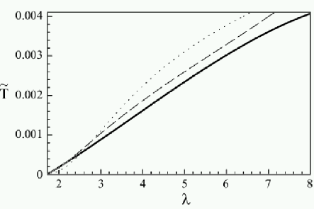
Figure 6: Comparison of transition line to analytic estimates. The heavy line is our $\widetilde{T}^{fit}_{trans}(\lambda)$. The dashed and dotted lines are the analytic estimates for the bcc$\to$fcc and fcc$\to$bcc transitions from Ref. Vaulina et al. (2002).

The discrepancy in Fig. 6 could be due to a failure either of Eq. (14) or of the approximations used to find $\Delta$. To test this we performed equilibrium simulations at $\widetilde{T}^{fit}_{trans}$ in both bcc $(N=3456)$ and fcc $(N=4000)$ systems. Our results for the rms displacements, $\Delta_{fcc}$ and $\Delta_{bcc}$, are compared to the predictions of Eq. (14) in Table 7. The rms displacements for the fcc structure lie quite close to the prediction for small $\lambda$, and about 13% above it at $\lambda=7$. Finite size effects decrease $\Delta_{fcc}$ relative to the N = $\infty$ value Robbins et al. (1990) . These results indicate that most of the error in Vaulina et. al.’s transition lines comes from substantial underestimation of the rms displacements. They calculate $\Delta$ in the harmonic approximation, and anharmonic corrections increase $\Delta$ for these $\lambda$ Robbins et al. (1988). Note that the measured bcc displacements in Table VI are larger due to the bcc lattice’s softer shear modes Robbins et al. (1988).

Table 7: Rms displacements at $\widetilde{T}^{fit}_{trans}(\lambda)$. $\Delta_{trans}$ is the prediction from Eq.14, while $\Delta_{fcc}$ and $\Delta_{bcc}$ are results from equilibrium MD simulations.

$\lambda$	$\Delta_{trans}$	$\Delta_{fcc}$	$\Delta_{bcc}$
3	0.0915	0.089	0.096
4	0.1181	0.118	0.128
5	0.1341	0.140	0.154
6	0.1447	0.159	0.177
7	0.1522	0.171	0.192

V Summary and Conclusions

We calculated the bcc-fcc coexistence line of Yukawa systems to an uncertainty of approximately 1% through integration of the mechanical work along Bain transformation paths. The range of bcc stability was found to be slightly greater than that found in previous comprehensive studies Robbins et al. (1988); Dupont et al. (1993); Hamaguchi et al. (1997), and the triple point shown to lie at higher inverse screening length. The large changes in $\widetilde{T}_{trans}$ with $r_{c}$ for small $\lambda$ indicate that the relative stability of fcc and bcc phases depends sensitively on long-range correlations, and calls into question the use of local nearest-neighbor arguments to calculate the transition line. Nevertheless, we found that one such phenomenological criterion Vaulina et al. (2002), derived from the idea that the fcc phase is stable when interparticle interactions are hard-sphere-like Hoover and Ree (1968), predicts the transition line remarkably well when combined with MD results for the mean-squared displacement.

Comparison with lattice-dynamics results shows that anharmonic terms in the total energy favor the bcc phase for all $\lambda$, but that these corrections are overbalanced by anharmonic contributions to the entropy. The change in entropy appears to reflect an increase in the frequency of long-wavelength shear modes in the bcc phase. This increase also stabilizes the bcc phase against a linear shear instability observed for $\lambda>7.67$ at low $\widetilde{T}$.

We found that shifts in the transition line due to finite size effects are less than 1% if N$\sim$3000-4000, but that the presence of long-range order at temperatures near the transition line in weakly screened systems requires a cutoff radius larger than that used in some previous studies Kremer et al. (1986); Robbins et al. (1988). Accurate simulations of weakly screened ($\lambda<3$) systems in this temperature range require either larger system sizes or an Ewald-like summation over periodic images Hamaguchi et al. (1997). However, we have also shown that a reasonably small potential cutoff need not introduce large errors in a transition line calculation in the moderate-screening regime, provided the cutoff is chosen with some care.

It is known that the phase behavior of real systems such as charge-stabilized colloidal suspensions is not fully described by pointlike Yukawa interactions. Recent simulations of charged macroions in a dynamic neutralizing background have shown that the repulsive interactions between macroions are truncated by many-body effects, destabilizing the crystalline phases in the weak screening limit Dobnikar et al. (2003a, b); Hynninen and Dijkstra (2003a). Independently, hard-core repulsions significantly alter the phase diagram when the volume fraction is more than a few percent Meijer and Azhar (1997); Azhar et al. (2000); Hynninen and Dijkstra (2003b). However, we hope that our high-precision calculation of the point Yukawa fcc-bcc transition line may serve as a benchmark for further studies of more sophisticated models.

VI Acknowledgements

The simulations in this paper were carried out using the LAMMPS molecular dynamics software. Support from NSF Grant DMR-0083286 is gratefully acknowledged.

References

- Ashcroft and Mermin (1976) N. W. Ashcroft and N. D. Mermin, Solid State Physics (Saunders College Publishing, 1976).
- Whipple et al. (1985) E. C. Whipple, T. Northrop, and D. Mendis, J. Geophys. Res. 90, 7405 (1985).
- Hamaguchi and Farouki (1994) S. Hamaguchi and R. T. Farouki, J. Chem. Phys. 101, 9876 (1994).
- Rosenfeld (1994) Y. Rosenfeld, Phys. Rev. E 49, 4425 (1994).
- Verwey and Overbeek (1948) E. Verwey and J. T. G. Overbeek, Theory of the Stability of Lyophilic Colloids (Elsevier, 1948).
- Alexander et al. (1984) S. Alexander, P. Chaikin, P. Grant, G. J. Morales, and P. Pincus, J. Chem. Phys. 80, 5776 (1984).
- Stevens et al. (1996) M. J. Stevens, M. L. Falk, and M. O. Robbins, J. Chem. Phys. 104, 5209 (1996).
- Palberg et al. (1995) T. Palberg, W. Monch, F. Bitzer, R. Piazza, and T. Bellini, Phys. Rev. Lett. 74, 4555 (1995).
- Shih and Stroud (1983) W.-H. Shih and D. Stroud, J. Chem. Phys. 79, 6254 (1983).
- Vaulina et al. (2002) O. S. Vaulina, S. V. Vladimirov, O. F. Petrov, and V. E. Fortov, Phys. Rev. Lett. 88, article 245002 (2002).
- Hone et al. (1983) D. Hone, S. Alexander, P. Chaikin, and P. Pincus, J. Chem. Phys. 79, 1474 (1983).
- Tejero et al. (1992) C. F. Tejero, J. F. Lutsko, J. L. Colot, and M. Baus, Phys. Rev. A 46, 3373 (1992).
- Vaulina (2002) O. S. Vaulina, J. Exp. Theor. Phys. 94, 26 (2002).
- Rosenberg and Thirumalai (1987) R. O. Rosenberg and D. Thirumalai, Phys. Rev. A 36, 5690 (1987).
- Meijer and Frenkel (1991) E. J. Meijer and D. Frenkel, J. Chem. Phys. 94, 2269 (1991).
- Zahorchak et al. (1992) J. C. Zahorchak, R. Kesavamoorthy, R. D. Coalson, and S. A. Asher, J. Chem. Phys. 96, 6873 (1992).
- Stevens and Robbins (1993) M. J. Stevens and M. O. Robbins, J. Chem. Phys. 98, 2319 (1993).
- Farouki and Hamaguchi (1994) R. T. Farouki and S. Hamaguchi, J. Chem. Phys. 101, 9885 (1994).
- Hamaguchi et al. (1996) S. Hamaguchi, R. T. Farouki, and D. H. E. Dubin, J. Chem. Phys. 105, 7641 (1996).
- Kremer et al. (1986) K. Kremer, M. O. Robbins, and G. S. Grest, Phys. Rev. Lett. 57, 2694 (1986).
- Robbins et al. (1988) M. O. Robbins, K. Kremer, and G. S. Grest, J. Chem. Phys. 88, 3286 (1988).
- Dupont et al. (1993) G. Dupont, S. Moulinasse, J. P. Ryckaert, and M. Baus, Mol. Phys. 79, 453 (1993).
- Hamaguchi et al. (1997) S. Hamaguchi, R. T. Farouki, and D. H. E. Dubin, Phys. Rev. E 56, 4671 (1997).
- Miller and Reinhardt (2000) M. A. Miller and W. P. Reinhardt, J. Chem. Phys. 113, 7035 (2000).
- Chu and I (1994) J. H. Chu and L. I, Phys. Rev. Lett. 72, 4009 (1994).
- et.al (2003) A. P. Nefedov et. al., New J. Phys. 5, article 33 (2003).
- Monovoukas and Gast (1989) Y. Monovoukas and A. P. Gast, J. Colloid Interface Sci. 128, 533 (1989).
- Sirota et al. (1989) E. B. Sirota, H. D. Ou-Yang, S. K. Sinha, P. M. Chaikin, J. D. Axe, and Y. Fujii, Phys. Rev. Lett. 62, 1524 (1989).
- Schope et al. (1998) H. Schope, T. Decker, and T. Palberg., J. Chem. Phys. 109, 10068 (1998).
- Straatsma et al. (1986) T. P. Straatsma, H. J. C. Berendsen, and J. P. M. Postma, J. Chem. Phys. 85, 6720 (1986).
- Reinhardt and Hunter (1992) W. P. Reinhardt and J. E. Hunter, J. Chem. Phys. 97, 1599 (1992).
- Hunter et al. (1993) J. E. Hunter, W. P. Reinhardt, and T. F. Davis, J. Chem. Phys. 99, 6856 (1993).
- Reif (1965) F. Reif, Fundamentals of Statistical and Thermal Physics (McGraw Hill, 1965).
- Milstein et al. (1994) F. Milstein, H. E. Fang, and J. Marschall, Philos. Mag. 70, 621 (1994).
- Hoover et al. (1980) W. G. Hoover, D. J. Evans, R. B. Hickman, A. J. C. Ladd, W. T. Ashurst, and B. Moran, Phys. Rev. A 22, 1690 (1980).
- Swope et al. (1982) W. C. Swope, H. C. Andersen, P. H. Berens, and K. Wilson, J. Chem. Phys. 76, 637 (1982).
- Schneider and Stoll (1978) T. Schneider and E. Stoll, Phys. Rev. B 17, 1302 (1978).
- Allen and Tildesly (1987) M. P. Allen and D. J. Tildesly, Computer Simulation of Liquids (Clarendon Press, 1987).
- Jarzynski (1997) C. Jarzynski, Phys. Rev. Lett. 78, 2690 (1997).
- Larson (1999) R. G. Larson, The Structure and Rheology of Complex Fluids (Oxford University Press, 1999).
- Polson et al. (2000) J. M. Polson, E. Trizac, S. Pronk, and D. Frenkel, J. Chem. Phys. 112, 5339 (2000).
- Robbins et al. (1990) M. O. Robbins, G. S. Grest, and K. Kremer, Phys. Rev. B 42, 5579 (1990).
- e Silva and Mockross (1980) J. Medeiros e Silva and B. J. Mockross, Phys. Rev. B 21, 2972 (1980).
- Hoover and Ree (1968) W. G. Hoover and F. H. Ree, J. Chem. Phys. 49, 3609 (1968).
- Dobnikar et al. (2003a) J. Dobnikar, R. Rzehak, and H. H. von Grunberg, Europhys. Lett. 61, 695 (2003a).
- Dobnikar et al. (2003b) J. Dobnikar, Y. Chen, R. Rzehak, and H. H. von Grunberg, J. Chem. Phys. 119, 4971 (2003b).
- Hynninen and Dijkstra (2003a) A. P. Hynninen and M. Dijkstra, J. Phys. Cond. Matt. 15, 3557 (2003a).
- Meijer and Azhar (1997) E. J. Meijer and F. E. Azhar, J. Chem. Phys. 106, 4678 (1997).
- Hynninen and Dijkstra (2003b) A. P. Hynninen and M. Dijkstra, Phys. Rev. E 68, 21407 (2003b).
- Azhar et al. (2000) F. E. Azhar, M. Baus, J. Ryckaert, and E. Meijer, J. Chem. Phys. 112, 5121 (2000).