Collective Modes of $\nu=2$ Quantum Hall Bilayers in Tilted Magnetic Field

Abstract

We use time-dependent Hartree Fock approximation to study the collective mode spectra of $\nu=2$ quantum Hall bilayers in tilted magnetic field allowing for charge imbalance as well as tunneling between the two layers. In a previous companion paper to this work, we studied the zero temperature global phase diagram of this system which was found to include a symmetric and ferromagnetic phases as well as a first order transition between two canted phases with spontaneously broken $U(1)$ symmetry. We further found that this first order transition line ends in a quantum critical point within the canted region. In the current work, we study the excitation spectra of all of these phases and pay particular attention to the behavior of the collective modes near the phase transitions. We find, most interestingly, that the first order transition between the two canted phases is signaled by a near softening of a magnetoroton minimum. Many of the collective mode features explored here should be accessible experimentally in light scattering experiments.

I Introduction

Scattering experiments have provided extremely powerful and important probes of two dimensional electron systemsSarma and Pinczuk (1997). A particularly nice application of light scattering was a recent set experimentsPellegrini et al. (1997, 1998) on quantum Hall bilayers with equal densities in each layer. An apparent mode softening at total filling fraction $\nu=2$ was identified with the existence of a Goldstone mode which fit well with prior predictions of a novel canted phase in these bilayer systemsZheng et al. (1997); Sarma et al. (1998). The experiments were conducted using the tilted-field technique for sweeping across a wide range of Zeeman energies in situ. Interestingly, tilted magnetic fields also have a non-trivial effect on interlayer tunneling. Furthermore, as noted first by Burkov and MacDonald Burkov and MacDonald (2002), in $\nu=2$ bilayer systems with a charge-imbalance between the layers, tilting the magnetic field can induce a new first order quantum phase transition embedded in the canted phase. As shown by the current authors in the preceding companion paper to this workLopatnikova et al. (2003), the first order transition separates two phases with the same symmetry which are topologically connected in the phase diagram. Similar to a liquid-gas transition, the first order phase transition line terminates at a quantum critical point. In our preceding paperLopatnikova et al. (2003) we discussed the phases and phase transitions of $\nu=2$ in detail, accounting for both charge imbalance and in-plane magnetic field. The purpose of the present work is to examine the excitation spectra of these different phases in order to make connection with possible future experiments. Particular attention will be paid to the evolution of the collective-mode dispersions across the new first-order transition induced by the tilted magnetic field.

Bilayer quantum Hall systems in general have been the focus of a great deal of recent studydassarma2 . The already rich physics of quantum Hall effects is further enhanced in bilayers by the added degree of freedom. The most studied of the bilayer quantum Hall state is certainly the $\nu=1$ statedassarma2 . At $\nu=1$ the spin degrees of freedom are effectively frozen out, and all the interesting physics occurs in the isospin (layer degrees of freedom). In contrast, for $\nu=2$ systems, not only the layer but also the spin degrees of freedom are important. Indeed, in several of the phases of $\nu=2$, the spin and isospin degrees of freedom are actually entangled.

In perpendicular magnetic field, $\nu=2$ bilayers exhibit the many-body canted phase at finite tunnelingZheng et al. (1997). This phase is a spontaneously-broken $U(1)$ symmetry phase, despite the finite tunneling. This is in marked contrast with the $\nu=1$ bilayers, in which a $U(1)$ symmetric phase is possible only in the absence of tunneling. Things change when a finite voltage bias is added: In this case, $\nu=2$ bilayers can exhibit a many-body phase in the absence of tunneling. This phase is somewhat akin to the many-body phase of $\nu=1$ bilayers, as was pointed out by MacDonald, Rajaraman, and JungwirthMacDonald et al. (1999). These authors therefore mused that, in the presence of a finite in-plane magnetic field component, $\nu=2$ bilayers may also undergo a commensurate incommensurate transition.

Burkov and MacDonaldBurkov and MacDonald (2002) explored this possibility. Indeed, they found that charge-unbalanced $\nu=2$ bilayers can undergo a phase transition driven by the in-plane field component. However, the phase transition was between two commensurate phases, instead of a between a commensurate and an incommensurate phase. One of the commensurate phases was akin to the commensurate phase of the $\nu=1$ bilayers – the isospin component followed the magnetic field. The other commensurate phase however, was more peculiar: in this phase, both isospin and spin components were commensurate with the in-plane field! In our previous publication, we attempted to understand the physics behind this spin-commensuration. We explored the phase transition further, and found that it terminates at a critical point within the canted phase (See Fig. 1).

Figure 1: Global phase diagram of charge-unbalanced $\nu=2$ bilayers in tilted magnetic field. The phase diagram is calculated for bare tunneling gap $\Delta_{SAS}^{0}=0.06e^{2}/(\varepsilon l)$, Zeeman energy $\Delta_{Z}^{0}=0.01e^{2}/(\varepsilon l)$, and the distance between the layers $d=l$. The axes are the amplitude of the in-plane field wavevector: $\vec{Q}_{||}=\frac{\hat{z}\times\vec{B}_{||}}{(B_{\perp}l^{2}/d)}$ and the external bias voltage $\Delta_{V}$. This choice of axes is particularly suitable, since current experimental techniques allow to vary the bias voltage and the in-plane field in situ over a wide range of values. $SC$ is the spin-singlet commensurate phase, $C1$ is the simple, isospin-commensurate phase, $C2$ is the spin-isospin commensurate phase. Solid lines represent the second-order quantum phase transitions, dashed line — the novel first-order $C1$–$C2$ transition.

As mentioned above, one way of experimentally distinguishing between the many phases of the $\nu=2$ bilayers is to probe the collective excitations Pellegrini et al. (1997, 1998). In this paper we therefore set out to explore this phase transition further by finding the collective modes. The many-body phases ($C1$, and $C2$ as well as $I$ which occurs in the absence of tunneling) of the $\nu=2$ bilayers are characterized by spontaneously broken symmetries, which result in the formation of low-energy Goldstone modes. In fact, the first theoretical and experimental evidence of the canted phase in charge-balanced $\nu=2$ bilayers was obtained by observing a softening spin-density mode in time-dependent Hartree-Fock (TDHF) analysis Zheng et al. (1997) and in inelastic light-scattering experiments Pellegrini et al. (1997, 1998).

More generally, the TDHF approximation allows one to predict the response of the system to any one of a number of possible experimental probes Kallin and Halperin (1984); Côté and MacDonald (1991). A general perturbation can be introduced into the system by the addition of a small time-dependent term, $\delta H$:

$$\delta H=\sum_{\mu\sigma\nu\sigma^{\prime}}\int\frac{d\omega}{2\pi}\int\frac{d^{2}k}{2\pi}\,\,\,\Phi_{\mu\sigma,\nu\sigma^{\prime}}({\bf k},\omega)e^{-i\omega t}\,\,\rho_{\mu\sigma,\nu\sigma^{\prime}}^{\dagger}({\bf k},\omega)$$ (1)

to the total Hamiltonian (Eq. (13)). The operators $\rho_{\mu\sigma,\nu\sigma^{\prime}}$ are the density operators

$$\rho_{\mu\sigma,\nu\sigma^{\prime}}({\bf k},0)=\frac{1}{g}\sum_{X}e^{-ik_{x}X-ik_{x}k_{y}l^{2}/2}c^{{\dagger}}_{\mu\sigma,X}c_{\nu\sigma^{\prime},X+k_{y}l^{2}},$$ (2)

(where $g$ is the Landau level degeneracy) whose time-evolution can be obtained using the Heisenberg equation of motion (Eq. (III)); the external time-dependent field $\Phi_{\mu\sigma,\nu\sigma^{\prime}}({\bf k},\omega)$ in Eq. (1) must turn into its complex conjugate when $\mu\sigma\leftrightarrow\nu\sigma^{\prime}$ and ${\bf k},\omega\leftrightarrow-{\bf k},-\omega$ so that the Hamiltonian remains Hermitian. Different experimental probes will couple to different combinations of the density matrix $\rho_{\mu\sigma,\nu\sigma^{\prime}}({\bf k})$. For example, a surface acoustic wave experiment might couple to the total charge density $\sum_{\nu\sigma}\rho_{\nu\sigma,\nu\sigma}$, whereas certain spin-polarized light scattering experiments might couple to the spin-flip-density $\sum_{\nu}\rho_{\nu\uparrow,\nu\downarrow}$.

If the perturbing external field $\Phi_{\mu\sigma,\nu\sigma^{\prime}}({\bf k},\omega)$ is small, one can assume that the response of the system to it is linear:

$$\langle\delta\rho_{\mu^{\prime}s,\nu^{\prime}s^{\prime}}({\bf k},\omega)\rangle=\chi^{\mbox{\small ret}}_{\mu^{\prime}s,\nu^{\prime}s^{\prime},\mu\sigma,\nu\sigma^{\prime}}({\bf k},\omega)\,\,\Phi_{\mu\sigma,\nu\sigma^{\prime}}({\bf k},\omega).$$ (3)

The proportionality coefficient between the change in the density expectation value as a result of the perturbation, $\langle\delta\rho_{\mu^{\prime}s,\nu^{\prime}s^{\prime}}({\bf k},\omega)\rangle$ and the perturbing field, $\Phi_{\mu\sigma,\nu\sigma^{\prime}}({\bf k},\omega)$, is the density response function that can be obtained in the TDHF approximation. The presence of a pole at a particular frequency and wavevector indicates resonant response (i.e. the presence of a collective mode).

We therefore start the derivation of the collective-mode dispersion of the $\nu=2$ bilayers by obtaining general expressions for the density response function. First, in Section II we review the unrestricted Hartree-Fock approximation through which the ground states of the $\nu=2$ bilayers were obtained in our previous companion paperLopatnikova et al. (2003). We then continue in Section III to derive the TDHF approximation Kallin and Halperin (1984); Côté et al. (1995); Demler et al. (2002) which is tailored to match the unrestricted Hartree-Fock of our prior study, and results in a general matrix equation for the density response function.

In Sections IV and V, collective modes of the charge-unbalanced $\nu=2$ bilayers in perpendicular field are obtained (collective modes in charge-balanced $\nu=2$ bilayers were discussed in Ref. Zheng et al. (1997) and Sarma et al. (1998)). In Section IV, the collective-mode dispersions (i.e. the poles of the density response function) of the charge-unbalanced $\nu=2$ bilayers with no interlayer tunneling are obtained in closed form. The symmetry properties that simplify the (complicated) general equations for the density response function are discussed. In Section V, the collective-mode dispersions of the charge-unbalanced $\nu=2$ bilayers in the presence of a small amount of interlayer tunneling are obtained numerically and compared to the collective-mode dispersions of the system without tunneling (Figs. 2–4).

Section VI presents our main result: the collective-mode dispersions of the $\nu=2$ bilayer systems in tilted magnetic field. A set of collective-mode dispersion curves calculated as the tilt-angle is increased and the system undergoes the $C1$–$C2$ transition is exhibited in Fig. 5. Figure 6 shows the dispersion curves of the $\nu=2$ bilayers at the critical end-point. A dramatic softening of the Goldstone mode at this point is observed.

II “Unrestricted” Hartree-Fock Approximation: An Overview

We review here the “unrestricted” Hatree-Fock first discussed previously in Refs. Burkov and MacDonald, 2002 and Lopatnikova et al., 2003. Our system consists of a disorderless zero temperature bilayer quantum Hall system with tunneling between the layers and both perpendicular and in-plane magnetic fields. Three terms of the Hamiltonian — $H_{Z}$, the Zeeman energy, $H_{V}$ the bias voltage between layers, and $H_{t}$ the tunneling — couple to single electrons and comprise the non-interacting part of the Hamiltonian

$$H_{0} = H_{Z}+H_{V}+H_{T}$$ (4)

$$= -\sum_{X}\mbox{\Large{[}}\Delta_{Z}S_{X}^{z}+\Delta_{V}I^{z}_{X}+$$

$$+\frac{\Delta_{SAS}}{2}(e^{iQ_{||}X}I^{+}_{X}+e^{-iQ_{||}X}I^{-}_{X})\mbox{\Large{]}}.$$

where $\vec{S}$ and $\vec{I}$ are the spin and isospin operators

$$\vec{S}_{X} = \frac{1}{2}\sum_{\mu\,ss^{\prime}}c^{{\dagger}}_{\mu s\,X}\vec{\sigma}_{ss^{\prime}}c_{\mu s^{\prime}\,X}^{\phantom{\dagger}}$$ (5)

$$\vec{I}_{X} = \frac{1}{2}\sum_{s\,\mu\nu}c^{{\dagger}}_{\mu s\,X}\vec{\tau}_{\mu\nu}c_{\nu s\,X}^{\phantom{\dagger}},$$ (6)

where $\vec{\sigma}$ and $\vec{\tau}$ are sets of Pauli matrices. Here, the subscript $X$ represents the momentum index of the electron state in Landau gauge, and the subscript $s$ takes on the values $+1$ and $-1$ corresponding to spin up and spin down whereas $\mu$ and $\nu$ take on the values $+1$ and $-1$ corresponding to different layer index (up and down “isospin”).

The Coulomb interactions between the electrons are taken into account by an additional term

$$H_{I}=\frac{1}{2\Omega}\sum_{\begin{array}[]{c}\mbox{\small$X_{1}X_{2}$}\\ \mbox{\small$\nu_{1},\nu_{2}$}\\ \mbox{\small$\sigma_{1},\sigma_{2}$}\end{array}}\sum_{\bf q}e^{iq_{x}(X_{1}-X_{2})}e^{-q^{2}l^{2}/2}V_{\mu_{1}\mu_{2}}(q)\times$$ (10)

$$\mbox{\hskip 20.0pt}\times c^{{\dagger}}_{\mu_{1}\sigma_{1}\,X_{1}+q_{y}l^{2}}c^{{\dagger}}_{\mu_{2}\sigma_{2}\,X_{2}}c_{\mu_{2}\sigma_{2}\,X_{2}+q_{y}l^{2}}^{\phantom{\dagger}}c_{\mu_{1}\sigma_{1}\,X_{1}}^{\phantom{\dagger}}.$$ (11)

where intra- and interlayer Coulomb interactions are

$$V_{RR}(q)=\frac{2\pi e^{2}}{\varepsilon q},\ \ V_{RL}(q)=\frac{2\pi e^{2}}{\varepsilon q}e^{-dq},$$ (12)

respectively, $d$ is the distance between the layers, and $\Omega$ is the area of the sample. The total Hamiltonian is therefore simply

$$H=H_{0}+H_{I}.$$ (13)

The Coulomb-interacting Hamiltonian in Eq. (13) is not tractable exactly, and we solve it using the Hartree-Fock approximation. In the usual manner, we assume that the many-body ground state, $|G\rangle$, is a Slater determinant of single-particle states and perform a functional minimization of the expectation value $\langle G|H|G\rangle$ with respect to these single-particle states. As was described in Refs. Burkov and MacDonald, 2002 and Lopatnikova et al., 2003, under the assumption of translational invariance in the $\hat{y}$-direction, the trial ground state $|G\rangle$ can be written in the form

$$|G\rangle=\prod_{X}f^{{\dagger}}_{1X}f^{{\dagger}}_{2X}|0\rangle,$$ (14)

where

$$f_{nX}=\sum_{\mu\sigma}(z^{n}_{\mu\sigma})^{*}e^{-iQ_{\mu\sigma}X}c_{\mu\sigma X}.$$ (15)

A ground state (Eq. (14)) with nonzero $Q_{\mu\sigma}$ possesses spin-isospin-wave order, discussed at length in Ref. Lopatnikova et al., 2003.

As was mentioned in Ref. Lopatnikova et al., 2003, the proposed ground state (Eq. (15) and (14)) is not the most general Slater determinant (Hartree-Fock) state. However, our analysis of the collective modes around the ground states obtained by the minimization of $\langle G|H|G\rangle$ indicate the stability of these states against second-order transitions that cannot be described within the Hilbert space defined by our ansatz. We note that the possibility of phase transitions into a soliton-lattice state cannot be ruled out in this work.

To obtain the approximate Hartree-Fock ground state for the $\nu=2$ bilayer system, we minimize the expectation value of the Hamiltonian in Eq. (13), $\frac{1}{g}\langle G|H|G\rangle$, with respect to the variational parameters $z^{n}_{\mu\sigma}$, and $Q_{\mu\sigma}$. As was demonstrated in Ref. Lopatnikova et al., 2003, the resulting set of minimization conditions can be arranged in the form of a Schrödinger equation:

$$MZ^{n}=\epsilon_{n}Z^{n}$$ (16)

where $Z^{n}=(z_{R\uparrow},z_{R\downarrow},z_{L\uparrow},z_{L\downarrow})$, and $M$ is a $4\times 4$ matrix, which is just the mean-field single-particle Hartree-Fock Hamiltonian:

$$M_{\nu s^{\prime};\mu s}=-\Delta_{Z}\delta_{\mu\nu}\sigma^{z}_{ss^{\prime}}-\Delta_{V}\delta_{ss^{\prime}}\tau^{z}_{\mu\nu}-$$ (17)

$$\mbox{}-\Delta_{SAS}\delta_{ss^{\prime}}\mbox{\Large{[}}\frac{1}{g}\sum_{X}\cos((Q_{||}-Q_{I})X)\,\tau^{x}_{\mu\nu}+$$

$$\mbox{}+\frac{1}{g}\sum_{X}\sin((Q_{||}-Q_{I})X)\,\tau^{y}_{\mu\nu}\mbox{\Large{]}}+$$

$$\mbox{}+2H_{-}\sum_{\mu s}\delta_{\mu\nu}\delta_{ss^{\prime}}[\sum_{s^{\prime},m=1,2}|z^{m}_{\mu s^{\prime}}|^{2}-1]-$$

$$\mbox{}-F_{\mu\nu}(-[Q_{I}/2\,(\mu-\nu)+Q_{S}/2\,(s-s^{\prime})]\hat{q}_{x})\times$$

$$\mbox{}\times\sum_{n=1,2}(z^{n}_{\nu s^{\prime}})^{*}z^{n}_{\mu s}.$$

Here, a further simplification of the problem is made by making an assumption that

$$Q_{\mu\sigma}=\frac{\mu}{2}Q_{I}+\frac{\sigma}{2}Q_{S},$$ (18)

where a finite $Q_{I}$ indicates the presence of an isospin-wave order, while a finite $Q_{S}$ reflects the real spin-wave order. The functions $H_{-}({\bf q})$ and $F_{\mu\nu}({\bf q})$ used in Eq. (17) are defined as

$$F_{\mu\nu}({\bf q}) = \int\frac{d^{2}k}{(2\pi)^{2}}e^{-k^{2}l^{2}/2}V_{\mu\nu}(k)e^{i{\bf q\wedge k}l^{2}}=$$ (19)

$$= \int\frac{dk}{2\pi}e^{-k^{2}l^{2}/2}V_{\mu\nu}(k)\,k\,J_{0}(kql^{2})$$

$$H_{-}({\bf q}) = \frac{1}{4\pi l^{2}}(V_{RR}({\bf q})-V_{RL}({\bf q}))=\frac{e^{2}}{\varepsilon l}\frac{1-e^{-dq}}{2ql},.$$ (20)

These functions arise from the Hatree and exchange parts of the interaction Hamiltonian (Eq. (11)) treated in the Hartree-Fock approximation.

The Schrödinger equation (Eq. (16)) is solved iteratively Sarma et al. (1998). At each iteration, the two eigenstates corresponding to the lowest eigenvalues are filled (i.e. chosen to be the states 1 and 2). These lowest-energy eigenstates $Z^{1}$ and $Z^{2}$ are then used to obtain the matrix $M$ for the next iteration. The procedure is repeated until a self-consistent solution is achieved. This solution — a set of eigenspinors $Z^{n}$ sorted according to their eigenvalues — defines the lowest energy trial state among the Slater determinants defined by Eqs. (14) and (15) subject to fixed values of the $Q_{\mu s}$’s. The eigenvalues $\epsilon_{n}$ give the binding energy of a particle in the subband $n$, i.e. it is the energy lost when the particle is taken out of the system. The sum of individual binding energies does not give the groundstate energy; the ground state energy is calculated from $\frac{1}{g}\langle G|H|G\rangle$ (see Ref. Lopatnikova et al., 2003). The minimization of the energy of the ground state over the $Q_{\mu s}$’s is done last Burkov and MacDonald (2002). Thus, we find the Hartree-Fock ground state in two steps: First, for fixed values of $Q_{I}$ and $Q_{S}$, we minimize the expectation value of the ground state energy with respect to $(z^{n}_{\mu\sigma})^{*}$. Then, we minimize the ground state energy with respect to $Q_{I}$ and $Q_{S}$. Thus, we obtain the phase diagrams thouroghly discussed in Ref. Lopatnikova et al., 2003, a representative example of which is given in Fig. 1.

III The Density Response Function

We start our analysis of the response of the system to external perturbations by considering the possible excitations of electrons between the subbands. The presence of the layer and spin degrees of freedom of electrons in bilayer systems results in the splitting of each Landau level into four such subbands. When the filling fraction is $\nu=2$, the lowest two subbands are filled, i.e. the Fermi energy lies between the second and the third subbands. An elementary transition of a non-interacting $\nu=2$ bilayer system occurs when a particle is moved from one of the filled levels into one of the empty levels, resulting in a particle-hole pair. Four such transitions are possible in the $\nu=2$ bilayers (provided the cyclotron energy is assumed to be much larger than all the other relevant energy scales): $1\rightarrow 3$, $2\rightarrow 4$, $2\rightarrow 3$, and $1\rightarrow 4$. The energy of an unbound particle-hole pair is the difference between the energy gained by inserting the particle into an empty level, $\epsilon_{\beta}$, where $\beta=3,4$, and the energy lost by removing it from a filled level $\epsilon_{\alpha}$, where $\alpha=1,2$: $\Delta\epsilon=\epsilon_{\beta}-\epsilon_{\alpha}$. In a real system, the particles and the holes they leave behind interact. The interactions lower the energy of the particle-hole pairs and make it wavevector dependent. The energies of the unbound particle-hole pairs show up as the poles of the HF density response function, which is, diagrammatically, the bare density response function dressed with self-energy corrections. The self-energy corrections represent the effect of the renormalization of the single-particle levels by the interactions, accounted for in the HF approximation. In order to account for the particle-hole interactions, the HF density response function is dressed with vertex corrections. In the charge-unbalanced $\nu=2$ bilayers both the Hartree “bubbles” and the exchange “ladders” contribute to the collective-mode dispersions Sarma et al. (1998).

As was discussed in Ref. Lopatnikova et al., 2003, we frame our problem so that the $\nu=2$ bilayer ground state can have a very simple form, $|G\rangle=\prod_{X}f^{{\dagger}}_{1X}f^{{\dagger}}_{2X}|0\rangle$, in the basis of the creation-annihilation operators $f_{nX}$ (Eq. (15)). It is therefore convenient to define generalized density operators

$$\rho_{\alpha\beta}({\bf k})=\frac{1}{g}\sum_{X}e^{-ik_{x}X-ik_{x}k_{y}l^{2}/2}f^{{\dagger}}_{\alpha,X}f_{\beta,X+k_{y}l^{2}}.$$ (21)

Note that the expectation values of the generalized density operators are always diagonal in the ground state of the $\nu=2$ bilayer systems,

$$\langle\rho_{\alpha\beta}({\bf k})\rangle=\delta_{{\bf k},0}\delta_{\alpha\beta}(\delta_{\alpha 1}+\delta_{\alpha 2}).$$ (22)

Since in tilted magnetic fields, in the gauge of our choice, the operators $f^{{\dagger}}_{\alpha}$ contain the creation operators $c^{{\dagger}}_{\mu\sigma}$ with different position-dependent phase factors $e^{iQ_{\mu\sigma}X}$, the generalized density operators, $\rho_{\alpha\beta}$, are related to the physical density operators, $\rho_{\mu\sigma,\nu\sigma^{\prime}}$ (Eq. (2)), not only through a linear transformation but also by a shift of wavevector:

$$\rho_{\alpha\beta}({\bf k}) = \sum_{\mu\nu,\sigma\sigma^{\prime}}e^{-i(Q_{\mu\sigma}+Q_{\nu\sigma^{\prime}})k_{y}l^{2}/2}z^{\alpha}_{\mu\sigma}(z^{\beta}_{\nu\sigma^{\prime}})^{*}\times$$ (23)

$$\mbox{}\times\rho_{\mu\sigma,\nu\sigma^{\prime}}({\bf k}-(Q_{\mu\sigma}-Q_{\nu\sigma^{\prime}})\hat{x}).$$

Now, to perturb the system so as to determine its response, we rewrite the external perturbation Hamiltonian Eq. (1) in terms of the generalized density operators as

$$\delta H=\sum_{\gamma\delta}\int\frac{d\omega}{2\pi}\int\frac{d^{2}k}{2\pi}\,\,\,\tilde{\Phi}_{\gamma\delta}({\bf k},\omega)e^{-i\omega t}\,\,\rho_{\gamma\delta}^{\dagger}({\bf k}),$$ (24)

where

$$\tilde{\Phi}_{\gamma\delta}({\bf k},\omega)=\sum_{\mu\sigma,\nu\sigma^{\prime}}e^{-i(Q_{\mu\sigma}+Q_{\nu\sigma^{\prime}})}z^{\alpha}_{\mu\sigma}(z^{\beta}_{\nu\sigma^{\prime}})^{*}\times$$ (25)

$$\mbox{}\times\Phi_{\mu\sigma,\nu\sigma^{\prime}}({\bf k}-(Q_{\mu\sigma}-Q_{\nu\sigma^{\prime}})\hat{x},\omega).$$

Thus, application of an external potential $\Phi_{\mu\sigma,\nu\sigma^{\prime}}$, which couples to the physical density at wavevector $\bf k$, can generate perturbations $\tilde{\Phi}$ that couple to the generalized density at other wavevectors. For calculational simplicity, and for simplicity of presenting our results, we will focus on calculating the response of the system to $\tilde{\Phi}$ which couples to the generalized density. From this result, one can simply determine the physical response of the system to an arbitrary perturbation (in terms of the physical density). However, these wavevector shifts between the physical density and the generalized density must be kept in mind as they can be nontrivial, as we will see below (Sec. VI.1 and Eq. (VI.1)).

To determine the response of the system to the time-dependent perturbation in Eq. (24), we use standard linear response theory (Kubo formula), in which the resulting change in the expectations of generalized density operator is assumed to be proportional to the perturbation:

$$\langle\delta\rho_{\alpha\beta}({\bf k},\omega)\rangle=\chi^{\mbox{\small ret}}_{\alpha\beta\gamma\delta}({\bf k},\omega)\,\,\Phi_{\gamma\delta}({\bf k},\omega).$$ (26)

The proportionality coefficient is the retarded density response function

$$\chi^{\mbox{\small ret}}_{\alpha\beta\gamma\delta}({\bf k},\omega)=-ig\int_{0}^{\infty}e^{i\omega t}\langle[\rho_{\alpha\beta}({\bf k},t),\rho^{{\dagger}}_{\gamma\delta}({\bf k},0)]\rangle.$$ (27)

We obtain the collective-mode dispersions of the $\nu=2$ bilayers by finding the poles of this response function.

It is convenient to obtain the retarded density response function (Eq. (27)) from a corresponding imaginary-time density response function

$$\chi_{\alpha\beta\gamma\delta}({\bf k},\tau)=-g\langle T\tilde{\rho}_{\alpha\beta}({\bf k},\tau)\tilde{\rho}^{{\dagger}}_{\gamma\delta}({\bf k},0)\rangle,$$ (28)

where $\tilde{\rho}_{\alpha\beta}=\rho_{\alpha\beta}-\langle\rho_{\alpha\beta}\rangle$. The imaginary-time density response function can be Matsubara-transformed to get $\chi_{\alpha\beta\gamma\delta}({\bf k},i\Omega)$ (where $i\Omega_{n}$ are bosonic frequencies) that, in turn, can be transformed into the retarded density-response function $\chi^{\mbox{\small ret}}_{\alpha\beta\gamma\delta}({\bf k},\omega)$ by a Wick rotation $i\Omega\to\omega+i\delta$.

Following Côté and MacDonald (CM) Côté and MacDonald (1991), we proceed by calculating the Hartree-Fock density response function $\chi^{0}_{\alpha\beta\gamma\delta}({\bf k},i\Omega)$ from its equation of motion:

$$-\frac{1}{g}\frac{d}{d\tau}\chi_{\alpha\beta\gamma\delta}^{0}({\bf k},\tau)=$$

$$=\delta(\tau)\langle[\rho_{\alpha\beta}({\bf k},0),\rho^{{\dagger}}_{\gamma\delta}({\bf k},0)]\rangle+\langle T\frac{\partial}{\partial\tau}\rho_{\alpha\beta}({\bf k},\tau)\rho^{{\dagger}}_{\gamma\delta}({\bf k},0)\rangle.$$

The commutation relations of the generalized density operators $\rho_{\alpha\beta}({\bf k},0)$ are

$$g[\rho_{\alpha\beta}({\bf k}),\rho^{{\dagger}}_{\gamma\delta}({\bf k})]=\delta_{\beta\delta}\rho_{\alpha\gamma}(0)-\delta_{\alpha\gamma}\rho_{\beta\delta}(0).$$ (30)

The time-evolution of the density operator is determined, within the Hartree-Fock approximation, from the mean-field Hartree-Fock Hamiltonian, ${\cal H}^{HF}$:

$$\frac{\partial}{\partial\tau}\rho_{\alpha\beta}({\bf k},\tau)=[{\cal H}^{HF},\rho_{\alpha\beta}({\bf k},\tau)]=$$

$$=e^{i({\cal H}^{HF}-\mu N)\tau}[{\cal H}^{HF},\rho_{\alpha\beta}({\bf k},0)]e^{-i({\cal H}^{HF}-\mu N)\tau},$$

where the mean-field Hamiltonian is diagonal in the $f_{\alpha}$-basis, and can simply be written as (see Sec. Lopatnikova et al., 2003)

$${\cal H}^{HF}=\sum_{\alpha}\epsilon_{\alpha}f^{{\dagger}}_{\alpha}f_{\alpha}.$$ (32)

Using the Hartree-Fock equation of motion for the density operators, and Matsubara-transforming the equation of motion for the density response function, we get

$$i\Omega_{n}\chi^{0}_{\alpha\beta\gamma\delta}({\bf k},i\Omega_{n})=$$

$$=\delta_{\beta\delta}\langle\rho_{\alpha\gamma}(0)\rangle-\delta_{\alpha\gamma}\langle\rho_{\delta\beta}(0)\rangle+(\epsilon_{\beta}-\epsilon_{\alpha})\chi^{0}_{\alpha\beta\gamma\delta}({\bf k},i\Omega_{n}).$$

The single-particle density response function is therefore

$$\chi^{0}_{\alpha\beta\gamma\delta}({\bf k},i\Omega_{n})=\frac{\delta_{\alpha\gamma}\delta_{\beta\delta}\,\mbox{sign}(\epsilon_{\beta}-\epsilon_{\alpha})}{i\Omega_{n}-\epsilon_{\beta}+\epsilon_{\alpha}}.$$ (34)

Its poles are, as expected, at the single-electron excitation energies.

To take into account the interactions between the single-particle excitations, following Refs. Côté and MacDonald, 1991 and Kallin and Halperin, 1984, we introduce the vertex corrections. The vertex corrections in TDHF are Hartree “bubbles” and exchange “ladders”, which have to be related to the Hartree-Fock self-energies through Ward identities Sarma et al. (1998). Using the interaction constants

$$H_{\alpha\beta\gamma\delta}({\bf k}) =\frac{1}{2\pi l^{2}}\sum_{i_{1},i_{2},\sigma_{1},\sigma_{2}}z^{\alpha}_{i_{1}\sigma_{1}}(z^{\beta}_{i_{1}\sigma_{1}})^{*}z^{\gamma}_{i_{2}\sigma_{2}}(z^{\delta}_{i_{2}\sigma_{2}})^{*}\times$$ (35)

$$\mbox{}\times V_{i_{1}i_{2}}(k)e^{-k^{2}l^{2}/2}e^{-ik_{y}(Q_{i_{1}\sigma_{1}}-Q_{i_{2}\sigma_{2}})l^{2}}$$

$$F_{\alpha\beta\gamma\delta}({\bf k}) =\sum_{i_{1},i_{2},\sigma_{1},\sigma_{2}}z^{\alpha}_{i_{1}\sigma_{1}}(z^{\beta}_{i_{1}\sigma_{1}})^{*}z^{\gamma}_{i_{2}\sigma_{2}}(z^{\delta}_{i_{2}\sigma_{2}})^{*}\times$$ (36)

$$\mbox{}\times F_{i_{1}i_{2}}([k_{x}-(Q_{i_{1}\sigma_{1}}-Q_{i_{2}\sigma_{2}})]\hat{x}+k_{y}\hat{y})$$

we dress the single-particle density response function to include the interactions between the single-particle excitations:

$$\tilde{\chi}_{\alpha\beta\gamma\delta}({\bf k},i\Omega_{n})=\chi^{0}_{\alpha\beta\gamma\delta}({\bf k},i\Omega_{n})-$$ (37)

$$\mbox{}-\chi^{0}_{\alpha\beta ab}({\bf k},i\Omega_{n})F_{cabd}({\bf k})\tilde{\chi}_{cd\gamma\delta}({\bf k},i\Omega_{n})$$

$$\chi_{\alpha\beta\gamma\delta}({\bf k},i\Omega_{n})=\tilde{\chi}_{\alpha\beta\gamma\delta}({\bf k},i\Omega_{n})+$$ (38)

$$\mbox{}+\tilde{\chi}_{\alpha\beta ab}({\bf k},i\Omega_{n})H_{bacd}({\bf k})\chi_{cd\gamma\delta}({\bf k},i\Omega_{n});$$

summation over repeated indices is implied, and the exchange interaction functions $F_{i_{1}i_{2}}({\bf k})$ are defined in Eq. (19).

To solve for the dressed density response function, $\chi_{\alpha\beta\gamma\delta}({\bf k},i\Omega_{n})$, it is convenient to cast Eqs. (III)–(38) into matrix form. With the definitions

$$X_{4\alpha+\beta-5,4\gamma+\delta-5} = \chi_{\alpha\beta\gamma\delta}({\bf k},i\Omega_{n}),$$ (39)

$$R_{4\alpha+\beta-5,4\gamma+\delta-5} = \delta_{\beta\delta}\langle\rho_{\alpha\gamma}(0)\rangle-\delta_{\alpha\gamma}\langle\rho_{\delta\beta}(0)\rangle$$ (40)

$$= \delta_{\alpha\gamma}\delta_{\beta\delta}\sum_{n=1,2}(\delta_{\alpha,n}-\delta_{\beta,n}),$$

$$M_{4\alpha+\beta-5,4\gamma+\delta-5} = \delta_{\alpha\gamma}\delta_{\beta\delta}(\epsilon_{\alpha}-\epsilon_{\beta}),$$ (41)

$$H_{4\alpha+\beta-5,4\gamma+\delta-5} = H_{\beta\alpha\gamma\delta}({\bf k}),$$ (42)

$$F_{4\alpha+\beta-5,4\gamma+\delta-5} = F_{\gamma\alpha\beta\delta}({\bf k}),$$ (43)

we have

$$i\Omega_{n}X_{0} = R-MX_{0},$$ (44)

$$\tilde{X} = X_{0}-X_{0}F\tilde{X},$$ (45)

$$X = \tilde{X}-\tilde{X}HX.$$ (46)

The density response function $\chi_{\alpha\beta\gamma\delta}({\bf k},i\Omega_{n})$ is represented by the $16\times 16$ matrix X:

$$X=[i\Omega_{n}-M-R(H-F)]^{-1}R.$$ (47)

The poles of the density response function are the solutions to the secular equation

$$\det[i\Omega_{n}-M-R(H-F)]=0.$$ (48)

The $16\times 16$ matrix equations can be reduced to $8\times 8$ by eliminating the forbidden single-particle excitations, such as $2\rightarrow 2$, or $3\rightarrow 4$. Even though the effective “energies” of these transitions are solutions to the secular equation (Eq. (48)), it is easy to show that the weights of these modes are always 0 and they do not show up in the density-response function matrix. The remaining $8\times 8$ matrix equation includes the interactions between the four transitions that create the particle-hole pairs, and four corresponding transitions that recombine the particles and the holes.

IV Collective-mode dispersions of charge-unbalanced $\nu=2$ bilayers, $\Delta_{SAS}=0$

In the most general case, the solution to Eq. (48) has to be found numerically. The situation simplifies considerably when either the bias voltage or the tunneling is zero. The former case has been studied in Refs. Zheng et al. (1997) and Sarma et al. (1998), who obtained the spin-density wave branches of the collective modes in perpendicular magnetic field (their analysis can be easily extended to the case of tilted fields). The latter case is considered in this section: Using the symmetry properties of the $\nu=2$ bilayers in the absence of tunneling, we show that different inter-subband single-particle excitations are independent of each other in $\nu=2$ bilayer systems in the absence of tunneling and the vertex corrections simply result in additional ($q$-dependent) renormalization of the excitations.

In this section, we present the analytical calculation of the collective-mode dispersions in $\nu=2$ bilayer systems in the absence of tunneling in perpendicular field. We explain the main features of the dispersion curves and, in the second part of this section, discuss the evolution of these features as the interlayer tunneling is turned on. The $\nu=2$ bilayers in titled magnetic fields are considered in the next section.

IV.1 Parametrized $\Delta_{SAS}=0$ ground state

We start the calculation of the collective-mode dispersions by finding the ground state of the system. As was discussed in Sec. II, the ground state of the $\nu=2$ bilayers is obtained within the Hartree-Fock approximation by solving the Schrödinger-like equation (Eq. (16)). In the absence of tunneling, the mean-field solutions $Z^{n}$ can be parametrized by two parameters, so that a transformation matrix, $S$, that can be constructed of the four eigenspinors, $Z^{n}$, has the form:

$$S=(Z^{1},Z^{2},Z^{3},Z^{4})=\left(\begin{array}[]{cccc}1&0&0&0\\ 0&\sin\theta&e^{i\phi}\cos\theta&0\\ 0&e^{-i\phi}\cos\theta&-\sin\theta&0\\ 0&0&0&1\end{array}\right),$$ (49)

where $Z^{n}$ are defined after Eq. (16). The two subbands with the lowest binding energies are filled. By construction, for positive bias voltage and Zeeman coupling, the lowest are the bands 1 and 2, so that the general form of the ground state is $\prod_{X}c^{{\dagger}}_{R\uparrow X}(\sin\theta\,c^{{\dagger}}_{R\downarrow X}+e^{i\phi}\cos\theta\,z_{L\uparrow}c^{{\dagger}}_{L\uparrow X})|0\rangle$. When $\cos\theta=1$, the ground state is the ferromagnetic state; when $\cos\theta=0$, it is the spin-singlet state; the intermediate values of $\cos\theta$ indicate that the system is in the many-body so-called $I$-state (See Ref. onlinecitelopatnikova:03a). It is easy to see that the Hamiltonian is invariant with respect to change of the phase $\phi$ — this is the $U(1)$ symmetry that results in the formation of a Goldstone mode in the $I$-phase. To simplify our calculations, we choose $\phi=0$, so that the matrix $S$ is now real and $S=S^{-1}$.

When the parameter $\theta$ is such that the ground state energy is minimized, the $S$ matrix diagonalizes the mean-field Hamiltonian matrix $M$ (recall that the Schrödinger-like equation (Eq. (16)) is the result of a formal minimization of the Hartree-Fock ground state energy with respect to the parameters $(z^{n}_{\mu\sigma})^{*}$). We can therefore find $\theta$ by forcing the matrix $\Lambda=S^{-1}MS$ to be diagonal — i.e. equating the off-diagonal terms of the matrix $\Lambda$ to 0. The resulting minimization condition can be written as

$$K_{0}(\theta)\sin 2\theta=0.$$ (50)

where the function $K_{0}(\theta)$ is defined as

$$K_{0}(\theta)=-\frac{\Delta_{V}-\Delta_{Z}-2H_{-}}{2}+(H_{-}-F_{-})\cos 2\theta.$$ (51)

Equation (50) is satisfied automatically in the ferromagnetic and spin-singlet phases, where $\cos\theta=0$ and $1$, respectively, so that $\sin 2\theta=0$. In the $I$-phase, the equation is solved by

$$\cos^{2}\theta=\frac{1}{2}-\frac{\Delta_{V}-\Delta_{Z}-2H_{-}}{4(H_{-}-F_{-})},$$ (52)

where

$$F_{\pm} = \frac{1}{2}\int\frac{d^{2}q}{(2\pi)^{2}}e^{-q^{2}l^{2}/2}(V_{RR}(q)\pm V_{RL}(q))=$$ (53)

$$=\frac{e^{2}}{\varepsilon l}\frac{1}{2}\sqrt{\frac{\pi}{2}}\left[1\pm e^{d^{2}/2l^{2}}\mbox{Erfc}\left(\frac{d}{\sqrt{2}l}\right)\right],$$

and $H_{-}$ is defined in Eq. (20). Equation (52) has a solution when its right-hand side takes a value between 0 and 1. This region is the region of stability of the $I$-phase. (Note that, in the absence of anisotropy between the inter- and intralayer interactions, Eq. (52) would have no solution, since $H_{-}=0$ and $F_{-}=0$ in this case.) If the right-hand side of Eq. (52) is negative, the ground state energy is minimized by $\cos^{2}\theta=0$ and the system is in the ferromagnetic phase. If the right-hand side of Eq. (52) is greater than 1, then $\cos^{2}\theta=1$ and the system is in the spin-singlet phase. Intermediate values of $\cos^{2}\theta$ give the $I$-state. Note that the function $K_{0}(\theta)=0$ throughout the $I$-phase and takes on finite values in the ferromagnetic and spin-singlet phases.

The resulting binding energies are the eigenvalues of the matrix $M$, and can be read off the diagonal of the matrix $\Lambda=S^{-1}MS$.

$$\epsilon_{1} = -\Delta_{Z}+F_{-}\cos 2\theta+K_{0}(\theta)-(F_{+}+F_{-})$$ (54)

$$\epsilon_{2} = F_{-}+K_{0}(\theta)\cos 2\theta-(F_{+}+F_{-})$$ (55)

$$\epsilon_{3} = -F_{-}-K_{0}(\theta)\cos 2\theta$$ (56)

$$\epsilon_{4} = \Delta_{Z}-F_{-}\cos 2\theta-K_{0}(\theta).$$ (57)

Note that, in the many-body region, where $K_{0}(\theta)=0$, the smallest single-particle gap depends only on the interaction constants, $\epsilon_{3}-\epsilon_{2}=F_{+}-F_{-}$, and is constant throughout the region. This is again a manifestation of the many-body nature of the $I$-phase.

IV.2 Symmetry properties of the $\Delta_{SAS}=0$ ground states

In Ref. Lopatnikova et al., 2003, we pointed out that the ground states realized in $\nu=2$ bilayer systems in the absence of tunneling and with positive Zeeman field and bias voltage are eigenstates of the operator $I^{z}+S^{z}$ with the eigenvalue $g$ (where $g$ is the Landau level degeneracy, i.e. $+1$ per flux quantum). The operator $I^{z}+S^{z}$ commutes with the bilayer Hamiltonian and therefore provides a good quantum number to classify the eigenstates of the Hamiltonian. Thus, the ground state belongs to the class of states with the $I^{z}+S^{z}$-quantum number equal to $g$. So does the lowest-energy excited state, which is the result of the $2\rightarrow 3$ transition; that is to say, the transition $2\rightarrow 3$ does not change the $I^{z}+S^{z}$-quantum number of the system, $\delta(I^{z}+S^{z})=0$. The excitations $1\rightarrow 3$ and $2\rightarrow 4$, on the other hand, lower the $I^{z}+S^{z}$-quantum number by one, i.e. $\delta(I^{z}+S^{z})=-1$, and the highest-energy excitation $1\rightarrow 4$ lowers the $I^{z}+S^{z}$-quantum number by $\delta(I^{z}+S^{z})=-2$.

Modes characterized by the same $\delta(I^{z}+S^{z})$ can be mixed by the Coulomb interactions, unless they can be classified further by other quantum numbers. For the excitations $1\rightarrow 3$ and $2\rightarrow 4$, simply the operator $n_{R\uparrow}=c^{{\dagger}}_{R\uparrow}c_{R\uparrow}$ provides a good quantum number (it commutes with the zero-tunneling Hamiltonian): the excitation $2\rightarrow 4$ possesses the same eigenvalue $g$ as the ground state, while the excitation $1\rightarrow 3$ changes it by $\delta n_{R\uparrow}=-1$. Therefore, all the four single-particle inter-subband modes are decoupled from each other as states with different conserved quantum numbers. Only the particle-hole interactions within the same mode therefore appear in the calculation of the collective modes, and matrix of the density response function thus separates into four $2\times 2$ matrices.

IV.3 $\Delta_{SAS}=0$ collective-mode dispersions — general

Reduced to include only one excitation mode $\alpha\rightarrow\beta$, and its counterpart $\beta\rightarrow\alpha$, the $2\times 2$ density-response-function matrix obeys a matrix equation of the same general form as the full equation (Eq. (47)). The matrices comprising the reduced Eq. (47) are

$$M=\left(\begin{array}[]{cc}\epsilon_{\beta}-\epsilon_{\alpha}&0\\ 0&-(\epsilon_{\beta}-\epsilon_{\alpha})\end{array}\right)$$ (60)

$$R=\left(\begin{array}[]{cc}1&0\\ 0&-1\end{array}\right).$$ (63)

The Hartree part of the vertex-correction matrix is

$$H=\left(\begin{array}[]{cc}H_{\beta\alpha\alpha\beta}&H_{\beta\alpha\beta\alpha}\\ H_{\alpha\beta\alpha\beta}&H_{\alpha\beta\beta\alpha}\end{array}\right)=\left(\begin{array}[]{cc}H_{0}&H_{0}\\ H_{0}&H_{0}\end{array}\right),$$ (64)

where $H_{0}=H_{\beta\alpha\alpha\beta}$ and we used the symmetries of $H_{\alpha\beta\gamma\delta}$ in Eq. (35) with respect to the exchange of indices (given that, without loss of generality, the coefficients $z^{\alpha}_{i\sigma}$ can be assumed to be real in the absence of tunneling). We use the same symmetries (Eq. (36)) to obtain the general form of the exchange contribution to the vertex corrections:

$$F=\left(\begin{array}[]{cc}F_{\alpha\alpha\beta\beta}&F_{\beta\alpha\beta\alpha}\\ F_{\alpha\beta\alpha\beta}&F_{\beta\beta\alpha\alpha}\end{array}\right)=\left(\begin{array}[]{cc}F_{0}&F_{1}\\ F_{1}&F_{0}\end{array}\right),$$ (65)

where $F_{0}=F_{\alpha\alpha\beta\beta}$ and $F_{1}=F_{\alpha\beta\alpha\beta}$. The solution to Eq. (48) gives the dispersion curve of the collective excitation $\alpha\rightarrow\beta$:

$$\omega_{\alpha\beta}=\sqrt{F_{0}-F_{1}-(\epsilon_{\beta}-\epsilon_{\alpha})}\times$$

$$\mbox{}\times\sqrt{-2H_{0}+F_{0}+F_{1}-(\epsilon_{\beta}-\epsilon_{\alpha})}.$$

where the $\epsilon_{\alpha}$ are given in Eqs. (54)-(57).

The resulting collective-mode dispersions are given in Figs. 2–4.

IV.4 Goldstone mode

We start by considering the lowest-energy mode, which softens when the system enters the $I$-phase. Using the parametrization of the coefficients $z^{n}_{i\sigma}$ given by Eq. (49), we get

$$H_{0}=H_{3223}=H_{-}\sin^{2}2\theta$$ (67)

$$F_{0}=F_{2233}=F_{+}-F_{-}\cos^{2}2\theta$$ (68)

$$F_{1}=F_{2323}=F_{-}\sin^{2}2\theta.$$ (69)

The resulting collective mode dispersion is

$$\omega_{23}=\sqrt{\Theta(\theta,q)\,(\Theta(\theta,q)+\Gamma(\theta,q))}\\$$ (70)

where

$$\Theta(\theta,q)=2K_{0}(\theta)\cos 2\theta+\tilde{F}_{-}(q)-\tilde{F}_{+}(q)$$

$$\Gamma(\theta,q)=2(H_{-}(q)-F_{-}(q))\sin^{2}2\theta,$$

and $\tilde{F}_{\alpha}(q)=F_{\alpha}(q)-F_{\alpha}(0)$. ($F_{\pm}({\bf q})=\frac{1}{2}(F_{RR}({\bf q})\pm F_{RL}({\bf q}))$, where $F_{\mu\nu}({\bf q})$ is defined in Eq. (19); $H_{-}({\bf q})$ is defined in Eq. (20))

The functions $\tilde{F}_{\alpha}(q)$ are proportional to $q^{2}$ at small values of $q$, while $H_{-}$ approaches a finite constant. When the system is in the $I$-phase, where $K_{0}(\theta)=0$ and $\sin^{2}2\theta\neq 0$, the dispersion curve becomes gapless and $\omega_{23}\propto|q|$ at small $q$. Indeed, this is the linearly dispersing Goldstone mode that appears in the $I$-phase as a result of the spontaneously broken $U(1)$ symmetry of the ground state. The Goldstone mode disperses linearly since the generator of symmetry does not commute with the Hamiltonian. The velocity of the Goldstone mode is

$$v_{G}=l\sin 2\theta\sqrt{2(H_{-}-F_{-})}\sqrt{\left[\frac{d}{2l}\frac{e^{2}}{\varepsilon l}-(1+\frac{d^{2}}{l^{2}})F_{RL}\right]},$$ (71)

where $F_{RL}=F_{+}-F_{-}$ is calculated in Eq. (53). The Goldstone-mode velocity is proportional to $\sin 2\theta$ — it is zero at the phase boundaries and the greatest near the middle of the $I$-phase.

In the ferromagnetic and spin-singlet phases, the dispersion curve of the mode is gapped and analytical around $q=0$. In the ferromagnetic state the dispersion is

$$\omega^{F}_{23}=\Delta_{Z}+2F_{-}-\Delta_{V}+(\tilde{F}_{-}(q)-\tilde{F}_{+}(q)),$$ (72)

consistently with the fact that the ferromagnetic state is stabilized by the magnetic field and by the anisotropy of the Coulomb interaction in bilayer systems. As the bias voltage is increased, the gap is reduced, until it becomes zero when $\Delta_{V}=\Delta_{Z}+2F_{-}$. The transition to the $I$-state occurs at this point, consistently with Eq. (52). The dispersion of the $2\rightarrow 3$ mode in the spin-singlet phase is

$$\omega^{S}_{23}=\Delta_{V}-\Delta_{Z}-4H_{-}+2F_{-}+(\tilde{F}_{-}(q)-\tilde{F}_{+}(q)).$$ (73)

In the absence of tunneling, the system is driven into the spin-singlet phase by the external bias voltage and against the renormalized interlayer charging energy $2(2H_{-}-F_{-})$. Again, consistently with Eq. (52), the system undergoes a mode-softening phase transition between the spin-singlet phase and the $I$-phase when $\Delta_{V}=\Delta_{Z}+2(2H_{-}-F_{-})$.

The last interesting feature of the $2\rightarrow 3$ mode we consider is the roton minimum that this mode develops in the $I$-phase (see Fig. 3). The roton minimum appears deep in the $I$-phase and disappears close to the boundaries with the ferromagnetic and spin-singlet phases. It occurs at $ql\approx 1$, a wavevector characteristic of interaction effects Côté et al. (1995). In the present case, the roton minimum indicates a tendency toward formation of an interlayer spin-density wave. (Formally, it is the non-trivial wavevector dependence of $H_{-}(q)-F_{-}(q)$ in Eq. (70) that causes the roton minimum to appear.)

IV.5 Spin-wave modes

The dispersions of the modes $1\rightarrow 3$ and $2\rightarrow 4$ have the form given by Eq. (IV.3). It is clear from the parametrization of the $z^{n}_{\mu\sigma}$ (Eq. (49)) that $H_{0}=F_{1}=0$ for the excitations $1\rightarrow 3$ and $2\rightarrow 4$. The $2\times 2$ interaction matrices $H$ and $F$ are therefore diagonal, and the dispersion curves have the simple form

$$\omega=(\epsilon_{\beta}-\epsilon_{\alpha})-F_{0},$$ (74)

Unlike the dispersion of the Goldstone mode $2\rightarrow 3$, the dispersions of the $1\rightarrow 3$ and $2\rightarrow 4$ modes are analytical in all the phases of the $\nu=2$ bilayers in the absence of tunneling. The only relevant interaction constant, $F_{0}$, is the same for both modes, $1\rightarrow 3$ and $2\rightarrow 4$,

$$F_{0}=F_{1133}=F_{2244}=F_{+}(q)-F_{-}(q)\cos 2\theta,$$ (75)

and so are the binding-energy differences, $\epsilon_{3}-\epsilon_{1}=\epsilon_{4}-\epsilon_{2}$. The collective-mode dispersions are therefore degenerate, and

$$\omega_{13}=\omega_{24}=$$

$$=\Delta_{Z}-\tilde{F}_{+}(q)-\tilde{F}_{-}(q)\cos 2\theta-2K_{0}(\theta)\sin^{2}\theta.$$

The dispersion is always gapped; the gap is equal to the Zeeman splitting in the ferromagnetic and the $I$-phases. The system possesses a finite magnetization in these phases, so that the modes $1\rightarrow 3$ and $2\rightarrow 4$ correspond to spin-wave modes. In the spin-singlet phase the magnetization is zero, and the gap of $1\rightarrow 3$ and $2\rightarrow 4$ modes departs from the Zeeman splitting linearly with $\Delta_{V}$:

$$\omega^{S}_{13}=\omega^{S}_{24}=$$

$$=\Delta_{V}-4H_{-}+2F_{-}+(\tilde{F}_{-}(q)-\tilde{F}_{+}(q)).$$

That the gap of $\omega^{S}_{13}$ is equal to the Zeeman splitting at the boundary of the spin-singlet and the $I$-phases is more clear if one compares this dispersion curve to $\omega^{S}_{23}$, given in Eq. (73). The difference between $\omega^{S}_{13}$ and $\omega^{S}_{23}$ equals to the Zeeman splitting at any $\Delta_{V}$ and $q$. This is because the excited state produced by the excitation $2\rightarrow 3$ is a spin-triplet state with $S^{z}=+1$. The excited states that result from $1\rightarrow 3$ and $2\rightarrow 4$ are superpositions of a spin-singlet state and a spin-triplet state with $S^{z}=0$. The excitation $1\rightarrow 4$, which we consider below, in the spin-singlet state results in a spin-triplet excited state with $S^{z}=-1$.

The degeneracy of the modes $1\rightarrow 3$ and $2\rightarrow 4$ is a consequence of the up-down, left-right symmetry of the Hamiltonian that reverses the sequence of subbands: the transformation that exchanges the levels 1 and 4, and 2 and 3 — $\Delta_{Z}\rightarrow-\Delta_{Z},\ \Delta_{V}\rightarrow-\Delta_{V},\ \Delta_{SAS}\rightarrow-\Delta_{SAS},$ and $c_{\mu\sigma}\rightarrow e^{i\mu\pi/2}c_{-\mu\,-\sigma}$ leaves the Hamiltonian invariant. This symmetry maps the transition $1\rightarrow 3$ to $4\rightarrow 2$.

IV.6 Highest-energy mode

For the highest-energy mode, $1\rightarrow 4$, the interaction matrices also turn out to be diagonal, $H_{0}=F_{1}=0$ in Eqs. (35) and (36). The collective-mode dispersion therefore has the same form as that for the $1\rightarrow 3$ and $2\rightarrow 4$ modes (Eq. (IV.5)). The remaining exchange interaction constant, $F_{0}$, is

$$F_{0}=F_{1144}=F_{+}(q)-F_{-}(q),$$ (78)

and the dispersion relation, therefore, is

$$\omega_{14}=\Delta_{Z}+\Delta_{V}-2(H_{-}-F_{-})-$$

$$\mbox{}-2H_{-}\cos 2\theta-\tilde{F}_{+}(q)+\tilde{F}_{-}(q).$$

When $\Delta_{V}=0$, the mode $1\rightarrow 4$ is degenerate with the $2\rightarrow 3$ mode (Eq. (73)). The modes are split when a bias voltage is applied to the system, and the splitting grows as $2\Delta_{V}$ until the system enters the $I$-phase (at the point where the $2\rightarrow 3$ dispersion becomes gapless). The gap of the $1\rightarrow 4$ mode starts decreasing as the system is brought deeper into the $I$-phase. At the boundary between the $I$-phase and the spin-singlet phase, the gap is at its lowest value of $2\Delta_{Z}$. In the spin-singlet phase, the dispersion is

$$\omega^{S}_{14}=\Delta_{V}+\Delta_{Z}-4H_{-}+2F_{-}+(\tilde{F}_{-}(q)-\tilde{F}_{+}(q)),$$ (80)

and continues linearly with $\Delta_{V}$, as it did in the ferromagnetic phase. The dispersion $\omega^{S}_{14}$ is simply related $\omega^{S}_{23}$ and $\omega^{S}_{13}$, as the excitation resulting in the third ($S^{z}=-1$) of the triplet excited states.

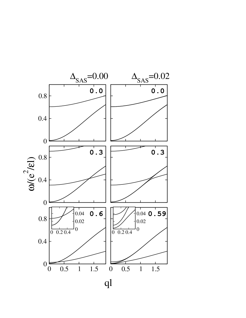
Figure 2: The collective-mode dispersions of the charge-unbalanced $\nu=2$ bilayers in perpendicular field – ferromagnetic phase. The dispersions in the left column are given for a system with $\Delta^{0}_{SAS}=0.0(e^{2}/\varepsilon l)$; in the right column – for a system with $\Delta^{0}_{SAS}=0.02(e^{2}/\varepsilon l)$; the Zeeman energy in all panels is $\Delta_{Z}=0.01(e^{2}/\varepsilon l)$; the bias voltage is given in the upper right corner of each panel in units of $(e^{2}/\varepsilon l)$. Some collective-mode dispersions are degenerate. The low-energy, low-wavevector region is shown in the insets.

V Collective-mode dispersions of charge-unbalanced $\nu=2$ bilayers, $\Delta\neq 0$, $Q_{||}=0$

The Hamiltonian of the charge-unbalanced $\nu=2$ bilayer systems in the presence of interlayer tunneling does not commute with the $I^{z}+S^{z}$ operator. The symmetry considerations that we used to obtain an analytical solution for the density-response function of the $\nu=2$ bilayers in the absence of tunneling cannot be used to simplify Eq. (48) when tunneling is present. We therefore use numerical techniques to calculate the dispersion relations of the charge-unbalanced $\nu=2$ bilayers with finite interlayer tunneling. Much insight into the numerical results can be gained by comparing the collective-mode dispersions in the systems with tunneling to the analytical results for the systems without tunneling. The comparison is presented in Figs. 2, 3, and 4, for the ferromagnetic, many-body, and spin-singlet phases, respectively. The sets of plots in each figure are arranged in two columns: In the left column, we plot the dispersion curves of a system with no tunneling. The dispersions of a system with tunneling are given in the right column. In all the plots, the Zeeman energy is set at $\Delta_{Z}=0.01(e^{2}/\varepsilon l)$; the external bias voltage is given in the upper right corner of each panel.

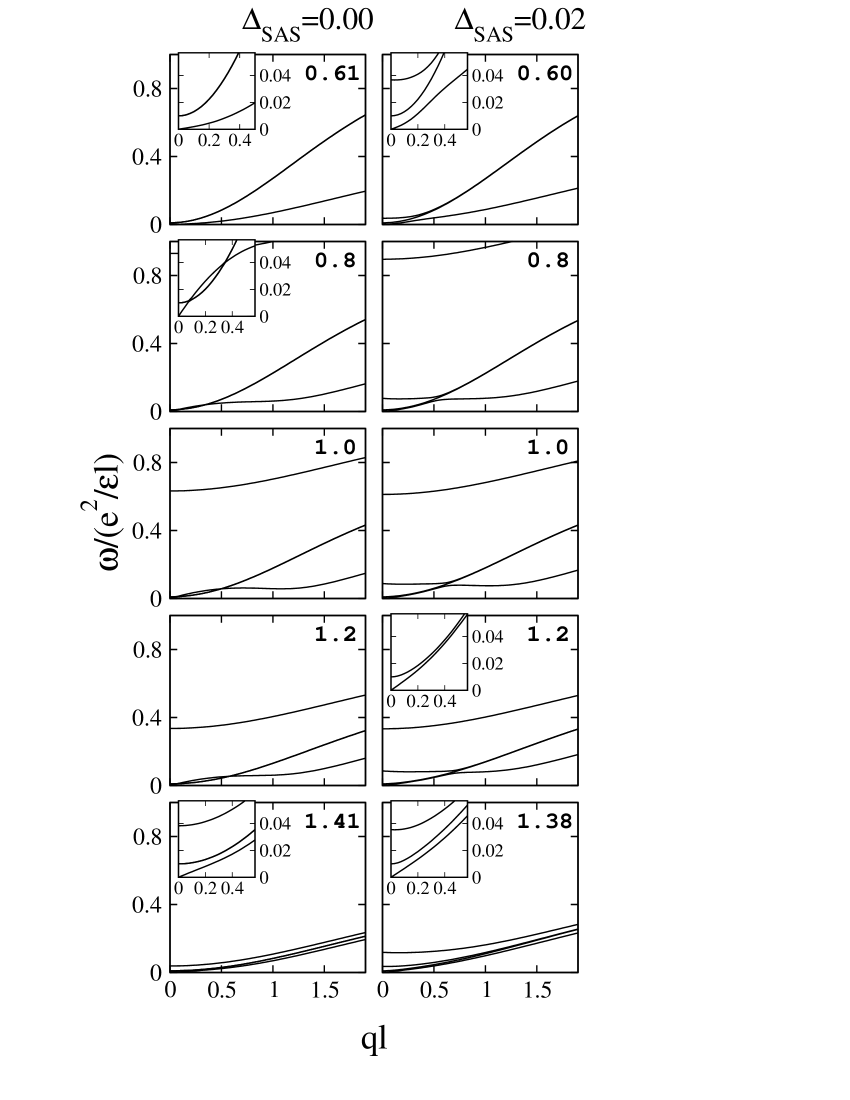
Figure 3: The collective-mode dispersions of the charge-unbalanced $\nu=2$ bilayers in perpendicular field – many-body phase. The dispersions in the left column are given for a system with $\Delta^{0}_{SAS}=0.0(e^{2}/\varepsilon l)$; in the right column – for a system with $\Delta^{0}_{SAS}=0.02(e^{2}/\varepsilon l)$; the Zeeman energy in all panels is $\Delta_{Z}=0.01(e^{2}/\varepsilon l)$; the bias voltage is given in the upper right corner of each panel in units of $(e^{2}/\varepsilon l)$. Some collective-mode dispersions are degenerate. The low-energy, low-wavevector region is shown in the insets.

V.1 Ferromagnetic phase

In Figure 2, we present the dispersion curves obtained in the ferromagnetic phase. While the ferromagnetic ground state does not change as the bias voltage is increased, the collective-mode dispersions demonstrate the evolution of the inter-subband energetics that eventually leads to a phase transition. The top two panels of Fig. 2 show the dispersion curves in the absence of bias voltage. In the absence of tunneling, we can identify the lower curve as the degenerate $1\rightarrow 3$ and $2\rightarrow 4$ excitations, that have a gap equal to the Zeeman energy as $q\rightarrow 0$. The Zeeman gap is hard to discern in the figure, since scale of the Zeeman energy is very small in comparison with the energy scales of the other excitations. The upper curve represents the excitations $1\rightarrow 4$ and $2\rightarrow 3$ that are degenerate in the absence of tunneling and bias voltage. When a small amount of tunneling is present, the degeneracy of the dispersion curves is lifted, and the curves are split by an energy of order ${\cal O}(\Delta_{SAS}^{2}/F_{-})$ — a minute energy difference, not visible on the scale of the figure.

As the bias voltage is increased, as was discussed in the previous section, in the absence if tunneling, the splitting between the dispersions of the $1\rightarrow 4$ and $2\rightarrow 3$ modes increases linearly with the voltage. Thus, at $\Delta_{V}=0.3(e^{2}/\varepsilon l)$, the splitting of the upper branches is very large and apparent. The Zeeman branch, $1\rightarrow 3$ and $2\rightarrow 4$, in the systems without tunneling, remains degenerate for any bias voltage. Note that, in the absence of tunneling, the dispersion curve of the $2\rightarrow 3$ mode crosses the Zeeman branch clearly without interacting with it. The situation changes when tunneling is present: the (approximately) $2\rightarrow 3$ mode develops an anti-crossing with one of the modes of the Zeeman branch. The interactions between different excitations are allowed in the presence of tunneling by the broken symmetry of the Hamiltonian: when the tunneling term is present, the operator $I^{z}+S^{z}$ does not commute with the Hamiltonian; the eigenvalues of the operator are, therefore, no longer good quantum numbers of the excited states. Nevertheless, one mode always stays independent of other excitations: One can see that, in the states with finite magnetization, Figs. 2 and 3, the spin-wave mode, identified by the Larmor minimum at the Zeeman energy, is always decoupled from the other modes. This is a consequence of the up-down, left-right symmetry of the Hamiltonian mentioned in the Sec. IV.5 and preserved in the presence of tunneling. This symmetry maps the excitation $1\rightarrow 3$ to $4\rightarrow 2$. The mapping results in a special form of the density-response matrix that always separates out one Zeeman mode.

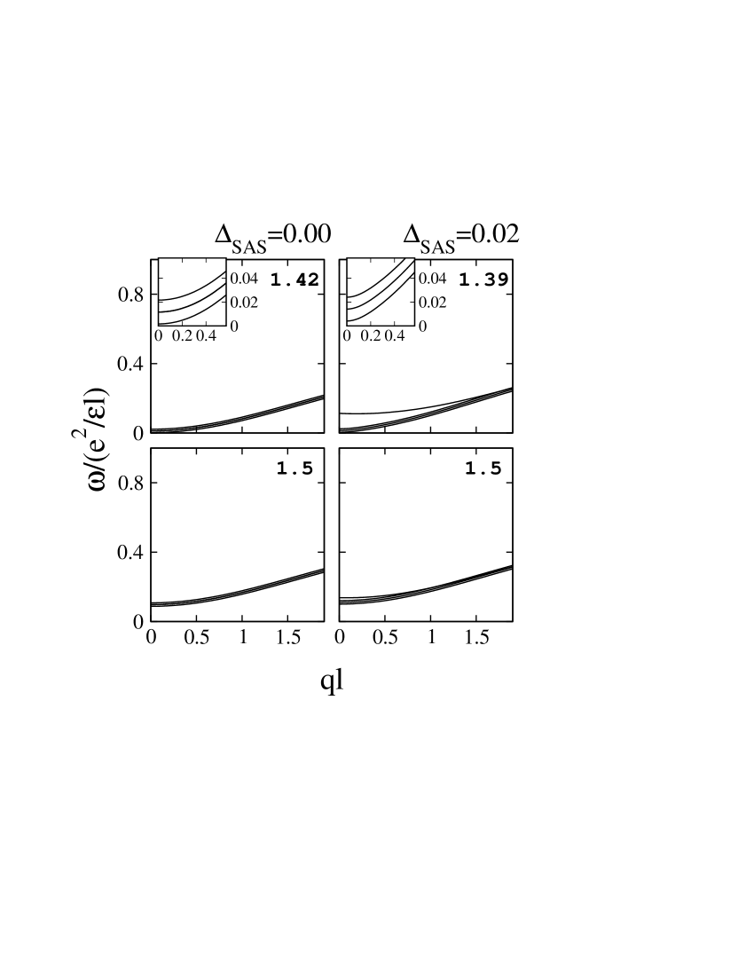
Figure 4: The collective-mode dispersions of the charge-unbalanced $\nu=2$ bilayers in perpendicular field – spin-singlet phase. The dispersions in the left column are given for a system with $\Delta^{0}_{SAS}=0.0(e^{2}/\varepsilon l)$; in the right column – for a system with $\Delta^{0}_{SAS}=0.02(e^{2}/\varepsilon l)$; the Zeeman energy in all panels is $\Delta_{Z}=0.01(e^{2}/\varepsilon l)$; the bias voltage is given in the upper right corner of each panel in units of $(e^{2}/\varepsilon l)$. Some collective-mode dispersions are degenerate. The low-energy, low-wavevector region is shown in the insets.

V.2 Many-body canted and $I$-phases

As the voltage is increased further, the gap of the $2\rightarrow 3$ mode decreases until it disappears. The softening of the mode signals the onset of a many-body phase — the $I$-phase in the system without tunneling and the canted phase in the presence of tunneling. The critical voltage is higher in the system without tunneling, since, when the tunneling is present, it works in concert with the bias voltage to stabilize the spin-singlet phase and destabilize the ferromagnetic phase. The details of the collective mode dispersions as the gap of the $2\rightarrow 3$ mode approaches zero around $\Delta_{V}\approx 0.6(e^{2}/\varepsilon l)$ are given in the insets of the bottom two panels of Fig. 2. In both insets, one can clearly see the Zeeman branch with the gap at the Zeeman energy, $\Delta_{Z}=0.01(e^{2}/\varepsilon l)$. In the absence of tunneling, Zeeman branch is degenerate; when tunneling is finite, the degeneracy is lifted by the interaction with the $2\rightarrow 3$ branch near $q=0$. The interaction of the $2\rightarrow 3$ excitation with the superposition of the $1\rightarrow 3$ and $2\rightarrow 4$ excitations result in an earlier onset of the many-body phase and a mixed mode with a large gap around $q=0$. When the bias voltage is increased a little above $\Delta_{V}\approx 0.6(e^{2}/\varepsilon l)$, the system undergoes a phase transition into the many-body phase. The collective-mode dispersions for the $\nu=2$ bilayers in the many-body phase are given in Fig. 3. Right after the transition the velocity of the Goldstone mode is very low, but it rapidly increases as the system is taken deeper into the many-body phase by an increasing bias voltage. Near the transition, the velocity of the mode increases faster in the canted phase, than in the $I$-phase. In the canted phase, however, because of the inter-mode interactions, the velocity soon reaches nearly a constant, while in the $I$-phase it continues increasing until approximately the middle of the $I$-phase. As the system gets closer to the transition to the spin-singlet phase, the Goldstone-mode velocity goes to 0 in the reverse fashion.

Another effect of the broken-symmetry of the Hamiltonian in the presence of tunneling is the further widening of the gap that develops in the mode that splits off the Zeeman branch as a consequence of the mixing with the other modes. This gap is much larger than $\Delta_{SAS}$ and is therefore due to the interactions. Finite $\Delta_{SAS}$ in this case mainly serves to break the symmetry of the Hamiltonian. This, “third”, mode develops a non-analyticity at $q=0$ and a ring of shallow roton minima, degenerate for all directions of $q$.

The roton minimum that, as we showed in the previous subsection, characterizes the $I$-phase is inherited by the low-tunneling canted phase. It is however less deep in the canted phase, and gradually disappears as tunneling is increased until it becomes more important than the bias voltage (i.e. when the bias voltage does not result in a significant charge imbalance within the many-body phase). Another feature to observe is the lowering of the energy of the highest-energy mode. Its energy scale changes dramatically as one sweeps across the many-body phase by increasing the bias voltage. Around the boundary between the ferromagnetic phase and the many-body phase, the gap of the highest-energy mode is two orders of magnitude larger than $\Delta_{Z}$ (it is rather of ${\cal O}(\Delta_{V})$), but at the boundary of the many-body phases and the spin-singlet phase, the gap decreases to $2\Delta_{Z}$.

V.3 Spin-singlet phase

When the bias voltage is around $\Delta_{V}\approx 1.4(e^{2}/\varepsilon l)$, the system undergoes a phase transition from the many-body to the spin-singlet phase. At this point the Goldstone branch develops a gap. The Goldstone mode becomes the lowest of the three spin-triplet excitations above the spin-singlet ground state. As can be seen in the insets, the three modes are separated by $\Delta_{Z}$. In the absence of tunneling the $S^{z}=0$ spin triplet is degenerate with the only allowed spin-singlet excitation. When tunneling is present, the energy of the spin-singlet excitation is affected by the interactions; it slowly approaches the energy of the $S^{z}=0$ spin triplet as the increasing bias voltage turns the interlayer-phase coherent spin-singlet state at $\Delta_{SAS}\neq 0$ into a $\nu=2$ spin-unpolarized monolayer state.

VI Collective-mode dispersions of charge-unbalanced $\nu=2$ bilayers in tilted field

Figure 5: The collective-mode dispersions of the charge-unbalanced $\nu=2$ bilayers in tilted field – evolution across the $C1$–$C2$ phase transition. The dispersions are given for a system with $\Delta^{0}_{Z}=0.01(e^{2}/\varepsilon l)$, $\Delta^{0}_{SAS}=0.06(e^{2}/\varepsilon l)$, and $\Delta_{V}=0.8(e^{2}/\varepsilon l)$. The strength of the in-plane component of the tilted magnetic field is given by the wavevector $Q_{||}$, which, for every set of dispersion curves, is represented by a number in the units of $1/l$. When $Q_{||}l\leq 0.96$, the system is in the $C1$ phase; when $Q_{||}l>0.96$, it is in the $C2$ phase. In the bottom left panel, the dotted line is for comparison of the dispersion curves in the $C2$ phase to those in the $I$-phase.

As we discussed in Sec. II above and in Ref. Lopatnikova et al., 2003, tilting the magnetic field away from the normal to the plane of the bilayer system leads to new phases and, in charge-unbalanced systems, phase transitions. In the charge-balanced $\nu=2$ bilayers, the tilted fields do not change the topology of the phase diagram. The interlayer phase coherent phases – spin-singlet and canted – become commensurate, and the ferromagnetic state is not affected by the in-plane field. In commensurate interlayer phase coherent phases, the interlayer exchange interactions are effectively destabilized by the in-plane field, and the phase-space volume of the canted phase decreases as the magnetic field is tilted. The weakening of interlayer exchange interactions renormalizes collective mode dispersions of the charge-balanced $\nu=2$ bilayers but does not result in interesting new features.

The presence of a finite in-plane component of the magnetic field produces more interesting effects in charge-unbalanced systems. When tunneling is strong enough, the in-plane field induces a new phase transition between the simple commensurate phase, $C1$, stable at low in-plane fields, and the spin-isospin commensurate phase, $C2$, more favorable at higher in-plane fields. As is shown in Fig.  1 and discussed in depth in Ref. Lopatnikova et al., 2003, the phases $C1$ and $C2$ are connected to each other, and the first-order transition between them terminates at a critical point. To further study this first-order transition, we obtain a series of collective-mode dispersions, calculated for the $C1$ and $C2$ states as the in-plane field is increased. We also obtain the collective-mode dispersions at the critical point terminating the $C1$–$C2$ transition.

VI.1 Collective-mode dispersions across the $C1$–$C2$ phase transition

The evolution of the dispersion curves within the canted phases as the magnetic field is tilted is given in Fig. 5. We choose a system with $\Delta^{0}_{Z}=0.01(e^{2}/\varepsilon l)$ and $\Delta^{0}_{SAS}=0.06(e^{2}/\varepsilon l)$, and hold the external bias voltage at $\Delta_{V}=0.8(e^{2}/\varepsilon l)$, so that the system is approximately in the middle of the canted phase (c.f. Figs. 1). For each probed point on the phase diagram in Fig. 1, we plot in Fig. 5 the cross-sections of the collective-mode dispersions in two directions – perpendicularly to the in-plane field (in the $\hat{x}$ direction in our calculations), and in the direction parallel to it (the $\hat{y}$ direction); these plots are given side by side. The measure of the magnitude of the in-plane component of the magnetic field, the wavevector $Q_{||}$, is given as the number in the left panel.

The top two panels show the collective-mode dispersions in perpendicular magnetic field. In perpendicular field, the dispersions are the same in all directions, so the dispersion curves in the left and the right panels coincide. One can see the features discussed for the canted phase in the charge-unbalanced $\nu=2$ bilayers (Sec. IV): the linearly dispersing Goldstone mode that has a roton minimum around $ql\approx 1$, characteristic of charge-unbalanced systems; the spin-wave mode that decouples from the other three modes and has a gap equal to the Zeeman energy (the resolution of the figure does not allow to see the Zeeman splitting because of the relatively small Zeeman energy); the large interaction-induced gap at $q=0$ of the third mode. The highest-energy mode is not visible in this figure.

When the magnetic field is tilted, the collective modes start changing: they become asymmetric with respect to $q_{\perp}\rightarrow-q_{\perp}$. The velocity of the Goldstone-mode in the negative $q_{\perp}$-direction becomes greater than that in the positive $q_{\perp}$-direction. The roton minima also become asymmetric — they develop a lowest point in the negative $q_{\perp}$-direction. This behavior is reminiscent of the behavior of the collective-mode dispersions of a (charged) superfluid under the influence of an external electromagnetic gauge field, ${\bf A}$. In a superfluid, much like in the $\nu=2$ bilayers in the canted phase, a U(1) symmetry is spontaneously broken. The symmetry breaking results in the formation of a linearly dispersing Goldstone mode. When an external field is applied to a charged superfluid, the superfluid order parameter acquires a twist, $e^{i\frac{e}{c}{\bf A}\cdot{\bf x}}$, and the Goldstone mode acquires an anisotropy:

$$\omega_{\bf k}=|{\bf k}|\sqrt{v_{0}^{2}-\frac{1}{2}(\frac{\hbar e}{mc})^{2}|{\bf A}|^{2}}-\frac{\hbar e}{mc}{\bf A}\cdot{\bf k},$$ (81)

where $v_{0}$ is the initial velocity of the Goldstone mode. While the in-plane field does not couple to the symmetry-breaking order parameters in $\nu=2$ bilayers in the same way it does in a superfluid, it does result in winding phase factors $e^{iQ_{S}X}$, $e^{iQ_{I}X}$, and $e^{i(Q_{S}\pm Q_{I})X}$. Because of the gauge symmetry of our system, an equivalent picture can be drawn up, in which fictitious gauge fields proportional to $Q_{S}$, $Q_{I}$, and $Q_{S}\pm Q_{I}$ couple to the corresponding (uniform) order parameters. In fact, this is exactly what we have done, when we chose to work in the basis of the creation-annihilation operators $f_{\alpha}$ (see Sec. III and Eq. (21)), in terms of which the ground state is uniform.

Because the in-plane field generates different phase factors ($e^{iQ_{S}X}$, $e^{iQ_{I}X}$, and $e^{i(Q_{S}\pm Q_{I})X}$) for different order parameters, the $\nu=2$ bilayer system is somewhat more complicated than a model superfluid. It is clear in Fig. 5, that different collective-mode branches (and different parts of the branches) do not respond to the presence of an in-plane field in the same way. Thus, the Goldstone mode “tilts” to the right in Fig. 5, while the roton minima “tilt” to the left. An effective theory of coupled superfluids that would explain the behavior of the collective modes, as well as the $C1$–$C2$ superfluid-superfluid phase transition is a potential direction of future research.

In addition to the anisotropies, the application of the in-plane field results in an increased Zeeman mode gap, $\Delta_{Z}=\Delta^{0}_{Z}\sqrt{1+Q_{||}^{2}l^{4}/d^{2}}$. It is also apparent, especially at higher in-plane field, that the minimum of the Zeeman mode shifts from $q_{\perp}=0$ to $q_{\perp}=Q_{S}$. This effect is also a consequence of the our choice of the gauge. As was mentioned in Sec. III, the density response function $\chi_{\alpha\beta\gamma\delta}({\bf k};\tau)$ that we calculate is gauge-dependent, because it is the response of the system to the excitation with the density operator $\rho_{\alpha\beta}({\bf k})$. This density operator is related to the physical density operators not only through a linear transformation, but also through a shift of the wavevector (Eq. (23)). A real excitation therefore will pick out signals from different dispersion curve branches (according to allowed symmetries) at different wavevectors. Thus, for example, the physical response function for a real spin-flip excitation of wavevector ${\bf k}$ is a superposition of the $\chi_{\alpha\beta\gamma\delta}({\bf q};\tau)$ at wavevector ${\bf k}+Q_{S}\hat{x}$

$$\chi_{\mu\downarrow\,\mu\uparrow;\mu\downarrow\,\mu\uparrow}({\bf k},\tau)=-g\langle T\rho_{\mu\downarrow\,\mu\uparrow}({\bf k},\tau)\rho^{{\dagger}}_{\mu\downarrow\,\mu\uparrow}({\bf k},0)\rangle=$$

$$=e^{i\mu Q_{||}k_{y}l^{2}}\sum_{\alpha\beta\gamma\delta}(z^{\alpha}_{\mu\downarrow})^{*}z^{\beta}_{\mu\uparrow}(z^{\delta}_{\mu\uparrow})^{*}z^{\gamma}_{\mu\downarrow}\,\chi_{\alpha\beta\gamma\delta}({\bf k}+Q_{S}\hat{x},\tau)).$$

The dispersion curves in the direction parallel to the in-plane field stay symmetric with respect to $q_{||}\rightarrow-q_{||}$. As the tilt-angle is increased, they change mainly because the minimum of the Zeeman and other branches shift away from the $q_{\perp}=0$ plane plotted in the right column of Fig. 5.

As the magnetic field is tilted further, the anisotropy of the Goldstone-mode velocity becomes greater, and the energy of its roton minimum around $q_{\perp}l\approx-1$ decreases. Near the $C1$–$C2$ phase transition, $Q_{||}=0.96$, the roton minimum becomes lower than the Zeeman energy. However, before it reaches zero and the system becomes unstable, the phase transition to the $C2$ phase occurs, marked by an abrupt change in the collective-mode dispersions. The entire picture is effectively shifted by $Q_{S_{C2}}-Q_{S_{C1}}$ (see Fig. 5) in the positive $q_{\perp}$ direction. A Goldstone mode appears in place of the roton minimum, and a roton-minimum replaces the Goldstone mode. The minimum of the Zeeman mode jumps from $Q_{S_{C1}}$ to $Q_{S_{C2}}$, as expected from Eq. (VI.1) and Fig. 5.

Figure 6: The collective-mode dispersions of the charge-unbalanced $\nu=2$ bilayers in tilted field at a critical point terminating the $C1$–$C2$ transition. The dispersions are given for a system with $\Delta^{0}_{Z}=0.01(e^{2}/\varepsilon l)$ and $\Delta^{0}_{SAS}=0.06(e^{2}/\varepsilon l)$. The critical point for this system occurs at $\Delta_{V}=0.5328$ and $Q_{||}=0.9362$; $Q_{S}\approx 0.474$ for these parameters. The top plot zooms in on the long-wavelength region, to demonstrate the $q^{3}_{\perp}$ dependence of the Goldstone-mode dispersions in the positive $q_{\perp}$ direction.

As the in-plane field is increased further, the roton minimum of the Goldstone branch becomes less deep – it approaches the Zeeman energy, $\Delta_{Z}$, from below. When the in-plane component of the magnetic field becomes large, $Q_{||}\approx 2$, the $C2$ phase becomes very close to an $I$-phase. This is reflected in the collective mode dispersions. In the bottom panels of Fig. 5, at $Q_{||}$ we can see the symmetry of the Goldstone branch reappearing (the dotted line in Fig. 5 is given as a guide to the eye). One of the Zeeman branches of the $I$-phase forms an anti-crossing with the Goldstone branch at $q_{\perp}\approx 1$. When $Q_{||}\approx 2$ the Zeeman modes and the Goldstone branch become nearly decoupled. The Zeeman branches in our calculation have a minimum at $Q_{S}\approx Q_{||}$ in high magnetic fields. This is again the gauge effect we described above. Zeeman modes shifted by $-Q_{S}$, as they would be in terms of physical densities, would restore the $I$-phase-like appearance of the collective-mode dispersions deep in the $C2$ phase.

VI.2 Collective-mode dispersions at the critical point

In the last part of this section, we consider the collective mode dispersions at the critical point. Again, we use a bilayer system with $\Delta^{0}_{Z}=0.01(e^{2}/\varepsilon l)$ and $\Delta^{0}_{SAS}=0.06(e^{2}/\varepsilon l)$. The critical point for this sample occurs at $\Delta_{V}=0.5328$ and $Q_{||}=0.9362$; $Q_{S}\approx 0.474$ for these parameters. The spin-wave wavevector $Q_{S}$ is hard to define precisely at the critical point, since the energy profile as a function of $Q_{S}$ is very flat: $~{}(Q_{S}-Q_{S_{c}})^{4}$. The “flatness” of the energy as a function of the spin-wave wavevector $Q_{S}$ implies the existence of very soft spin-wave fluctuations. Indeed, as shown in Fig. 6, the velocity of the Goldstone mode in the positive $q_{\perp}$ direction becomes 0 (and the next-order in $q_{\perp}$ emerges: $\omega\propto q_{\perp}^{3}$).

VII Conclusions

In summary, we have obtained the collective mode dispersions of the charge-unbalanced $\nu=2$ bilayers in tilted magnetic fields using the time-dependent Hartree-Fock approximation (Figs. 2–6). The collective modes possess a number of characteristics that can be observed in light scattering experiments — such as softening modes and roton minima. Thus, the novel phase $C1$–$C2$ phase transition, discussed at length in Ref.Lopatnikova et al., 2003, is signaled by a near-softening of a roton minimum.

The collective-mode dispersions of the $\nu=2$ bilayers in tilted fields exhibit behavior suggestive of a system of coupled superfluids under the influence of an external gauge field. Thus, when the magnetic field is tilted, i.e. a finite in-plane magnetic field is added to the system, the modes become Doppler-shifted (Eq. (81)). The Doppler shift is varies for different modes, reflecting on the fact that the in-plane magnetic field couples to the order parameters of the $\nu=2$ bilayer systems in different ways (see Sec. VI.1).

An interesting future direction of research therefore would be the construction of an effective model with two order parameters that spontaneously break $U(1)$ symmetry. An external gauge field can couple to the order parameters differently, so that when the breakdown of one superfluid occurs, the other superfluid is stable. Such a superfluid transition would be an interesting model for the $C1$–$C2$ transition in the $\nu=2$ bilayers.

References

- (1) Current address, Laurel Ridge Asset Management, New York, NY 10017; alopatnikova@lram.com
- Sarma and Pinczuk (1997) See, for example, A. Pinczuk in Perspectives in Quantum Hall effects S. Das Sarma and A. Pinczuk, eds., (John Wiley & Sons, Inc., New York, NY, USA, 1997).
- (3) See chapters by J. P. Eisenstein, S. M. Girvin, and A. H. MacDonald, in Ref. 1.
- Pellegrini et al. (1997) V. Pellegrini, A. Pinczuk, B. S. Dennis, A. S. Plaut, L. N. Pfeiffer, and K. W. West, Phys. Rev. Lett. 78, 310 (1997).
- Pellegrini et al. (1998) V. Pellegrini, A. Pinczuk, B. S. Dennis, A. S. Plaut, L. N. Pfeiffer, and K. W. West, Science 281, 799 (1998).
- Zheng et al. (1997) L. Zheng, R. Radtke, and S. Das Sarma, Phys. Rev. Lett. 78, 2453 (1997).
- Sarma et al. (1998) S. Das Sarma, S. Sachdev, and L. Zheng, Phys. Rev. B 58, 4672 (1998).
- Burkov and MacDonald (2002) A. A. Burkov and A. H. MacDonald, Phys. Rev. B 66, 115323 (2002).
- Lopatnikova et al. (2003) A. Lopatnikova, S. H. Simon, and E. Demler, preceding paper (2003).
- MacDonald et al. (1999) A. H. MacDonald, R. Rajaraman, and T. Jungwirth, Phys. Rev. B 60, 8817 (1999).
- Kallin and Halperin (1984) C. Kallin and B. I. Halperin, Phys. Rev. B 30, 5655 (1984).
- Côté and MacDonald (1991) R. Côté and A. H. MacDonald, Phys. Rev. B 44, 8759 (1991).
- Côté et al. (1995) R. Côté, L. Brey, H. A. Fertig, and A. H. MacDonald, Phys. Rev. B 51, 13475 (1995).
- Demler et al. (2002) D.-W. Wang, S. Das Sarma, and, E. Demler Phys. Rev. B 66, 195334 (2002).