Configurational Entropy and its Crisis in Metastable States: Ideal Glass Transition in a Dimer Model as a Paragidm of a Molecular Glass

Abstract

We discuss the need for discretization to evaluate the configurational entropy in a general model. We also discuss the prescription using restricted partition function formalism to study the stationary limit of metastable states. We introduce a lattice model of dimers as a paradigm of molecular fluid and study metastability in it to investigate the root cause of glassy behavior. We demonstrate the existence of the entropy crisis in metastable states, from which it follows that the entropy crisis is the root cause underlying the ideal glass transition in systems with particles of all sizes. The orientational interactions in the model control the nature of the liquid-liquid transition observed in recent years in molecular glasses.

1 Introduction

Glass transition (GT) in a glass-forming system such as a single-component liquid (for example, water and silicate melts) remains a controversial long-standing problem, even after many decades of active investigation and presents one of the most challenging problems in theoretical physics[1-4]. In particular, the existence of high and low density forms of viscous water [5] is a consequence of a liquid-liquid transition in the glassy state [6]. As the liquid is cooled below its melting temperature $T_{\text{M}}$ with sufficient care so that the crystallization does not occur, the liquid gets in a metastable liquid (ML) state, commonly known as the supercooled liquid (SCL) state, which is disordered with respect to its ordered crystalline phase (CR). The glass transition occurs in SCL at a temperature T${}_{\mathrm{G}},$ which is usually about two-thirds of the melting temperature $T_{\text{M}}$ for the liquid. The relaxation time and the viscosity increase by several orders of magnitudes, typically within a range of a few decades of the temperature as it is lowered, and eventually surpass experimental limits. In other words, the system basically freezes at T_G without any anomalous changes in its thermodynamic densities like its specific volume or the entropy density. In particular, no spatial correlation length has been identified so far that would diverge near the transition at T_G. On the other hand, mode-coupling theory [7] shows a dynamic slowdown at a temperature T_MC much higher than T_G but lower than $T_{\text{M}}$, and a loss of ergodicity. The relationship between T_MC and T_G is not understood at present, although attempts have been made recently [8-10] to understand it partially in connection with long polymers. The free volume falls rapidly near T_MC for long polymer fluids, with the nature of the drop becoming singular in the limit of infinitely long polymers. The glass transition occurs at a temperature $T_{\text{K}}<$T_MC where the configurational entropy vanishes, even if the polymer liquid is incompressible [8] at all temperatures. The configurational entropy $S(T),$ by definition [3], is the entropy that is used to define the configurational partition function (PF)

$$Z(T)\equiv\frac{1}{V^{N}}\int^{{}^{\prime}}e^{-\beta E}d^{N}\{\mathbf{r\},}$$ (1)

in the canonical ensemble for a system of $N$ particles in a volume $V$ at a given temperature $T$. The prime indicates that the integration is over distinct configurations, $E(\{\mathbf{r}_{i}\})$ represents the potential energy in a given configuration $\{\mathbf{r}_{i}\}$ determined by the instantaneous positions of all the particles, $d^{N}\{\mathbf{r\}}$ represent integrations with respect to $N$ positions $\mathbf{r}_{i}$ of the particles, and $\beta\equiv 1/T$, $T$ being the inverse temperature in the units of the Boltzmann constant $k_{\text{B}}.$ The number of distinct configurations $W(E)dE$ with energy in the range $E$ and $E+dE$ determines the configurational entropy $S(E)\equiv\ln W(E)dE\simeq\ln W(E)$ [11] in the corresponding microcanonical ensemble at a given configurational energy $E.$ For the state to be realizable in Nature, it is obvious that the number of states must be a positive integer. Hence, we must always have $S(E)\geq 0.$ The average energy $\overline{E}(T)$ in the canonical ensemble gives the configurational entropy $S(T)\equiv S[\overline{E}(T)]$ in that ensemble, and must also be non-negative.

The loss of configurational entropy seems to be a generic phenomenon. The thermal data for various systems capable to form glassy states exhibit an entropy crisis discovered by Kauzmann[1], in which a rapid entropy drop to a negative value occurs below the glass transition temperature in SCL [2,4]. This strongly suggesting a deep connection between thermodynamics and GT, since thermodynamics requires the entropy to decrease as the temperature is lowered. Consequently, it is tempting to treat the experimentally observed GT as a manifestation of an underlying thermodynamic ideal glass transition, which is invoked to avoid the genuine entropy crisis when the SCL configurational entropy $S_{\text{SCL}}<0$ below a non-zero temperature $T=T_{\text{K}}.$ Negative $S_{\text{SCL}}$ implies that such states are unrealizable in Nature [8-10,12-13], which is what the entropy crisis signifies. Free volume, which also seems to decrease with lowering the temperature [1-2,4], does not seem to be the primary cause, though it may be secondary, behind GT as shown recently [10], as there is no thermodynamic requirement for it to decrease with the lowering of the temperature.

The entropy crisis and the resulting ideal GT have only been substantiated so far in two exact calculations. The first one is an exact calculation by Derrida on an abstract model known as the random energy model [14]. The second one is an explicit exact calculation by Gujrati and coworkers [8-10] in long semiflexible polymers, which not only satisfies the rigorous Gujrati-Goldstein free energy upper bound [15] for the equilibrium state, but also yields $S_{\text{SCL}}(T)<0$ below a positive temperature $T=T_{\text{K}}$ [13]. An earlier demonstration of the crisis in polymers by Gibbs and DiMarzio [16] was severely criticized by Gujrati and Goldstein [15] for its poor approximation that violates the rigorous Gujrati-Goldstein bounds, thus raising doubts about their primary conclusion of demonstrating an entropy crisis [13]. Despite its limitation, the work has played a pivotal role in elevating the Kauzmann entropy crisis from a mere curious observation to probably the most important mechanism behind the glass transition, even though the demonstration was only for long molecules. Unfortunately, the criticism by Gujrati and Goldstein has been incorrectly interpreted by some workers [17] by taking their bounds to be also applicable to metastable states in polymers. To overcome the bounds, DiMarzio and Yang have suggested to replace the unrealizability condition $S_{\text{SCL}}<0$ by an arbitrary condition $S_{\text{SCL}}<S_{\text{c0}}$ for the entropy crisis, where $S_{\text{c0}}$ is some small critical value [13]. This is not the correct interpretation of the Gujrati-Goldstein bounds. These bounds are only for the equilibrium states, since they are obtained by considering Gujrati-Goldstein excitations in CR; they are not applicable to SCL, which represents a disordered state.

A glass can be thought as a disordered or amorphous solid [18]. There are no general arguments [18-19] to show that thermodynamically stable states must always be ordered, i.e., periodic. The remarkable aperiodic Penrose tilings of the plane, for example, by two differently but suitably shaped tiles are stable. Nevertheless, it appears that most amorphous states in systems that crystallize have much higher internal energy or the enthalpy than the corresponding crystal, even near or at absolute zero [1,18]. Thus, we will consider amorphous solids, i.e. glasses, as representing metastable, rather than stable states in this work. The higher energy of the glass has been used as the basis of a recent thermodynamic proof [12] that there must exist a non-zero Kauzmann temperature $T_{\text{K}}$ below which the configurational entropy of the disordered or the amorphous state of the system becomes negative.

It should be stressed that the glass transition is ubiquitous and is also seen in small molecules. Therefore, it is widely believed that the entropy crisis also occurs in molecular liquids. However, no such entropy crisis has ever been demonstrated in any explicit calculation for small molecules [4]. This is highly disconcerting and casts doubts on the importance of the entropy crisis for GT in systems consisting of particles of any size. It is this lack of explicit demonstration of the entropy crisis in molecular liquids that has motivated this work.

There is a clear need to settle whether the entropy crisis is generic or not for molecules of all sizes. An explicit calculation without any uncontrollable approximation such as an exact calculation for small molecules will go a long way to settle the matter once for all. Without such a calculation, our understanding of GT cannot become complete. An exact calculation demonstrating a positive Kauzmann temperature for small molecular fluids would be a major accomplishment. The other motivation for the work is to carefully define the configurational entropy so that is satisfies $S(T)\geq 0$ for states that are realizable in Nature. Its violation is then argued as a trigger for the glass transition.

Our aim here is to fill this gap in our understanding by demonstrating the existence of an entropy crisis in an explicit exact calculation on a system of classical dimers as a paradigm of a molecular liquid. In conjunction with our earlier demonstration of the entropy crisis in infinitely and also very long polymer system, our calculation, thus, finally enshrines the Kauzmann entropy crisis ( negative $S_{\text{SCL}}$ implying that such states are unrealizable in Nature) as the general underlying thermodynamic driving force for GT in molecules of all sizes. It should be stated that recent computer simulations have not been able to settle the issue clearly [20]. Our investigation also enables us to draw important conclusions about the role orientational order plays in liquid-liquid (L-L) phase transitions that have been observed recently in many atomic and molecular liquids [21-22]. It has gradually become apparent that the short-ranged orientational order in supercooled liquids plays an important role not only in the formation of glasses but also in giving rise to a liquid-liquid phase transition. Tanaka [23] has proposed a general view in terms of cooperative medium-ranged bond ordering to describe liquid-liquid transitions, based on the original work of Nelson [24]. Thus, we will also consider orientational order in this work.

It is fair to say that there yet exists no completely satisfying theory of the glass transition [3-4,25] even though some major progress has been made recently [26-30,8-10,12]. Theoretical investigations mainly utilize two different approaches, which are based either on thermodynamic or on kinetic ideas. The two approaches provide an interesting duality in the liquid-glass transition, neither of which seems complete. We discuss below briefly some of the most promising theories based on these approaches.

1.1 Free Volume Theory

The most successful theory that attempts to describe both aspects with some respectable success is based on the ”free-volume” model of Cohen and Turnbull [31]. The concept of free volume has been an intriguing one that pervades throughout physics but its consequences and relevance are not well understood [32], at least in our opinion, especially because there is no consensus on what various workers mean by free volume. Nevertheless, GT in this theory occurs when the free volume becomes sufficiently small to impede the mobility of the molecules [33]. The time-dependence of the free-volume redistribution, determined by the energy barriers encountered during redistribution, provides a kinetic view of the transition, and must be properly accounted for. This approach is yet to be completed to satisfaction. Nevertheless, assuming that the change in free volume is proportional to the difference in the temperature $T-T_{V}$ near the temperature $T_{V},$ even though there is no thermodynamic requirement for the free volume to drop as $T$ is lowered [10], the viscosity $\eta(T)$ diverges near $T_{V}$ according to the Vogel- Tammann-Fulcher equation

$$\ln\eta(T)=A_{\text{VTF}}+B_{\text{VTF}}/(T-T_{V}),$$ (2)

where $A_{\text{VTF}}$ and $B_{\text{VTF}}$ are system-dependent constants. This situation should be contrasted with the fact that there are theoretical models [14,8-9] without any free volume in which the ideal glass transition occurs due to the entropy crisis at a positive temperature. Hence, it appears likely that the free volume itself is not the determining cause for the glass transition in supercooled liquids. However, too much free volume can destroy the transition [10]. We will, thus, explore the influence of free volume on the glass transition in this work.

1.2 Thermodynamic Theory

The thermodynamic ideas alone describe GT in terms of the entropy crisis at a positive temperature [1]. The entropy crisis corresponds to a rapid entropy drop to a negative value below the glass transition temperature in the supercooled liquid (SCL) [1-4]. An ideal glass transition at $T_{\text{K}}$ is invoked to avoid the entropy crisis. The entropic view plays a central role in the Adams-Gibbs theory [34], according to which the viscosity $\eta(T)$ above the glass transition depends on a quantity also called the configurational entropy $S_{\text{conf}}(T)$ as follows:

$$\ln\eta(T)=A_{\text{AG}}+B_{\text{AG}}/TS_{\text{conf}}(T),$$ (3)

where $A_{\text{AG}}$ and $B_{\text{AG}}$ are system-dependent constants. The existence of the entropy crisis has been justified in many exact model calculations [14,8-10,16]. An alternative thermodynamic theory for the impending entropy crisis based on spin-glass ideas has also been developed in which proximity to an underlying first-order transition is used to explain the glass transition [26].

In a thermodynamic theory, the glass-forming system is treated as homogeneous, mainly because there appears to be no evidence of any structural changes emerging near GT. From this point of view, a thermodynamic theory gives rise to a homogeneous free energy. However, the fluctuations in it can be used to construct the equations for time-dependence in the system. Thus, the thermodynamic approach can be used to describe the dual aspect of the glass transition. In particular, it should enable us to provide a bridge between the two expressions in (2,3) for the viscosity that are the most widely-used and successful formalism of viscosity in glass-forming liquids.

1.3 Mode-Coupling Theory

The mode-coupling theory [7] is an example of theories based on kinetic ideas in which glass formation is described as a slowing down of liquid’s mobility and its freezing into a unique amorphous configuration at a positive temperature. In this theory, the ergodicity is lost completely, and structural arrest occurs at a temperature T_MC, which lies well above the customary glass transition temperature T_G. Consequently, the correlation time and the viscosity diverge due to the caging effect. The diverging viscosity can be related to the vanishing free volume [31,33], which might suggest that the MC transition is the same as the glass transition. This does not seem to be the consensus at present. Thus, it is not clear if the free volume is crucial for the MC transition. Some progress has been made in this direction recently [10], where it has been shown for long polymers that the free volume vanishes at a temperature much higher than the ideal glass transition. The mode-coupling theory is also not well-understood, especially below the glass transition. More recently, it has been argued that this and mean-field theories based on an underlying first-order transition may be incapable of explaining dynamic heterogeneities.

1.4 Theory vs Experiment/Simulation

In this work, we are interested in the thermodynamic approach to investigate the entropy crisis, according to which the configurational entropy $S_{\text{SCL}}(T)$ vanishes at some positive temperature. It should be remarked that the entropy crisis can only be seen in theoretical calculations, but never in an experiment or simulation, since the latter two always deal with states that are observed or produced, so that the corresponding entropy would never be negative. It is only by extrapolation that the latter two may predict an entropy crisis. The reliability of such extrapolation is debatable, and has been used to argue against an entropy crisis [35-36]. By analyzing experimental data, they have argued on procedural grounds that an entropy crisis in any experiment must be absent, which we agree with. However, such arguments based solely on experimental data or simulation without extrapolation can never shed light on the issue of the entropy crisis, which is purely hypothetical. To verify the existence or non-existence of the crisis, one must resort to theoretical arguments. Several workers [37-38] have argued theoretically that it is not possible to have any entropy crisis, not withstanding the explicit demonstration of it in long polymers, and in the abstract random energy model. The argument due to Stillinger [37], in particular, is forceful though not rigorous [4]. While he concedes that long polymers may very well have an entropy crisis at a positive temperature, he argues for its absence in viscous liquids of small molecules. From a purely mathematical point of view, it is hard to understand how this scenario could be possible. Using the physical argument of continuity, we expect $T_{\text{K}}$ to be a smooth function of the molecular weight. Thus, it does not seem possible that such a function remains zero over a wide but finite range of the size of the molecules, and abruptly becomes non-zero for very large sizes. A function like this must be a singular function. However, no argument that we can imagine can support a particular large molecular size to play the role of the location of such a singularity.

Assuming the entropy in (3) to be the configurational entropy, which is known to vanish in theoretical calculations, then its rapid decrease to zero should give rise to a diverging viscosity, thus providing a connection between the thermodynamic view and  the kinetic view. However, no experimental evidence in support of such a diverging viscosity is known mainly because the relaxation times become much longer than the experimental time limitations. Thus, it does not seem surprising that theoretical predictions of entropy crisis is never going to be seen directly in experiments.

Despite this, the suggestion that the rapid rise in the viscosity is due to a sudden drop in $S_{\text{T}}(T)$ seems very enticing, since both phenomena are ubiquitous in glassy states. The experimental data indicate that $T_{V}$ and $T_{K}$ are, in fact, very close [39], clearly pointing to a close relationship between the rapid rise in the viscosity and the entropy crisis. This deep connection, if true, provides a very clean reflection of the dual aspects of the glassy behavior mentioned above. It also implies strongly that it is the entropy crisis, which is the root cause of the glass transition. This idea got a strong support recently when it was shown that the free volume could not be the root cause for GT in SCL, as the transition can exist even in the absence of the free volume [10]. Thus, we are driven to the conclusion that it should be possible to treat the SCL glass transition within a thermodynamics formalism by demonstrating the existence of the entropy crisis. In other words, if the scenario is valid, we can treat the experimentally observed GT as a manifestation of the underlying ideal glass transition induced by the entropy crisis. The ideal glass transition is a hypothetical transition obtained in the limit of infinite slow cooling, provided the crystal (CR) is forbidden to nucleate. This transition will never be observed in experiments since such cooling rates are impossible to maintain in reality or in simulations since any state generated in simulation will ensure that the entropy is not negative. Thus, experimentally or in simulations, one would never observe the ideal glass transition directly. It can only be inferred either by some sort of extrapolation or by diverging relaxation times in these methods. On the other hand, a theoretical demonstration of an ideal glass transition is possible since neither the time restriction is an issue nor the realizability of a state. The theoretical existence of an ideal glass transition forces us to conclude that the observed glass transitions in experiments are a manifestation of this transition, or in other words, of the entropy crisis. As such, a study of the glass transition within a thermodynamics formalism will enable us to understand glassy phenomena in a systematic and fundamental way.

It should be noted that what one measures in experiments is the difference in the entropy, and not the absolute entropy. Assuming that the entropy is zero at absolute zero in accordance with the Nernst-Planck postulate, one can then determine the absolute entropy experimentally. However, it is well known that SCL is a metastable state, and there is no reason for its entropy to vanish at absolute zero [18]. Indeed, it has been demonstrated some time ago that the residual entropy at absolute zero obtained by extrapolation is a non-zero fraction of the entropy of melting [40], which is not known a priori. Therefore, it is impossible to argue from experimental data that the entropy indeed falls to zero, since such a demonstration will certainly require calculating absolute entropy though efforts continue to this date [35-36].

The layout of the paper is the following. In the next section, we discuss classical statistical mechanical approach to study glass transition and show the need for discretizing both the real and the momentum spaces. We also compare the configurational entropy in (1) and the criterion for the entropy crisis with other definitions and criteria available in the literature. In Section 3, we describe the classical dimer model, and its Husimi cactus approximation is discussed in Section 4. We solve the model exactly on the cactus by using the recursion relation (RR) technique and the results are presented in Section 5. The final section contains discussion of our results and conclusions. The RR’s are deferred to the Appendix.

2 Configurational Partition Function and Entropy Crisis

2.1 Negative Entropy in Continuum Classical Statistical Mechanics

We consider a system of $N$ identical particles $i=1,2,...,N$ confined in a container of volume $V$. The position $\mathbf{r}_{i}$ and momentum $\mathbf{p}_{i}$ of the particle $i$ are treated as continuous variables in classical mechanics. The Hamiltonian of the system is given by

$$H\equiv\underset{i}{\sum}\mathbf{p}_{i}^{2}/2m+E(\{\mathbf{r}_{i}\}).$$ (4)

The first term in (4) represents the kinetic energy $K$. In classical statistical mechanics (CSM), the total partition function (PF) $Z_{\text{T}}$ for the system can be reduced to a product of two different dimensionless integrals as

$$Z_{\text{T}}\equiv Z_{\text{KE}}Z\mathbf{,}$$ (5)

where

$$Z_{\text{KE}}\equiv\frac{V^{N}}{(2\pi\hslash)^{3N}}\int e^{-\beta K}d^{N}\{\mathbf{p\}}$$ (6)

denotes the PF due to the translational degrees of freedom in which $d^{N}\{\mathbf{p\}}$ represents integrations with respect to $N$ momenta $\mathbf{p}_{i}$ of the particles. The prefactor in terms of $\hslash$ is used not only to make $Z_{N}$ dimensionless, but also to explicitly show the correspondence of $Z_{N}$ with the corresponding PF in the quantum statistical mechanics (QSM) in the classical limit $\hslash\rightarrow 0$. Despite the classical limit requirement $\hslash\rightarrow 0$, we are not allowed to set $\hslash=0$ in the final result, but keep its actual non-zero value. Accordingly, some problems remain such as Wigner’s distribution function not being a classical probability distribution, which we do not discuss any further but refer the reader to the literature [41]. Keeping $\hslash$ at its non-zero value avoids infinities as we will see below but in no way implies that we are dealing with quantum effects. In particular, it does not imply that the entropy is non-negative, as can be seen in the following. The PF $Z_{\text{KE}}$ can be written in terms of $W_{\text{KE}}(P)dP$ $\equiv C_{3N}V^{N}P^{3N-1}dP/h^{3N},$ which is usually thought of as representing the number of microstates corresponding to the magnitude of the total momentum $P$ in the range $P$, and $P+dP$ in the 3$N$-dimensional momentum space, as follows:

$$Z_{\text{KE}}\equiv\int W_{\text{KE}}(P)e^{-\beta K}dP;$$ (7)

here $C_{d}\equiv$ $d\pi^{d/2}/\Gamma(d/2+1)$ is a constant due to angular integration in a $3N$-dimensional space. Being a number of states, $W_{\text{KE}}(P)dP$ should be a positive integer, which as we see below is not true. The entropy function is given by $S_{\text{KE}}(P)=\ln W_{\text{KE}}(P)$ [11], where we have used $K\equiv P^{2}/2m.$ In the thermodynamic limit $N\rightarrow\infty$, the integrand in (7) must be maximum. Hence, we look for the maximum of $P^{3N-1}e^{-\beta K}$ by the prescription, known commonly as the saddle point approximation, of equating its derivative to zero. This immediately gives the ideal gas equation for the average kinetic energy $\overline{K}(T)$

$$\overline{K}(T)=(3/2)NT,$$ (8)

which should come as no surprise. For the ideal gas, the total entropy function $S_{\text{T}}(T)$ is given by

$$S_{\text{T-ideal}}(T)=(3N/2)[\ln T+2V/3N+\ln(2\pi me/\sqrt{h})],$$ (9)

while

$$S_{\text{KE}}(T)=(3N/2)[1+\ln T+\ln(2\pi m/h^{2})].$$ (10)

It should be noted that $S_{\text{KE}}(T)$ has the same value at a given temperature for any classical system, regardless of the configurational energy. Thus, in general, the configurational entropy can be always obtained by subtracting $S_{\text{KE}}(T)$ from $S_{\text{T}}(T)$ [10]:

$$S(T)\equiv S_{\text{T}}(T)-S_{\text{KE}}(T).$$ (11)

For an ideal gas, the configurational PF is $Z=V^{N}/N!,$ and the corresponding configurational entropy, which does not depend on $T$ now, is

$$S_{\text{ideal}}=N\ln(Ve/N).$$ (12)

Both entropies are extensive, and so is the total ideal gas entropy $S_{\text{T-ideal}}(T)$. If we set $h=0,$ we encounter an infinity in the entropy at all temperatures in (10). To avoid this, we keep $h$ at its non-zero value. At absolute zero, or for $V/N<1/e$, $S_{\text{T}}\rightarrow-\infty,$ a well-known result of classical statistical mechanics. For $S_{\text{ideal}}$, it appears at first glance that the problem is due to the point-like nature of the particles, which allows us to pack as many particles as we wish in a given fixed volume $V$. This is not true. The problem is due to the continuum nature of the real space. This is easily seen from the exact solution of the 1-d Tonks gas, which is a simple model of non-interacting hard rods, each of length $a$. In one dimension, the configurational entropy $S$ corresponding to $N$ rods in a line segment of length $L$  is given by [42]

$$S_{\text{Tonks}}=N\ln[(L-Na)e/N]$$ (13)

in the thermodynamic limit. Comparison with (12) shows that the only difference is that the total volume $V$ in (12) is replaced by the free volume analog $L-Na$ in 1-dimensional Tonks gas (13). It is clear that the entropy becomes negative as soon as $L/N<1/e+a$ and eventually diverges to $-\infty$ in the fully packed state. Similarly, the problem with $S_{\text{KE}}(T)\rightarrow-\infty$ as $T\rightarrow 0$ is due to the continuum nature of the momentum space.

This problem disappears as soon as we invoke quantum statistical mechanics to describe the total PF, which no longer can be written as product of two or more PF’s as in (5). Here, we consider the number of states $W_{\text{T}}(E_{\text{T}})\geq 1$ as function of the (total) energy eigenvalue $E_{\text{T}}.$ The energy eigenvalue $E_{\text{T}}$ can certainly be broken into the kinetic energy part $K$ and the potential energy part $E$, but such a partition is not possible for the total entropy $S_{\text{T}}(E_{\text{T}})\equiv\ln W_{\text{T}}(E_{\text{T}}).$ Therefore, in general, the notion of the configurational entropy does not make sense in this case. Since we are only concerned with classical statistical mechanics in this work, we will not discuss this point further here.

2.2 Non-negative Entropy in Classical Statistical Mechanics

As shown above, the entropy of a continuum model is invariably negative in classical statistical mechanics, especially at low temperatures; but this has nothing to do with the entropy crisis noted by Kauzmann. Quantum statistical mechanical calculations are not feasible at present to make entropy non-negative. Thus, at present, no theoretical calculation using continuum classical statistical will be able to justify the entropy crisis, as the negative entropy may just be a manifestation of the continuum picture. However, a lattice picture ensures a non-negative entropy for any state that can be realized in Nature. Thus, a lattice model is capable of settling whether an entropy crisis occurs in the metastable state or not.

To define the number of microstates so that it is always greater than or equal to 1, one must discretize the real and momentum spaces carefully. For this purpose, we introduce a short distance $a$ in real space, and a related quantity $b\equiv\hslash/2\pi a$ having the dimension of the momentum so that $ab=2\pi\hslash$; $a$ may be taken as hard sphere of the molecule. We now divide the two spaces into cells of size $a^{3N}$ and $b^{3N},$ respectively. In the discretized space, the number of microstates is nothing but the number of distinct ways the cells are occupied by the particles’ positions and momenta. This number cannot be less than unity if the microstate is realizable in Nature. Hence, the entropy can never be negative if the state occurs in Nature. For example, $C_{3N}P^{3N-1}dP$ is now replaced by the number of cells of size $b^{3N}$ that cover a shell of integer radius $\overline{P}=P/b$, and thickness $b$ (corresponding to the integer thickness $\overline{dP}=dP/b=1)$. This number is $C_{3N}\overline{P}^{3N-1}.$ The equilibrium is obtained by maximizing the integrand

$$I(\overline{P})\equiv\overline{P}^{3N-1}e^{-(\beta b^{2}/2m)\overline{P}^{2}}.$$

Maximizing $I$ is equivalent to maximizing

$$\widetilde{I}\equiv I(\overline{P})/I(1)\equiv\overline{P}^{3N-1}e^{-(\beta b^{2}/2m)(\overline{P}^{2}-1)},$$ (14)

in which $\overline{P}^{2}-1\geq 0.$ It is evident that the maximum of $\widetilde{I}$ at $\beta\rightarrow\infty$ corresponds to $\overline{P}=1,$ and gives $\widetilde{I}$ =1. This is true for all $N$, and will remain true even as $N\rightarrow\infty$. In this limit, higher values of $\overline{P}$ also condense to the state corresponding to the lowest energy density per particle. Thus, the number of microstates at absolute zero is strictly a positive integer. Correspondingly, the entropy is not negative anymore. It is also clear that for small values of $\overline{P}$ (and finite $N$), we cannot differentiate $\widetilde{I}$ with respect to $\overline{P}$ to find the maximum, as $\overline{P}$ cannot be approximated as a continuous variable in this range. Thus, care must be exercised near absolute zero.

A similar conclusion is drawn for the configurational entropy determining $Z$ in (5). It is also easy to see that the total entropy is independent of the choice $a$ or $b$, though its two components are not. As we will see below, we are mostly interested in the configurational entropy, which from the above is seen to depend on $a$. This is an unwanted behavior, since it makes $S(T)$ depend on the somewhat arbitrary parameter $a$. This unwanted property is easily taken care of by normalizing the configurational entropy not by the number of particles, but by the dimensionless volume $\overline{V}\equiv V/a^{3}.$ It is easy to see that $\overline{S}(T)\equiv S(T)/\overline{V}$ is independent of the arbitrary parameter $a$. In the following, we will always interpret the discretized configurational entropy in this normalized sense.

It is now obvious that the entropy must be non-negative for equilibrium states, since these states occur in Nature. This property need not hold for metastable states, for which a negative entropy now will only indicate that the corresponding state is not realizable in Nature; it is no longer a mere consequence of the continuum picture as above. An exact calculation, like the one we carry out in this work, will evaluate the partition function exactly without using the saddle-point method. It will be seen that the entropy is non-negative for the equilibrium state. We will also see that it can become negative for the metastable state, where it will only imply that such a state is not to be observed in Nature. The part of the metastable state with non-negative entropy represents the metastable state that can occur in Nature. Therefore, we will assume in the following that a discretization of the two spaces has been carried out. In particular, a lattice model in which the particle positions are restricted to be on the lattice sites is very useful from this point of view. There is no kinetic energy in the lattice model. Therefore, $S_{\text{KE}}(T)\equiv 0.$ This leaves us with only the configurational entropy, which represents the entire entropy in the lattice model.

2.3 Other Common Definitions of the Configurational Entropy

It should be clear from the above that the configurational entropy is a concept that can only be introduced in classical statistical mechanics. Unfortunately, there is no direct measurement of the configurational entropy of a system. Thus, its experimental determination is a challenge. There is a further complication in that there is a certain amount of confusion and/or ambiguity about its definition. Our definition in (11) is the most natural definition of the configurational entropy for which the requirement $S(T)\geq 0$ can be justified on the ground that the state must be realizable in Nature. We will call this the thermodynamic principle of reality [8-10,12-13]. The configurational entropy represents that part of the total entropy $S_{\text{T}}(T)$, which is due to the configurational degrees of freedom only [3]. The remainder of the entropy $S_{\text{KE}}(T)$ is due to the translational degrees of freedom and must be subtracted from the total entropy to obtain $S(T)$. Thus, there is no ambiguity in its definition.

The ambiguity arises when we need to estimate $S(T)$ by subtracting the contribution $S_{\text{KE}}(T)$ for the following reason. In a solid state like the glass or CR, where the average particle positions are almost fixed, $S_{\text{KE}}(T)$ is a significant part of the total entropy. The latter is customarily known as the vibrational entropy in this context; we assume that the container is stationary. The difference represents the configurational entropy given by (11). If no discretization has been carried out, then $S_{\text{KE}}(T)$ is given by (10) . This will surely create a problem at low temperatures where $S_{\text{KE}}(T)$ and $S(T)$ become negative. Thus, discretization is necessary, and one needs to carry it out before $S_{\text{KE}}(T)$ can be calculated. In that case, we need to normaize the discretized  configurational entropy $S(T)$ by the dimensionless volume $\overline{V}$ as discussed above.

Traditionally, one treats the translational degrees of freedom approximately in a different fashion, at least for CR. The discretization is enforced by treating the resulting motion as giving rise to quantum vibrations about the minimum of the CR configurational energy. [If we treat these vibrations classically, it can be shown immediately that the kinetic energy contribution to the entropy is precisely given by $S_{\text{KE}}(T).]$ Hence, $S_{\text{KE}}(T)$ differs from the vibrational entropy by an amount exactly equal to the configurational entropy, which need not be small. One further assumes that the vibrational modes of SCL are similar to those in CR. One now traditionally defines the SCL configurational entropy by [3]

$$S_{\text{con-}\mathrm{SCL}}(T)\simeq S_{\mathrm{ex,SCL}}(T)\equiv S_{\text{T-}\mathrm{SCL}}(T)-S_{\text{T-}\mathrm{CR}}(T).$$

Some workers identify the SCL configurational entropy by

$$S_{\text{con-}\mathrm{SCL}}^{\prime}(T)\simeq S_{\text{T-}\mathrm{SCL}}(T)-S_{\text{T-}\mathrm{GL}}(T),$$

the excess SCL entropy over the extrapolated entropy of the corresponding glass [43]. Workers using the potential landscape picture define the configurational entropy to be the entropy $S_{\text{IS}}(E_{\text{IS}})$ of inherent structures of a given potential energy $E_{\text{IS}}$ [37]. To obtain this entropy as a function of $T$, a connection between $E_{\text{IS}}$ and $T$ is required.

In this work, we will continue to use $S(T)$ to define the configurational entropy. In a lattice model, which we consider in this work, we bypass the complication due to $S_{\text{KE}}(T)$ all together since there is no kinetic energy on a lattice. Hence, the entire entropy in the lattice model is purely configurational. The role of the dimensionless volume $\overline{V}$ is played by the number of lattice sites $N_{\text{L}}.$

2.4 Metastability Continuation

A partitioning of the total PF into two or more PF’s in CSM, such as in (5), of decoupled degrees of freedom has an important consequence, which we discuss below. We focus on (5), but the discussion is valid for any general partitioning. The total entropy is a sum of the entropies from the two PF’s. The partitioning implies not only that the total entropy at a given temperature is a sum of the entropy contribution due to $Z_{\text{KE}}$ and that due to $Z$, but also that the two contributions are independent. In particular, $S_{\text{KE}}(T)$ remains the same, whether we consider the crystal or the supercooled phase, both of which can exist at the same temperature below $T_{\text{M}}$. This is because CR and SCL are described by $Z,$ and its appropriate modification to be described below, respectively. Hence, we come to a very important conclusion:

In classical statistical mechanics, which is what is conventionally used to analyze metastability, the contribution $S_{\text{KE}}(T)$ to the total entropy $S_{\text{T}}(T)$ from the translational degrees of freedom is the same for various possible phases like SCL or CR that can exist at a given temperature, and is a function only of the temperature $T$.

Thus, from now on, we will only consider the configurational degrees of freedom. Since the heat capacity is non-negative, $S(T),$ and $E(T)$ are monotonic increasing function of $T$, and must reach their minimum values at absolute zero. Hence, CR must be in the state with energy $E_{0},$ for which we take $S_{\text{CR}}(T=0)=0.$ This requires taking $W(E_{0})=1.$ Thus, $E_{0}$ sets the zero of the temperature scale in the system.

At high temperatures ($T>T_{\text{M}}$), the system is an equilibrium liquid (EL). At low temperatures ($T<T_{\text{M}}$), the system is an equilibrium crystal CR. At $T_{\text{M}},$ the two equilibrium states are in equilibrium where they have the same free energy. It is customary to distinguish the disordered EL and the ordered CR by the use of the order parameter $\rho$ [44], which is conventionally defined in such a way that $\rho=0$ represents the disordered phase, while $\rho\neq 0$ represents the ordered phase. We will now use the notion of the order parameter to describe the metastable state. We will assume that the metastable state of interest is the one obtained under infinitely slow cooling, but always ensuring that the CR is never allowed to nucleate. We call such a metastable state a stationary metastable state (SMS). The most convenient way to describe SMS is by the use of a PF. For this, we need to know the number of those configurations of energy $E$ that yield SMS.

We follow the well-established practice of describing these states by imposing the constraint that the configurations must satisfy $\rho=0$ [44]. The number of configurations $W(E)$ for a given energy $E$ can be partitioned into $W_{\text{dis}}(E)$ and $W_{\text{ord}}(E),$ representing the number of disordered ($\rho=0)$ and ordered ($\rho\neq 0$) configurations, respectively. Correspondingly, we have two entropy functions $S_{\text{dis}}(E)\equiv\ln W_{\text{dis}}(E),$ $S_{\text{ord}}(E)\equiv\ln W_{\text{ord}}(E).$ At higher energies, $S_{\text{dis}}(E)>S_{\text{ord}}(E)$. At lower energies, $S_{\text{dis}}(E)<S_{\text{ord}}(E).$ From what has been said above, we have $S_{\text{ord}}(E_{0})=0$ for the ideal crystal, which occurs at $T=0$. It is usually the case that the glass has a higher energy ($E=E_{\text{K}}>E_{0}$) at absolute zero. Thus, it appears likely that $S_{\text{dis}}(E_{\text{K}})=0.$ In this case, assuming that $E_{\text{K}}$ is not a point of singularity of $S_{\text{dis}}(E_{\text{K}}),$ we perform a continuation of $S_{\text{dis}}(E)$ to all energies $E\geq E_{0},$ which we also denote by $S_{\text{dis}}(E)$, as there will be no confusion. We now use the extended $S_{\text{dis}}(E),$ and $S_{\text{ord}}(E)$ to construct two configurational PF’s

$$Z_{\alpha}(T)=\sum_{E\geq E_{0}}W_{\alpha}(E)e^{-\beta E},\;\;\alpha=\text{dis,ord.}$$ (15)

For a macroscopic system, we have $Z(T)\cong Z_{\text{dis}}(T)$ for $T>T_{\text{M}},$ and $Z(T)\cong Z_{\text{ord}}(T)$ for $T<T_{\text{M}}.$ We now use the continuation of $Z_{\text{dis}}(T)$ below $T_{\text{M}}$ to describe SMS, the continuation of EL. We can similarly use the continuation of $Z_{\text{ord}}(T)$ above $T_{\text{M}}$ to describe the superheated CR above the melting temperature. However, we are not interested in this continuation here. We assume that $W_{\alpha}(E)\geq 0$ in the following. As long as $W_{\alpha}(E)\geq 0$, $Z_{\alpha}(T)$ is a sum of positive terms. Hence, both PF’s will satisfy proper convexity properties. In particular, both will yield non-negative heat capacity. Thus, we have a thermodynamically valid description of CR and SMS at low temperatures.

As said above, $E_{0}$ sets the zero of the temperature scale. This is why we perform the continuation $S_{\text{dis}}(E)$ to all energies $E\geq E_{0},$ so that the same zero of the scale is common to both PF’s in (15). This also ensures that both states have the same common temperature $T_{\text{M}}$ at the coexistence where $Z_{\text{dis}}(T_{\text{M}})$ $=Z_{\text{ord}}(T_{\text{M}}).$ The latter requirement is very important in that it shows that SMS cannot be treated divorced from CR; both are required for enforcing a proper and common temperature scale.

2.5 Configurational Entropy Crisis

For states to be observed in Nature, we require the number of microstates from each PF in (15) not to be less than one: $W_{\alpha}(E)\geq 1$. This also ensures that $W_{\text{T}}\geq 1,$ since we have already argued above that $W_{\text{KE}}$ $\geq 1$. This is another reason why there is no need to consider translational degrees of freedom when discussing the entropy crisis. We must only require that $W\geq 1.$ For CR, which we know must exist in Nature, we must certainly have $W\geq 1.$ Recall that we have assumed $W(E_{0})=1.\$

However, whether the entropies are non-negative is a separate requirement, independent of the convexity properties. It is possible to have non-negative heat capacity even if the entropy is negative. It is highly plausible from our discussion above that $W_{\text{dis}}(E)<1$ for SMS for $E<E_{\text{K}}$. Recall that it is likely that $W_{\text{dis}}(E)=1$ at $E_{\text{K}},$ and must continue to decrease as $E$ decreases due to non-negative heat capacity.

Existence of a negative entropy causes no singularity or instability in the corresponding PF. Thus, SMS PF can be continued all the way down to $T=0$. Gujrati [12] has shown that the corresponding SMS free energy is identical with that of CR. at $T=0,$ provided that $TS_{\text{SMS}}(T)\rightarrow 0,$ as $T\rightarrow 0.$ However, at some positive temperature $T=T_{\text{K}},$ the average $E_{\text{SMS}}(T)=E_{\text{K}};$ below $T_{\text{K}},$ SMS has a negative entropy. This is not possible for any state that can exist in Nature. Thus, this portion of SMS must be discarded and replaced by what is known as the ideal glass of energy $E=E_{\text{K}}$ and zero entropy. This is an inactive state of zero heat capacity. Its necessity is not indicated by anything that goes wrong with the PF, but by the additional requirement of realizability condition that $S(T)\geq 0.$ The ideal glass energy at absolute zero remains $E_{\text{K}},$ which must represent a potential energy minimum, just as the CR energy $E_{\text{0}}$ represents the global potential energy minimum. Thus, at $T=T_{\text{K}},$ SMS is trapped in this minimum.

Under the assumption [12] that the glass has a higher energy ($E=E_{\text{K}}$) than the corresponding crystal ($E=E_{0}<E_{\text{K}}$) at absolute zero, the entropy of the stationary SCL in any general system must necessarily vanish at a positive $T_{\text{K}}.$ Gujrati provides two independent proofs and substantiates the conclusions by two exact model calculations.

The following four observations by Gujrati [12] are relevant for our investigation.

• The zero of the temperature scale is set by the potential energy minimum $E_{0},$ and not by other minima like the potential energy minimum $E_{\text{K}}.$

• The temperature scale of the disordered phase is fixed by its coexistence with the ordered phase at the melting temperature, where both phases have common free energy and temperature.

• The free energies of all phases, extended when necessary by continuation without any regard to the entropy crisis, are equal at absolute zero. Assuming $TS(T)\rightarrow 0$ for all states as $T\rightarrow 0$, this results in the equal energy principle for all states at $T=0$.

• The ideal glass does not emerge directly in the statistical mechanical description, but is put in by hand to avoid the entropy crisis.

3 Model

In order to study glass transition in molecular fluids, we need to consider a solution of molecules and solvent particles. By a mere change of nomenclature, we can use the same system to explain the behavior of a compressible system by treating the solvent particles as representing voids. We are only going to consider a lattice model here in which, as shown recently [45], excess or exchange interaction between the solvent particles and the molecules is sufficient to describe orientation-independent mutual interactions on a lattice. This exchange interaction between molecules and solvent particles is usually repulsive. Hence, at low temperatures, there would be phase separation into a molecule-rich phase (a liquid) and molecule-poor phase (a gas). We are only interested in the liquid phase, although our method allows us to capture the solvent-rich phase also. The last is found to be always unstable. In a lattice model, the ground state should be primarily controlled by the interactions and not by the choice of the lattice; however, the latter may have a secondary influence on the ground state. We wish to minimize the effects of the lattice as much as possible to make our lattice results as useful as possible for a real system. If the molecules are also taken as monomeric particles that each occupy a site of the lattice, then such a system is not a suitable candidate for studying glass transition for two reasons. First, their ground state at absolute zero is completely determined by the lattice chosen, since the interactions are no longer present as there are no solvent molecules. The second reason is also very important. Simple liquids with approximately spherical shape and pairwise interactions, such as condensed rare gases or molten alkali halides are very hard to prepare into a viscous liquid state. The simplest means to avoid this is to have anisotropic particles with complex interactions so that the crystalline state is hard to form. This will make it easier to supercool the equilibrium liquid EL below the melting temperature. Dimers are the smallest molecules that (in the absence of any solvent) can get into a unique ordered state not because of the regular lattice structure, but because of physical interactions. Thus, we consider dimers as the simplest molecules to minimize the effects of the lattice on the ordered phase. Furthermore, dimers can also be thought of as representing strongly correlated Cooper pairs in high-$T_{\text{c}}$ superconductors [46].

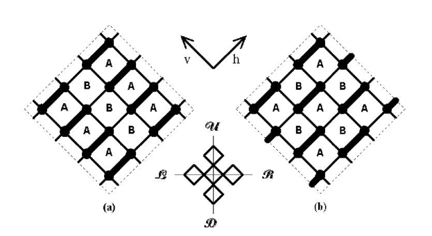
Figure 1: Columnar (a) and staggered (b) states, and the bond (h,v) and the lattice ($\mathcal{R},\mathcal{L},\mathcal{D},\mathcal{U}$) directions.

For the sake of convenience, therefore, we consider a model of classical dimers with solvent on a square lattice, even though other lattices can be considered. The presence of solvent, which can also be treated as void, is not necessary for glass transition as shown recently [10]. Each solvent occupies a site of the lattice. A dimer, on the other hand occupies two consecutive sites and the intervening lattice bond between them. We restrict the excess interaction (energy $\varepsilon)$ to a nearest-neighbor pair of a solvent and an endpoint. It is easy to see that there is no one unique ground state at $T=0.$ Thus, the mere use of the lattice does not produce an ordered structure, which is very comforting for the reasons stated above. To create a unique ground state to mimic a CR, we need to introduce additional interactions between dimers. These are orientational interactions and our model is perfectly suited to investigate the importance of such orientational interactions on the phase diagram. There is an orientational interaction (energy $\varepsilon_{\text{p}})$ between a nearest-neighbor pair of two unbonded dimer endpoints provided the corresponding dimers are parallel. If this interaction is attractive, the ground state at $T=0$ is columnar (Fig. 1a). If the interaction is repulsive, we introduce an additional attractive axial interaction $\varepsilon_{\text{a}}$ between the endpoints of two collinear dimers so that the ground state at $T=0$ is staggered (Fig. 1b). Both ground states have a sublattice structure due to the squares falling into two distinct classes A and B, see Fig. 1. Such ground states also play a central role in the short-ranged resonant valence bond model of high-temperature superconductivity [46], where the pair of parallel dimers (Fig. 1a) are said to resonate; the dimers in Fig. 1b are said to anti-resonate. The dimer interactions are induced by quantum fluctuations. Anderson has hypothesized that the columnar phase with resonating dimers is a good representation of pure La₂CuO₄ which is an insulator.

3.1 Partition Function Formalism

The rigorous thermodynamic treatment of the model is carried out by using the partition function formalism containing the solvent activity $\eta=\exp(\mu/T),$ and the Boltzmann weights $w=\exp(-\varepsilon/T),w_{\text{p}}=\exp(-\varepsilon_{\text{p}}/T)$ and $w_{\text{a}}=\exp(-\varepsilon_{\text{a}}/T).$ We set the Boltzmann constant $k_{\text{B}}=1$. We consider a lattice containing finite and fixed $N_{\text{L}}$ lattice sites. The solvent chemical potential $\mu$ is always kept negative ($\mu<0$) to insure a fully dimer-packed ground state at absolute zero. The configurational PF is given as follows:

$$Z=\sum\Omega(N_{0},N_{\text{p,}}N_{\text{a}},N_{\text{c}})\eta^{N_{0}}w_{\text{p}}^{N_{\text{p}}}w_{\text{a}}^{N\text{a}}w^{N_{\text{c}}},$$ (16)

where $N_{0}$ is the number of the solvent molecules, $N_{\text{p}}$ the number of the nearest-neighbor endpoint contacts between dimers that resonate, $N_{\text{a}}$ the number of nearest-neighbor axial contacts between the endpoints of collinear dimers (pointing in the same direction), $N_{\text{c}}$ the number of nearest-neighbor solvent-endpoint contacts, and $\Omega$ the number of distinct configurations for a given $N_{0},$ $N_{\text{p}}$, $N_{\text{a}},$ and $N_{\text{c}}$. The sum is over $N_{0},$ $N_{\text{p}},$ $N_{\text{a}}$ and $N_{\text{c}}$, consistent with a fixed and finite $N_{\text{L}}$. The densities in the model, to be denoted by $\phi_{k}$, are defined by the limiting ratios $N_{k}/N_{\text{L}}$ per site as $N_{\text{L}}\rightarrow\infty;$ here $k=0,$p,a, and c. The ground state at $T=0$ is determined by whether $\varepsilon_{\text{p}}<0$ (attractive) or $\varepsilon_{\text{p}}>0$ (repulsive). For the attractive case, we set $\varepsilon_{\text{a}}=0$ for simplicity, as its presence does not change the topology of the phase diagram. As shown elsewhere [47], the adimensional free energy

$$\omega=\lim_{N_{\text{L}}\rightarrow\infty}(1/N_{\text{L}})\ln Z$$

represents the osmotic pressure across a membrane permeable to the dimers, but not solvent. The reduced pressure $\pi_{0}\equiv Pv_{0},$ where $v_{0}$ is the volume of a lattice site, is given by

$$\pi_{0}=T\omega-\mu.$$

The equilibrium state must have the highest pressure among all possible states obtained at given $T$, $w_{\text{p}}$, $w_{\text{a}}$ and $\mu$ [47]. The total energy per site $E$ is given by

$$\beta E=-(\phi_{\text{p}}\ln w_{\text{p}}+\phi_{\text{a}}\ln w_{\text{a}}+\phi_{\text{c}}\ln w).$$ (17)

The entropy per site $S$ is calculated through the Legendre transform of the adimensional osmotic pressure:

$$S=\omega+\beta E-\phi_{0}\ln\eta,$$ (18)

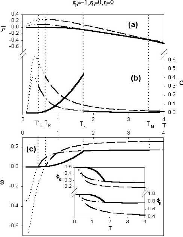
Figure 3: Phase diagram for the case of attractive parallel-dimer interaction and no solvent; temperature dependencies of (a) the shifted thermodynamic potential, (b) the specific heat $C$, (c) the entropy and in the inset of (c) the contact densities $\phi_{\text{a}}$ and $\phi_{\text{p}}$.

where $\phi_{0}$ is the solvent density. Since we are considering a configurational PF, $S$ is purely configurational. (From now on, $S$ and $E$ will represent the configurationl entropy and energy per site and not the entropy and energy of the entire system.) At $T=0$, $\phi_{\text{c}}=0.$ The maximal values of $\phi_{\text{p}},\phi_{\text{a}}$ are easily seen to be 1, and 1/2 (see insets in the Figs. 3c and 7c), respectively. The density $\phi_{\text{e}}$ of nearest-neighbor endpoint pairs due to dimers neither parallel nor collinear has its maximum density 3/2 in the configuration in which dimers form staggered steps. We consider the two cases $\varepsilon_{\text{p}}<0$ (attractive) and $\varepsilon_{\text{p}}>0$ (repulsive) separately. The number of endpoint contacts between resonating dimers is twice the number of resonating dimer pairs. Thus, if $\phi_{\text{RD}}$ denotes the density of pairs of resonating dimers, then $\phi_{\text{RD}}=\phi_{\text{p}}/2.$

4 Husimi Tree Approximation

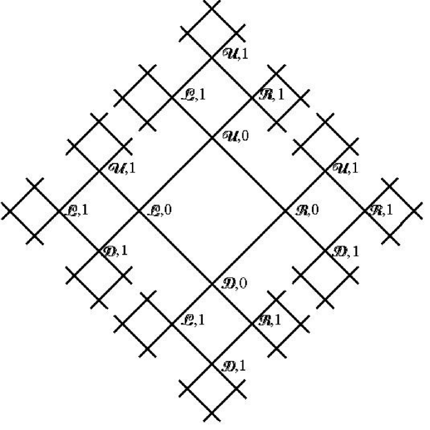
Figure 2: Hisimi tree with labels representing distance from the origin, levels m, and representing orientation with respect to the origin, directional indices $\alpha=\mathcal{R},\mathcal{L},\mathcal{D},\mathcal{U}$.

In order to solve the model exactly, we replace the square lattice by a site-sharing  Husimi cactus shown in Fig. 2, obtained by connecting two squares at each site. This is the only approximation we make. The cactus can be thought of as a checker-board version of the square lattice, representing squares of a given color [9], so that the squares of the other color are missing. However, a pair of dimers on the cactus that would have belonged to a missing square on the original square lattice is counted as a parallel pair on the cactus. Husimi tree incorporates local loop structure of the regular lattice. It is more advantageous than the Bethe lattice as far as the effect of local correlations is concerned, since the Bethe lattice approximation disregards presence of any topological loops. The model is solved exactly on the cactus by recursive technique, which results in RR’s, as shown elsewhere [48]. Because of its exactness, the calculation respects

• all local (such as gauge) and global symmetries, in contrast to the conventional mean-field solution which is known to violate local symmetries, and

• thermodynamics is never violated.

This makes the present approach superior to other methods of constructing mean-field solutions based on random mixing approximation [48], because more local correlations are taken into account. The advantage of using the recursive lattices for the thermodynamic calculations was pointed by Gujrati [48] in connection with a simple trick that allows the calculation of the free energy $\omega$, and various densities exactly.

4.1 Recursion Relations

The lattice sites are indexed by a level index $m$, which increases as we move away from the center of the cactus [8]. If the base site, which is close to the cactus center, of a given square is labeled $m$, then the other three sites of the square (the two intermediate sites connected to the base and the peak site connected to the intermediate sites) are indexed ($m+1$). This square is indexed as $m$th square and is connected to three ($m+1$)th squares. Another index $\alpha$, called the directional index, is introduced to capture the staggered phase on the Husimi tree. We subdivide the lattice sites in four different classes representing the directions on the lattice: up, down, left, and right; see Fig. 1. The squares that lay above their base site are labeled $\mathcal{U}$ (up), below -$\,\mathcal{D}$ (down), to the left - $\mathcal{L}$, and to the right - $\mathcal{R}$ . A square of type $\mathcal{U}$ with its base site at the $m$th level is connected to $\mathcal{L}$, $\mathcal{U}$, and $\mathcal{R}$ (clockwise with respect to the base site) squares with their base sites at the ($m+1$)th level. Similarly, a $\mathcal{D}$ square is connected to the $\mathcal{R}$, $\mathcal{D}$, and $\mathcal{L}$ squares, a $\mathcal{L}$ square is connected to the $\mathcal{D}$, $\mathcal{L}$, and $\mathcal{U}$ squares, and a $\mathcal{R}$ square is connected to the $\mathcal{U}$, $\mathcal{R}$, and $\mathcal{D}$ squares on the upper level. The directional index $\alpha$ of the square will also be associated with its base site. As a convention, the directional index of the peak site of a given square is the same as that of its base site. There are two equivalent ways to view the entire cactus with respect to its origin at $m=0$ [49]. In one view, the origin is taken to be connected to four squares labeled $\mathcal{L}$, $\mathcal{U}$, $\mathcal{R}$, and $\mathcal{D}$, as shown in the Fig. 2. In the other view, the origin is taken to be connected to only two squares labeled $\mathcal{L}$, and $\mathcal{R}$, or $\mathcal{U}$ and $\mathcal{D}$. The former is a symmetric description of the cactus, but more cumbersome, while the latter is an asymmetric description, but easier for calculations. As shown elsewhere [49], both are equivalent in all their consequences.

There are five possible states for a site on the lattice. It is either occupied by a solvent (to be denoted by 0) or by a dimer endpoint with the dimer pointing along one of the four bond directions that we denote by horizontal going up, i.e. pointing away from the origin (h${}_{\text{u}}$), or down, i.e. pointing towards the origin (h${}_{\text{d}}$), and vertical going up or down (v${}_{\text{u}},$v${}_{\text{d}}$); see Fig. 1 for the horizontal (h) and vertical (v) directions. The dimers align themselves on the square lattice in the completely ordered states along a single direction, vertical or horizontal. We introduce the partial partition functions (PPF) $Z_{m}^{(\alpha)}(i)$, given that the site on the level $m$ is in the state $i=0,$h${}_{\text{u}},$h${}_{\text{d}}$,v${}_{\text{u}},$v${}_{\text{d}},$ and has the directional index $\alpha=$ $\mathcal{U}$,$\mathcal{D}$,$\mathcal{L}$,$\mathcal{R}.$ It represents the contribution to the total partition function from the part of the tree above $m$-th level site in the ($i,\alpha$)$-$state. We then obtain the RR’s between $Z_{m}^{(\alpha)}(i)$ at level $m\$and the PPF’s at the higher level $(m+1)$ by considering all possibilities and the local statistical weights of the $(m+1)$th square. In the most general case, the RR’s for the PPF’s are given by a cubic relation for a square Husimi cactus:

$$Z_{m}^{(\alpha)}(i)=\sum w_{jkp}^{(\gamma\delta\alpha)}Z_{m+1}^{(\gamma)}(j)Z_{m+1}^{(\alpha)}(k)Z_{m+1}^{(\delta)}(l),$$ (19)

where ($j,\gamma),$ ($k,\alpha),$ and ($l,\delta$) are the states of the three sites at the level ($m+1)$ (in the clockwise direction from the base site) for each allowed configuration inside the $m$th level polygon and the base site is in the state ($i,\alpha$). The local statistical weight is given by $w_{jkl}^{(\gamma\alpha\delta)}$. The directional indices are $(\gamma\alpha\delta)=(\mathcal{LUR)},(\mathcal{RDL}),(\mathcal{DLU}),$ and $(\mathcal{URD})$ for $\alpha=\mathcal{U},\mathcal{D},\mathcal{L},$and $\mathcal{R},$ respectively. We then use

$$B_{m}^{(\alpha)}\equiv\sum_{i}Z_{m}^{(\alpha)}(i),$$ (20)

in which the sum is over all states $i$, to introduce the ratios

$$x_{i,m}^{(\alpha)}\equiv Z_{m+1}^{(\alpha)}(i)/B_{m+1}^{(\alpha)}.$$ (21)

It is obvious that the ratios always satisfy the sum rule

$$\sum_{i}x_{i,m}^{(\alpha)}=1.$$ (22)

The above RR’s among the partial PF’s is then converted into RR’s relate $x_{i,m}^{(\alpha)}$ with the ratios at the higher level $(m+1)$:

$$x_{i,m}^{(\alpha)}=P_{i,m+1}^{(\alpha)}/Q_{m+1}^{(\alpha)},$$ (23)

where $P_{i,m}^{(\alpha)}$ are various polynomials given by the right-hand side of (19) in which the PPF’s are replaced by the corresponding ratio given in (21) and

$$Q_{m}^{(\alpha)}=\underset{i}{\sum}P_{i,m}^{(\alpha)}.$$ (24)

The explicit expressions for $P_{i,m}^{(\alpha)}$ are given in the Appendix.

4.2 Fix-Point Solutions

The fix-point (FP) solution of the RR’s describe the behavior in the interior of an infinite Husimi cactus. The FP solution can be obtained numerically or analytically (when possible). There are two different kinds of FP solutions. In the 1-cycle FP solution, the ratios remain the same at consecutive levels. We denote the FP values of the ratios by $\{x_{i}^{(\alpha)}\}\equiv\{s^{(\alpha)},h_{\text{u}}^{(\alpha)},h_{\text{d}}^{(\alpha)},v_{\text{u}}^{(\alpha)},v_{\text{d}}^{(\alpha)}\}$. We wish to emphasize that the italicized quantities $h_{\text{u}}^{(\alpha)},$ etc. represent the values of the FP, and should not be confused with the states (h${}_{\text{u}}$,$\alpha$), especially when the description does not require the use of the directional index $\alpha$, which is very much possible as we will see below. The italicized quantities will always represent FP values. In the 2-cycle FP solution, the ratios alternate between two successive levels, which are referred to as even and odd in the following. The ratios on even levels are denoted without prime, and on odd levels with prime. The free energy is calculated using the method originally proposed by Gujrati [48] for the 1-cycle FP and its extension given in [9] for the 2-cycle FP. The FP solution that maximizes the osmotic pressure over a temperature range represents the equilibrium state over that range. This exact solution is taken as the approximate theory for the square lattice. The approach allows us to describe both the ordered, i.e. the crystal (CR) phase at low temperatures and the disordered, i.e. the equilibrium liquid (EL) phase at high temperatures. In addition, an intermediate phase (IP) with intermediate orientational order [more ordered with respect to EL and less ordered with respect to CR] is discovered by the analysis and is involved in a liquid-liquid (L-L) transition induced by orientational interactions; see below for a complete description. True equilibrium states are those that minimize the relevant free energy. Abandoning this minimization principle allows us to obtain metastable states by continuing various solutions [12]. The continuation of EL to lower temperatures describes the supercooled liquid (SCL), which as we show here exhibits the entropy crisis at $T=T_{\text{K}}.$ The disordered liquid EL for the attractive case and SCL for the repulsive case undergo a transition to IP. The continuation of IP to lower temperatures also exhibits an entropy crisis of its own at a temperature $T=T_{\text{K}}^{\prime}$ that is usually different from $T_{\text{K}}$. We study various contact densities in CR, IP and EL, and their continuation. The densities contributing to the energy of different states, upon continuation, approach their corresponding values for CR as $T\rightarrow 0$. Thus, all phases will have identical free energies at $T=0$ if they can exist there. This is consistent with the claim G3 [12]. This equality [8,12] ensures that each of the two metastable states obtained by continuing EL and IP will exhibit entropy crisis.

5 Results

We consider the cases $\eta=0$, and $\eta>0$, separately as we are able to obtain analytical solutions for the former case. For the case $\eta=0$, $\omega$ is related to the Helmholtz free energy $F(T)$: $F(T)=-T\omega$ [8]. For $\eta>0,$ $\pi_{0}$ is related to the thermodynamic potential $F(T)=-\pi_{0}.$ To cover both cases together we define the following shifted thermodynamic potential $\overline{F}$:

$$\overline{F}(T)\equiv F(T)-F(0)=-T\omega-E_{0},$$

where $E_{0}$ is the energy of the perfect CR at $T=0$. It has the property that it vanishes at $T=0$. The vanishing of entropy corresponds to the maximum in $\overline{F}(T).$

5.1 Disordered Phase: EL and SCL

The disordered phase is the continuation of the phase at infinite temperatures, where the correlations are minimal. This phase is described by a 1-cycle FP solution.

5.1.1 Absence of Solvent

We study both attractive and repulsive cases together. The relevant FP solution corresponds to having complete equivalence among all quantities with different directional indices. Thus, we will suppress the directional index $\alpha$ ($x_{i}^{(\mathcal{R})}$ = $x_{i}^{(\mathcal{L})}$ = $x_{i}^{(\mathcal{D})}$ = $x_{i}^{(\mathcal{U})}\equiv x_{i}$) at present. The RR’s for such a FP solution are the following:

$$Qh_{\text{d}}\text{{}} =\text{(}w_{\text{a}}w_{\text{p}}\text{)}^{2}h_{\text{u}}^{3}+3w_{\text{a}}w_{\text{p}}h_{\text{u}}^{2}v_{\text{u}}+(1+2w_{\text{a}}w_{\text{p}})v_{\text{u}}^{2}h_{\text{u}}$$ (25)

$$+w_{\text{a}}w_{\text{p}}v_{\text{u}}^{3}+w_{\text{a}}h_{\text{d}}^{2}h_{\text{u}}+h_{\text{d}}^{2}v_{\text{u}}+w_{\text{p}}h_{\text{u}}v_{\text{d}}^{2}+v_{\text{u}}v_{\text{d}}^{2},$$

$$Qv_{\text{d}} =w_{\text{a}}w_{\text{p}}h_{\text{u}}^{3}+3w_{\text{a}}w_{\text{p}}v_{\text{u}}^{2}h_{\text{u}}+(1+2w_{\text{a}}w_{\text{p}})h_{\text{u}}^{2}v_{\text{u}}$$

$$+(w_{\text{a}}w_{\text{p}})^{2}v_{\text{u}}^{3}+h_{\text{d}}^{2}h_{\text{u}}+w_{\text{p}}h_{\text{d}}^{2}v_{\text{u}}+h_{\text{u}}v_{\text{d}}^{2}+w_{\text{a}}v_{\text{u}}v_{\text{d}}^{2},$$

$$Qv_{\text{u}} =v_{\text{d}}(w_{\text{p}}h_{\text{u}}^{2}+2v_{\text{u}}h_{\text{u}}+w_{\text{a}}v_{\text{u}}^{2}+w_{\text{p}}^{2}v_{\text{d}}^{2}),$$

$$Qh_{\text{u}} =h_{\text{d}}(w_{\text{p}}v_{\text{u}}^{2}+2v_{\text{u}}h_{\text{u}}+w_{\text{a}}h_{\text{u}}^{2}+w_{\text{p}}^{2}h_{\text{d}}^{2}).$$

The polynomial $Q,$ see (24), is given by the sum of the right-hand sides in the above equation because of the sum rule (22) for the ratios, where we must recognize that $s$ is zero because of $\eta=0.$

The osmotic pressure for this solution is calculated from general expressions, which follows from the Gujrati trick [48]. The central square is conneted to 4 branches extending in different directions. Recalling that the index $\alpha$ is suppressed in the quantity $B_{m}^{(\alpha)},$ we find that the total PF of the entire lattice is given by

$$Z_{0}=B_{0}^{4}QQ_{0},$$

where

$$Q_{0}=2v_{\text{u}}v_{\text{d}}+2h_{\text{u}}h_{\text{d}}+s^{2}/\eta.$$

We now imagine taking out the 5 squares at the origin, which leaves behind 9 smaller branches of the cactus, from which we construct 3 smaller lattices by connecting 4 branches together each. The total PF of each of the smaller lattices is given by

$$Z_{1}=B_{1}^{4}QQ_{0},$$

so that [48]

$$\omega=(1/4)\ln(Z_{0}/Z_{1}^{3}).$$

Since $B_{0}=B_{1}^{3}Q,$ see (20) and (21), we finally have

$$\omega=(1/2)\ln\left(Q/Q_{0}\right).$$

We can also calculate the densities of various types of contacts. For this, we consider the single square at the origin and consider all of their possibilities that contribute to the quantities of interest. Dividing this contribution with the total PF $Z_{0}$ yields the density per site as $\phi_{\lambda}=\Phi_{\lambda}/QQ_{0},$ $\lambda=$p,a, where

$$\Phi_{\text{p}} =w_{\text{p}}(2w_{\text{a}}h_{\text{u}}^{2}v_{\text{u}}^{2}+v_{\text{d}}^{2}h_{\text{u}}^{2}+h_{\text{d}}^{2}v_{\text{u}}^{2}+2w_{\text{a}}v_{\text{u}}^{3}h_{\text{u}}+2w_{\text{a}}v_{\text{u}}h_{\text{u}}^{3})$$ (26)

$$+w_{\text{p}}^{2}(w_{\text{a}}^{2}v_{\text{u}}^{4}+w_{\text{a}}^{2}h_{\text{u}}^{4}+h_{\text{d}}^{4}+v_{\text{d}}^{4}),$$

$$\Phi_{\text{a}} =w_{\text{a}}(2w_{\text{p}}v_{\text{u}}h_{\text{u}}^{3}+v_{\text{d}}^{2}v_{\text{u}}^{2}+2w_{\text{p}}v_{\text{u}}^{3}h_{\text{u}}+2w_{\text{p}}v_{\text{u}}^{2}h_{\text{u}}^{2}+h_{\text{d}}^{2}h_{\text{u}}^{2})+$$ (27)

$$+(w_{\text{a}}w_{\text{p}})^{2}(h_{\text{u}}^{4}+v_{\text{u}}^{4}).$$

There is an additional symmetry in the FP solution of interest for the disordered phase. This symmetry corresponds to having

$$h_{\text{u}} =v_{\text{u}}\equiv a,$$ (28)

$$h_{\text{d}} =v_{\text{d}}\equiv b.$$

The resulting system of FP equations are

$$b =\left(a^{3}K_{1}+ab^{2}K_{2}\right)/Q,$$

$$a =\left(ba^{2}K_{2}+b^{3}w_{\text{p}}^{2}\right)/Q,$$

$$Q =2\left(a^{3}K_{1}+ab^{2}K_{2}+ba^{2}K_{2}+b^{3}w_{\text{p}}^{2}\right),$$

where

$$K_{1} =(w_{\text{a}}w_{\text{p}})^{2}+6(w_{\text{a}}w_{\text{p}})+1,$$

$$K_{2} =w_{\text{a}}+w_{\text{p}}+2,$$

can be solved analytically making the substitution $r=b/a$:

$$r=(K_{1}/w_{\text{p}}^{2})^{1/4}.$$ (29)

Using the sum rule $2a+2b=1,$ which follows from (22), we eventually have

$$Q^{\text{dis}} =ab(K_{2}+\sqrt{K_{1}w_{\text{p}}^{2}}),$$

$$Q_{0}^{\text{dis}} =4ab.$$

We finally find for the disordered phase

$$\omega^{\text{dis}} =\frac{1}{2}\ln\left(K_{2}+\sqrt{K_{1}w_{\text{p}}^{2}}\right)-\ln 2,$$ (30)

$$\phi_{\text{p}}^{\text{dis}} =\frac{3w_{\text{p}}w_{\text{a}}+w_{\text{p}}r^{2}+2(w_{\text{p}}w_{\text{a}})^{2}+2w_{\text{p}}^{2}r^{4}}{2r^{2}(K_{2}+\sqrt{K_{1}w_{\text{p}}^{2}})},$$

$$\phi_{\text{a}}^{\text{dis}} =\frac{3w_{\text{a}}w_{\text{p}}+w_{\text{a}}r^{2}+(w_{\text{a}}w_{\text{p}})^{2}}{2r^{2}(K_{2}+\sqrt{K_{1}w_{\text{p}}^{2}})},$$

$$S_{\text{dis}} =\omega^{\text{dis}}-\phi_{\text{p}}^{\text{dis}}\ln w_{\text{p}}-\phi_{\text{a}}^{\text{dis}}\ln w_{\text{a}}.$$

The solution described above represents the equilibrium state at high temperatures. Thus, we identify it as the disordered liquid phase stable at high temperatures, see below for a complete description.

At this point we refer to the famous calculations by Kasteleyn [50] and by Fisher [51] who provided the exact value for the number of fully-packed dimer packings (no solvent) on a square lattice, $\varphi_{\text{exact}}=1.7916$ where $\varphi$ is the molecular freedom per site, $\varphi=\exp(2S)$. The high-temperature limit of $S_{\text{dis}}$ in (30) represents the number of configurations for weakly interacting dimers on Husimi cactus. Taking the limit $w_{\text{a}}\rightarrow 1,$ $w_{\text{p}}\rightarrow 1$ we find $\varphi_{\text{Husimi}}=1.7071.$ To appreciate the improvement due to the use of the Husimi cactus over the Bethe lattice we compare this with $\varphi_{\text{Bethe}}=1.6875$ obtained by Chang [52].

5.1.2 Presence of Solvent

We investigate the effect of solvent by letting $\eta\neq 0.$ We now consider nearest-neighbor solvent -dimer end-point interactions, which we take not do depend on the dimer orientation. These are ordinary isotropic interactions with energy given by the standard exchange or excess expression: $\varepsilon=e_{0\text{m}}-1/2(e_{00}+e_{\text{mm}})=-1/2e_{\text{mm}}$, where $e_{0\text{m}},$ $e_{00}$, and $e_{\text{mm}}$ are direct solvent-monomer, solvent-solvent, and monomer-monomer interaction energies [45]. Apart from $\varepsilon$, we have the chemical potential $\mu$ to control the amount of solvent particles in the system. We are no longer able to find the FP solution analytically, and are forced to use numerical methods to find it. The presence of solvent modifies the RR’s in (25), since we need to also incorporate the state $i=0$ describing the solvent presence at each level. The general RR’s in the Appendix can be used to construct the 1-cycle RR’s. The results of this numerical solution is presented below when we discuss the entire phase diagram.

5.2 Ordered Phases CR and IP in the Attractive Case

In case when parallel-dimer configurations become more favorable as $T\rightarrow 0,$ the ground state is the columnar phase. There is no need for the axial interactions to attain the complete order at $T=0$; therefore first we set $\varepsilon_{\text{a}}=0$, and consider the effect of $\varepsilon_{\text{a}}<0$ later. Attractive axial interaction only enhances the chance of forming the ordered state. The symmetry of the ground state does not require using directional indices thereby simplifying our RR’s. In addition to the disordered equilibrium liquid EL discussed above and stable at high temperatures, our solution captures two ordered phases: columnar state CR, which is the equilibrium state at low temperatures, and a phase IP with an intermediate order, which is the equilibrium state at intermediate temperatures before EL becomes the equilibrium state.

5.2.1 Absence of Solvent

At first, we study the pure dimer system with $\eta=0$. Three phases are distinguished by the symmetries of their FP structures. The EL solution was already described in previous section, where it was found that $h\equiv h_{\text{u}}+h_{\text{d}}$ $=$ $v\equiv v_{\text{u}}+v_{\text{d}}=a+b=1/2$ - the numbers of vertical and horizontal dimers are the same. The perfect columnar CR ($T=0$) on the cactus has each A square surrounded by B squares, and vice versa - consider the checker-board version of the A-B sublattice structure for squares in Fig. 1a. This property is captured by applying a 2-cycle scheme when the FP conditions for even and odd lattice sites are attained separately. We take the convention that even (odd) squares on the Husimi tree have even (odd) base sites. In the case when the dimers in the perfect CR occupy even squares and are oriented in the horizontal direction (horizontally resonating dimers), we have $h_{\text{u}}=1$, $v_{\text{u}}=0,$ $h_{\text{d}}^{\prime}=1,$ $v_{\text{d}}^{\prime}=0$. The perfect CR with dimers resonating vertically $(v_{\text{u}}=1$, $h_{\text{u}}=0,$ $v_{\text{d}}^{\prime}=1,$ $h_{\text{d}}^{\prime}=0)$ or resonating dimers occupying odd polygons are disjoint from the above horizontally resonating CR phase and does not have to be considered separately. As the temperature is raised, CR begins to distort such that $h_{\text{u}},$ and $h_{\text{d}}^{\prime}$ decrease and $v_{\text{u}},$ and $v_{\text{d}}^{\prime}$ increase. On the other hand, IP is given by a solution which satisfies $h_{\text{u}}=$ $v_{\text{u}}=$ $h_{\text{d}}^{\prime}=$ $v_{\text{d}}^{\prime}=1/2$ and which is independent of temperature. The 2-cycle structure of the solution suggests that dimers continue to resonate locally occupying even squares, but resonating pairs on average have no preference whether to orient horizontally or vertically. Therefore, we can say that the IP is characterized by the positional order but no orientational order, which is the general definition of a plastic crystal.

The perfect CR that has $T\omega^{\text{ord}}=-\varepsilon_{\text{p}}$, $S_{\text{ord}}=0$, $\phi_{\text{p}}^{\text{ord}}=1$, $\phi_{\text{a}}^{\text{ord}}=1/2$ is thermodynamically stable at temperatures close to zero as expected. In the following we assume that all dimers are horizontal. As the CR heats up, resonating dimer pairs begin to resonate in the vertical direction maintaining their positions within even squares with the result that $S_{\text{ord}}$ increases, and $\phi_{\text{p}}^{\text{ord}}$ and $\phi_{\text{a}}^{\text{ord}}$ decrease. At some point, CR undergoes a continuous transition and a new state IP appears; the transition point is shown in Fig. 3 at $T_{\text{c}}\cong 1.7$. In IP, the densities of resonating dimers in the two directions remain equal to each other. The density of endpoint contacts due to dimers resonating within A (or B) squares only $\phi_{\text{p,res}}^{\text{IP}}=1/2$ remains independent of the temperature, while $\phi_{\text{p}}^{\text{IP}}$ continues to decrease slowly. We also have ($K_{1}=1+6w_{p}+w_{p}^{2})$

$$\phi_{\text{a}}^{\text{IP}}=(3w_{\text{p}}+w_{\text{p}}^{2})/2K_{1},\text{ \ \ }\phi_{\text{p}}^{\text{IP}}=1/2+\phi_{\text{a}}^{\text{IP}},$$

$$\omega^{\text{IP}}=(1/4)\ln\left(K_{1}w_{\text{p}}^{2}/4\right).$$

Figure 3 shows the equilibrium states by solid lines, EL-metastable extension SCL at lower temperatures by the dashed line, IP-metastable extensions at higher and lower temperatures by dash-dotted lines. The equilibrium status is resolved by comparing the free energy $F(T)=-T\omega$ for all solutions obtained at a given temperature as shown in Fig. 3a. We also present the specific heat curves, $C$, in the same figure but using the right axis. Figure 3c shows the configurational entropy, and the contact densities $\phi_{\text{a}}$ and $\phi_{\text{p}}$ are given in the inset. Note that the configurational entropy becomes zero at the point where $F(T)$ is maximum. Below the maximum, the entropy becomes negative and, therefore, this portion of the extension cannot represent any realizable state. The extensions are shown by dotted lines. Thus, the maximum in $F(T)$ locates the Kauzmann temperature. This is our main result. We also note that both SCL and the supercooled IP states exhibit the entropy crisis. The solutions are obtained below correspond to negative entropies According to ideas traced back to times of entropy crisis discovery [1,16], a metastable curve must be terminated at its Kauzmann point where the system undergoes an ideal glass transition, the ideal glass being a frozen and unique disordered structure. Note that the transition is not dictated by the statistical mechanical treatment, but by an additional requirement that the configurational entropy be non-negative; see G4 above. The emergence of an ideal glass cannot be verified experimentally due to tremendous slowing down below the experimentally observed glass transition. We emphasize here that the above entropy crisis has been demonstrated for the first time in an explicit calculation for a model of molecular liquid.

The EL undergoes a first-order transition to IP at the melting temperature, $T_{\text{M}}\cong 3.6$ in Fig. 3. The continuation of EL below $T_{\text{M}}$ gives rise to SCL, whose entropy vanishes near $T_{\text{K}}\cong 0.64,$ thus establishing the existence of an entropy crisis in small molecules. Similarly, the continuation of IP below $T_{\text{c}}$ describes its metastable state whose entropy also vanishes near $T_{\text{K}}^{{}^{\prime}}\cong 0.44$, thus giving rise to another entropy crisis. Our exact calculation also shows that the contact densities of both metastable states approach the values for the ideal crystal as $T\rightarrow 0$, namely $\phi_{\text{a}}^{\kappa}\rightarrow 1/2$, $\phi_{\text{p}}^{\kappa}\rightarrow 1$, where $\kappa=$ dis, IP, and CR. Equality of $\phi_{\text{p}}^{\kappa}$ is consistent with the energy equality at $T=0;$ see G3 above. The equality of $\phi_{\text{a}}^{\kappa}$ is due to the fact that it is determined uniquely by $\phi_{\text{p}}^{\kappa}$ at $T=0$. The entropies of the metastable branches approach negative values at $T=0$: $S_{\text{IP}}\rightarrow-\ln\sqrt{2}$, and $S_{{}^{\text{dis}}}\rightarrow-\ln 2$.

The differences between the three phases in the attractive case can be summarized as below. Let $h\equiv h_{\text{u}}+h_{\text{d}},=$ and $v\equiv v_{\text{u}}+v_{\text{d}}$ at each level, whether even or odd. (For odd levels, we have primed quantities$.)$ The calculation shows that

• EL has the 1-cycle structure and has $h=v$ at each level.

• IP has the 2-cycle structure but still has $h=v$ at each level.

• CR has the 2-cycle structure but does not satisfy $h=v$ at each level.

5.2.2 Presence of Solvent

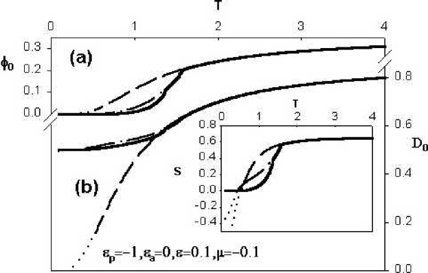
Figure 4: Illustration of the effect of free volume for $\varepsilon_{\text{p}}<0,\varepsilon_{\text{a}}=0$. Temperature dependencies of (a) the free volume, (b) the ratio $D_{0}=\phi_{00}/\phi_{0}$, and the entropy in the inset.

The presence of solvent eventually makes melting transition to become second-order. Figure 4 includes the curves for a typical solvent density dependence shown by the upper curves, and the ratio of the density of solvent-solvent contacts to the solvent density,

$$D_{0}\equiv\phi_{00}/\phi_{0},$$

shwon by the lower curves. The inset shows the entropy curve for this case. The ratio $D_{0}\equiv N_{00}/N_{0}$ representing the number of solvent-solvent contacts per solvent is a measure of solvent localization in analogy with holon localization in the quantum dimer model. If the solvent particles were randomly distributed, then $\phi_{00}=2\phi_{0}^{2},$ so that $D_{0}=2\phi_{0}.$ If the solvent particles were paired as two nearest-neighbor solvent particles (dimerized solvent) so as to replace a dimer, then $\phi_{00}=\phi_{0}/2$, and $D_{0}=1/2.$ If the solvent particles appear as a cluster of four to replace two dimers inside a square, then $D_{0}=1,$ and so on. Thus, $\phi_{00}/\phi_{0}$ provides us with the information about the nature of their distribution. We expect the random distribution at very high temperratures. From Fig. 4, we see that $D_{0}$ is sligfhtly larger than $\phi_{0}$ at higher temperaturers, implying that the solvent distribution is still highly correlated. At low temperatures, we find that $D_{0}^{\text{CR}}=D_{0}^{\text{IP}}=1/2$, indicating that solvents appear in the form of a dimerized solvent to replace a single dimer. In contrast, $D_{0}^{\text{SCL}}$ approaches zero, implying that the solvents are not dimerized in it. This is an interesting observation in view of the fact that all have vanishingly small solvent density near absolute zero. At higher temperatures, $\phi_{0}^{\text{SCL}}$ is much higher than $\phi_{0}^{\text{CR}}$ and $\phi_{0}^{\text{IP}}.$

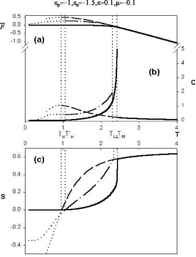
Figure 5: Plot demostrating the effect of attractive axial interaction for $\varepsilon_{p}<0$. Increasing the strength of the attractive axial interaction makes IP to apperar in the SCL region.

Introducing attractive axial interactions makes CR to be stable at higher temperatures, thus destroying IP. The higher the strength of the attractive axial interactions, the larger $\left|\varepsilon_{\text{a}}\right|,$ the higher $T_{\text{c}}$ moves. Large enough $\left|\varepsilon_{\text{a}}\right|$ destroys the stable portion of IP resulting in second-order liquid-liquid transition to occur in SCL region, see Fig. 5. Once $\varepsilon$ and $\mu$ are kept constant, increasing $\left|\varepsilon_{\text{p}}\right|$ results in higher melting and Kauzmann temperatures and larger free volume densities.

5.3 Ordered Phases CR and IP in the Repulsive Case ($\varepsilon_{\text{p}}>0)$

5.3.1 Absence of Solvent

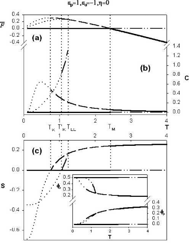
Figure 6: Phase diagram for the case of repulsive parallel-dimer interaction and no solvent. The liquid-liquid transition at $T_{\text{LL}}$ is below the melting point at $T_{\text{M}}$.

The staggered ground state (Fig. 1b) with all dimers aligned in one direction, taken to be horizontal in Fig. 1b, is achieved only when, in addition to the repulsive parallel-dimer interaction, an attractive axial interaction is introduced. Moreover, the staggered state requires a different description than the one used to describe the columnar phase studied above. This is clear from the fact that the ground state on the cactus (consider the checker-board version of Fig. 1b) either contains either A squares or B squares. The two intermediate sites in a given square on the cactus are in different states (the bond goes up or to down), but the upper and the base lattice sites are in the same state. In order to capture this particular property of the ground state, we need to distinguish the four sites by their color index $\alpha=$ $\mathcal{U}$,$\mathcal{D}$,$\mathcal{R}$,$\mathcal{L}$. As in the previous case, three types of FP solutions of different symmetries are obtained: the disordered liquid EL discussed earlier, the crystal (CR), and the intermediate phase (IP). The situation is depicted in the Figs. 6a,b. The solid curves represent the equilibrium states EL and CR, with a discontinuous transition between them at the melting point $T_{\text{M}}$. We also show their metastable extensions depicted by dashed (SCL) and dash-dot-dot (superheated CR) curves. A liquid-liquid continuous transition occurs at $T_{\text{LL}}$ between SCL and IP. The later is shown by the dash-dot curve, which originates at $T_{\text{LL}}$ and continues all the way down to absolute zero, just like SCL. It is clear from Fig. 6b that both SCL and IP exhibit the entropy crisis at $T_{\text{K}}$ and $T_{\text{K}}^{{}^{\prime}}.$ We show their extensions below their respective Kauzmann temperatures by dotted curves.

The equilibrium state EL at high temperatures has been described above where the index $\alpha$ was omitted. Our numerical solution for the system of 1-cycle RR’s that result when $\alpha$ is taken into account predicts the same free energy and densities as given by equations (30). However the new solutions have a slightly different symmetry ($x_{i}^{(\mathcal{U})}=x_{i}^{(\mathcal{D})}$), ($x_{i}^{(\mathcal{L})}=x_{i}^{(\mathcal{R})}$) whereas the earlier EL solution requires the symmetry ($x_{i}^{(\mathcal{U})}=x_{i}^{(\mathcal{D})})=(x_{i}^{(\mathcal{L})}=x_{i}^{(\mathcal{R})}$). (The latter symmetry can be obtained by an appropriate choice of the intitial guesses for the new RR’s.) In addition the solution also has the following symmetry: $h^{(\alpha)}\equiv$ $h_{\text{u}}^{(\alpha)}+$ $h_{\text{d}}^{(\alpha)}$ $=$ $v^{(\alpha)}\equiv$ $v_{\text{u}}^{(\alpha)}+$ $v_{\text{d}}^{(\alpha)}$. The symmetry of IP is somewhat similar to that of EL. It is also obtained in 1-cycle scheme and has the partial symmetry $x_{i}^{(\mathcal{U})}=x_{i}^{(\mathcal{D})},$ $x_{i}^{(\mathcal{L})}=x_{i}^{(\mathcal{R})}$, but $h^{(\alpha)}\neq$ $v^{(\alpha)}$.

There four possible 1-cycle solutions representing four disconnected CR states at $T=0$ are the following.

$$\{h_{\text{d}}^{(\mathcal{R}\text{)}} =h_{\text{u}}^{(\mathcal{L}\text{)}}=h_{\text{d}}^{(\mathcal{D}\text{)}}=h_{\text{u}}^{(\mathcal{U}\text{)}}=1\}\text{ or}$$ (31)

$$\{h_{\text{u}}^{(\mathcal{R}\text{)}} =h_{\text{d}}^{(\mathcal{L}\text{)}}=h_{\text{u}}^{(\mathcal{D}\text{)}}=h_{\text{d}}^{(\mathcal{U}\text{)}}=1\}\text{ or}$$

$$\{v_{\text{d}}^{(\mathcal{R}\text{)}} =v_{\text{u}}^{(\mathcal{L}\text{)}}=v_{\text{u}}^{(\mathcal{D}\text{)}}=v_{\text{d}}^{(\mathcal{U}\text{)}}=1\}\text{ or}$$

$$\{v_{\text{u}}^{(\mathcal{R}\text{)}} =v_{\text{d}}^{(\mathcal{L}\text{)}}=v_{\text{d}}^{(\mathcal{D}\text{)}}=v_{\text{u}}^{(\mathcal{U}\text{)}}=1\}.$$

Only one out of the above four CR states will occur due to symmetry breaking.

The staggered phase is an example of a frozen state, which does not allow creating any local imperfections when voids are forbidden. Once trapped in it at low $T$, the system remains frozen in a single microstate as the temperature is elevated further. This is signified by the temperature-independent osmotic pressure; hence, the solution for CR is temperature-independent. Consequently, the CR entropy $S_{\text{ord}}=0$. In addition, $\phi_{\text{a}}^{\text{ord}}=1/2$ and $\phi_{\text{p}}^{\text{ord}}=0$ remain constant. As expected, CR is the equilibrium state at low temperatures, while EL is the equilibrium state at high temperatures. The melting transition between these two states takes place at $T_{\text{M}}\cong 3.6$ where densities change discontinuously. Both CR and EL have their extensions into the metastable region shown by means of dashed curves. The EL extension below $T_{\text{M}}$ yields SCL. Another metastable liquid phase IP is found in the SCL region where it meets continuously with SCL via a second-order liquid-liquid transition at $T_{\text{LL}}\cong 2.5.$ The new phase IP has much higher $\phi_{\text{a}}$ and lower $\phi_{\text{p}}$ relative to SCL so that the dimers are preferentially oriented in one direction in IP. The specific heat curves for SCL and IP show relatively large discontinuity at $T_{\text{LL}}$.

Both SCL and IP exhibit their own entropy crises at different temperatures, $T_{\text{K}}\cong 1.1$ and $T_{\text{K}}^{{}^{\prime}}\cong 1.7$ respectively. Although they are not absolutely stable compared to CR, the free energy $\omega^{\text{IP}}$ of the IP is higher than that of SCL. The calculation predicts negative configurational entropies for the extensions of SCL and IP below their Kauzmann temperatures represented by dotted curves in Fig. 6b. The density values for the extensions of EL and IP reach the crystalline values at $T=0$ so that SCL, IP, and CR have the same energy $E_{0}=\varepsilon_{\text{a}}/2;$ see G4 above. Thus, our exact calculations confirms the theorem of identical energies of all possible stationary states proven in [12]. We also find that the entropies of SCL and IP are extrapolated to $-\ln 2$ and $-\ln\sqrt{2}$ respectively at $T=0$, so that $TS\rightarrow 0$ as $T\rightarrow 0$, a condition for the identical energy theorem.

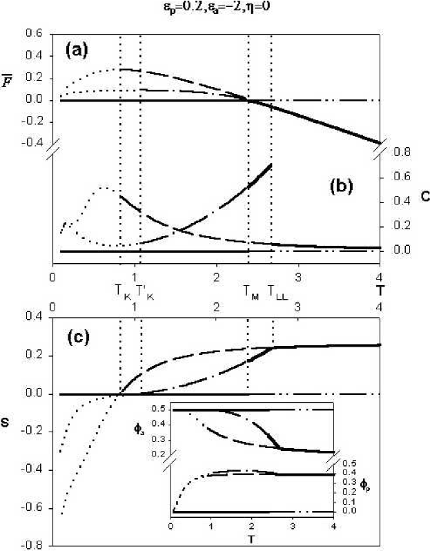
Figure 7: Phase for the repulsive parallel-dimer interaction representing the liquid-liquid transition above the melting point.

Changing $\varepsilon_{\text{p}}$ affects $T_{\text{M}}$ much stronger than $T_{\text{LL}},$ vis. $T_{\text{M}}$ decreases with reduction of $\varepsilon_{\text{p}}$. Figure 7 demonstrates the situation when $T_{\text{LL}}\cong 2.6$ is moved above $T_{\text{M}}\cong 2.4$. We also have $T_{\text{K}}\cong 0.83$ and $T_{\text{K}}^{\prime}\cong 1.1$.

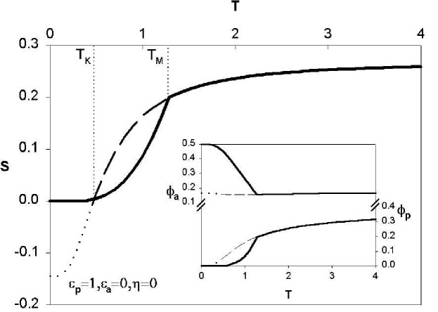
Figure 8: Phase diagram for the case as the strength of the axial interaction is tending to zero.

The liquid-liquid transition temperature moves towards the melting temperature as the strength $\left|\varepsilon_{\text{a}}\right|$ of the attractive axial interactions increases. At the same time, the melting temperature rises with $\left|\varepsilon_{\text{a}}\right|$. Reducing axial attraction eventually makes IP to appear below $T_{\text{K}}$ only. Thus, IP is induced by axial interactions. In the limit when $\left|\varepsilon_{\text{a}}\right|\rightarrow 0,$ IP disappears from the phase diagram completely, see Fig. 8. The inset shows that we capture the crystalline state that has $\phi_{\text{a}}^{\text{ord}}=1/2$ at $T=0$, while $\phi_{\text{a}}^{\text{SCL}}$ approaches to $1/6$ at $T=0$.

The differences between the three phases in the repulsive case can be summarized as below. The calculation shows that

• EL has the property $h=v$ at each level for each direction $\alpha$, and individual $x_{i}^{(\mathcal{U})}=x_{i}^{(\mathcal{D})},$ and $x_{i}^{(\mathcal{L})}=x_{i}^{(\mathcal{R})}$.

• IP does not have the property h=v at each level for each direction $\alpha$, but still has $x_{i}^{(\mathcal{U})}=x_{i}^{(\mathcal{D})},$ and $x_{i}^{(\mathcal{L})}=x_{i}^{(\mathcal{R})}$.

• CR has neither of the properties of EL.

5.3.2 Presence of Solvent

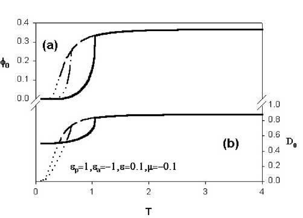
Figure 9: Temperature dependencies of (a) the free volume and (b) the ratio $D_{0}=\phi_{00}/\phi_{0}$ for the case of repulsive parallel-dimer interaction.

The crystalline state is no longer frozen when the solvent is introduced. As we increase $\mu$ and decrease $\varepsilon,$ the discontinuities in densities at $T_{\text{M}}$ become smaller and smaller. Eventually melting transforms into a second-order transition. The presence of the solvent makes $T_{\text{M}}$ go down; The larger $\mu$ and the smaller $\varepsilon$ are, the smaller $T_{\text{M}}$ becomes. Figure 9 shows the solvent density $\phi_{0}$. Compared to the case of $\varepsilon_{\text{p}}<0,$ the values of $\phi_{0}$ at the Kauzmann temperatures are much larger. The solvent density in SCL is larger than in IP and the same holds for the ratio $D_{0}.$ From Fig. 9, we immediately note that the relative amount of dimerized solvents is higher in SCL than in IP for this case.

6 Discussion and Conclusions

We have argued that the configurational entropy is the central concept and has to be defined properly if we have any chance of success in explaining the experimentally observed glass transition in supercooled viscous liquids. We have followed the conventional definition of the configurational entropy, which is obtained by considering the configurational degrees of freedom and is obtained by subtracting the entropy $S_{\text{KE}}(T)$ due to the translational degrees of freedom from the total entropy. It is this configurational entropy that is used to define the configurational partition function. This definition is compared with other definitions of configurational entropy used by experimentalists and have shown that their definitions are operational in spirit to estimate the configurational entropy since the latter is not experimentally accessible, at least at present by any known technique.

Following the original suggestion of Kauzmann, we have adopted the view that observing $S_{\text{SCL}}<0$ under extrapolation of experimental values of $S_{\text{SCL}}$ implies that such extrapolated states cannot exist. Any state to be observed in Nature must, as a prerequisite, have a non-negative entropy. This principle must be obeyed by any observed state in Nature, regardless of whether the state is an equilibrium state, a strongly time-dependent metastable state, or a stationary metastable state. We have shown that while it is possible in theoretical investigations to probe the stationary limit of SCL or other metastable states and be able to investigate the ideal glass transition, which is invoked to avoid the configurational entropy crisis ($S_{\text{SCL}}<0$), it is impossible to establish the existence of the ideal glass transition without the help of extrapolation in experiments or numerical simulation, since they only deal with states that exist in Nature. Consequently, they will only access states for which the configurational entropy must strictly be non-negative.

Since the value of the configurational entropy is crucial in locating the Kauzmann temperature, we have shown how to define the entropy properly ($S\geq 0$) by discretizing the real and momentum spaces. This procedure ensures $S\geq 0.$ We then argue that since the translational degrees of freedom are decoupled from the configurational degrees of freedom, we need to ensure the non-negativity of each of the entropy from the two degrees of freedom. Since the entropy due to the kinetic energy is always non-negative, we need to only verify whether the configurational entropy is non-negative so that the entropy crisis would not occur.

One of the major aims of the work was to establish the existence of the entropy crisis in metastable molecular fluids. We have developed a simple model of molecular fluids composed of dimers. The model is defined on a lattice so that it only contains configurational entropy and contains directional and direction-independent interactions. One of the former interactions is the interaction between the end-points of the dimers, which is either attractive or repulsive, and is used to broadly classify the molecular liquid into attractive and repulsive cases. This is because the CR-symmetry in the two cases are very different, as shown in Fig. 1.

The model is solved exactly on a special kind of recursive lattices, commonly known as the site-sharing Husimi cactus. The cactus is an approximation of a square lattice and shares with it the coordination number and the smallest loop size. The method of solution uses recursive technique, which is standard by now. What distinguishes the present analysis with most other similar investigations is that the ordered phase (CR and IP) descriptions require identifying novel FP structures with appropriate symmetries, which are very different from the symmetry of the FP solution describing the disordered phase (EL and its metastable extension SCL). This also requires us to calculate the osmotic pressure ($\eta>0$) or the free energy ($\eta=0$) appropriately.

Because of the directional interactions, we also obtain an intermediate phase IP, which may or may not be an equilibrium state depending on the directional interactions. In the attractive case, IP is an equilibrium state, but its extension at low temperatures is a metastable state with respect to CR. However, for the repulsive case, it is a metastable state in Fig. 5 and an equilibrium state in Fig. 6. In both cases, its extension at low temperatures is a metastable state with respect to CR. Both EL and IP have their extensions that exhibit their own entropy crisis. The fact that EL’s metastable extension SCL exhibits an entropy crisis is not a surprise on its own, since this is what we intended to demonstrate, it came as a surprise that the metastable extension of IP (which itself may be a metastable state with respect to CR, but an ”equilibrium state” with respect to SCL) also exhibited a Kauzmann temperature of its own. This is consistent with the rigorous analysis of Gujrati [12], which demonstrates the existence of an entropy crisis in a state which is a metastable extension with respect to CR. The argument is applicable to any number of metastable extensions, as long as these extensions are of stationary nature.

The model is rich enough due to its complex energetics that we also find liquid-liquid transition in the model. The transition is driven by the directional interactions in the model. The distributions of solvent particles in the metastable states are very different from that in CR. This is seen clearly from the behavior of $D_{0}.$

The analysis of the present work also confirms the equal energy principle G3 at $T=0$ for all states that can be continued to $T=0$; here, we are carrying out the continuation without any regard to the principle of reality ($S\geq 0$). This is important as it immediately implies that there must be a positive Kauzmann temperature. We further note that $TS(T)\rightarrow 0$ for all of the states. This condition is a prerequisite for the Gujrati proof [12].

Because of  the equal energy observation, the question that naturally arises is whether all the states at absolute zeo represent the same state. The answer is negative in general, as we demonstrate now. It is clear that all densities that determine the energy must be the same in all states, since the equal energy principle is obeyed no matter what the values of the interaction energy parameters. However, there are other geometrical and topological quantities in the system that do not affect the energy. These quantities have no reasion to be the same in all states at $T=0.$ We have considered the repulsive case in which we let $\varepsilon_{\text{a}}=0$, so that $\phi_{\text{a}}$ does not affect the energy of the system; see Fig. 8. We find that $\phi_{\text{a}}^{\text{CR}}=1/2,$ while $\phi_{\text{a}}^{\text{SCL}}=1/6,$ so that it does not have the same value in all states at $T=0$. Thus, the states at absolute zero are different despite having the same energy.

In conjunction with the earlier results demonstrating the existence of a positive Kauzmann temperature for long polymers, the present work fills the gap by showing that even molecular viscous fluids also have a positive Kauzmann temperature. We thus conclude that the stationary metastable state must always exhibit a positive Kauzmann temperature below which the configurational entropy will become negative no matter what the molecular size is, if we insist on extrapolation. Since a negative entropy violates the principle of reality, we are forced to conclude that a new state, the ideal glass state, must be brought into the picture to replace the extrapolated state below the Kauzmann temperature. This is, again, in conformity with G4.

Thus, we finally conclude that every (stationary) metastable state must experience an entropy crisis at a non-negative Kauzmann temperature, no matter what the size of the molecules are. The free volume does not play a determining role, except when it becomes too large to destroy the entropy crisis by bringing down the Kauzmann temperature to absolute zero. Our analysis says nothing about systems that have no ordered state for which, therefore, stationary metastability is not an issue.

7 Appendix

$$P_{\text{s}}^{(\mathcal{U})} =\eta w^{2}(w_{\text{a}}w_{\text{p}}h_{\text{u}}^{(\mathcal{L})}h_{\text{u}}^{(\mathcal{R})}h_{\text{u}}^{(\mathcal{U})}+h_{\text{u}}^{(\mathcal{L})}h_{\text{u}}^{(\mathcal{R})}v_{\text{u}}^{(\mathcal{U})}+w_{\text{p}}v_{\text{u}}^{(\mathcal{L})}h_{\text{u}}^{(\mathcal{R})}v_{\text{u}}^{(\mathcal{U})}$$

$$+w_{\text{p}}v_{\text{u}}^{(\mathcal{L})}h_{\text{u}}^{(\mathcal{R})}h_{\text{u}}^{(\mathcal{U})}+w_{\text{a}}h_{\text{u}}^{(\mathcal{L})}v_{\text{u}}^{(\mathcal{R})}h_{\text{u}}^{(\mathcal{U})}+w_{\text{a}}h_{\text{u}}^{(\mathcal{L})}v_{\text{u}}^{(\mathcal{R})}v_{\text{u}}^{(\mathcal{U})}$$

$$+w_{\text{a}}w_{\text{p}}v_{\text{u}}^{(\mathcal{L})}v_{\text{u}}^{(\mathcal{R})}v_{\text{u}}^{(\mathcal{U})}+v_{\text{u}}^{(\mathcal{L})}v_{\text{u}}^{(\mathcal{R})}h_{\text{u}}^{(\mathcal{U})}+h_{\text{d}}^{(\mathcal{L})}h_{\text{u}}^{(\mathcal{R})}h_{\text{d}}^{(\mathcal{U})}$$

$$+h_{\text{d}}^{(\mathcal{L})}v_{\text{u}}^{(\mathcal{R})}h_{\text{d}}^{(\mathcal{U})}+h_{\text{u}}^{(\mathcal{L})}v_{\text{d}}^{(\mathcal{R})}v_{\text{d}}^{(\mathcal{U})}+v_{\text{u}}^{(\mathcal{L})}v_{\text{d}}^{(\mathcal{R})}v_{\text{d}}^{(\mathcal{U})}$$

$$+w_{\text{p}}s^{(\mathcal{L})}h_{\text{u}}^{(\mathcal{R})}h_{\text{u}}^{(\mathcal{U})}+s^{(\mathcal{L})}h_{\text{u}}^{(\mathcal{R})}v_{\text{u}}^{(\mathcal{U})}+s^{(\mathcal{L})}v_{\text{u}}^{(\mathcal{R})}h_{\text{u}}^{(\mathcal{U})}$$

$$+w_{\text{a}}s^{(\mathcal{L})}v_{\text{u}}^{(\mathcal{R})}v_{\text{u}}^{(\mathcal{U})}+w^{2}h_{\text{u}}^{(\mathcal{L})}h_{\text{u}}^{(\mathcal{R})}s^{(\mathcal{U})}+w^{2}v_{\text{u}}^{(\mathcal{L})}h_{\text{u}}^{(\mathcal{R})}s^{(\mathcal{U})}$$

$$+w^{2}h_{\text{u}}^{(\mathcal{L})}v_{\text{u}}^{(\mathcal{R})}s^{(\mathcal{U})}+w^{2}v_{\text{u}}^{(\mathcal{L})}v_{\text{u}}^{(\mathcal{R})}s^{(\mathcal{U})}+h_{\text{u}}^{(\mathcal{L})}s^{(\mathcal{R})}v_{\text{u}}^{(\mathcal{U})}$$

$$+w_{\text{a}}h_{\text{u}}^{(\mathcal{L})}s^{(\mathcal{R})}h_{\text{u}}^{(\mathcal{U})}+w_{\text{p}}v_{\text{u}}^{(\mathcal{L})}s^{(\mathcal{R})}v_{\text{u}}^{(\mathcal{U})}+v_{\text{u}}^{(\mathcal{L})}s^{(\mathcal{R})}h_{\text{u}}^{(\mathcal{U})}$$

$$+h_{\text{u}}^{(\mathcal{L})}s^{(\mathcal{R})}s^{(\mathcal{U})}+v_{\text{u}}^{(\mathcal{L})}s^{(\mathcal{R})}s^{(\mathcal{U})}+s^{(\mathcal{L})}s^{(\mathcal{R})}v_{\text{u}}^{(\mathcal{U})}$$

$$+s^{(\mathcal{L})}s^{(\mathcal{R})}h_{\text{u}}^{(\mathcal{U})}+s^{(\mathcal{L})}h_{\text{u}}^{(\mathcal{R})}s^{(\mathcal{U})}+s^{(\mathcal{L})}v_{\text{u}}^{(\mathcal{R})}s^{(\mathcal{U})}$$

$$+h_{\text{d}}^{(\mathcal{L})}s^{(\mathcal{R})}h_{\text{d}}^{(\mathcal{U})}+s^{(\mathcal{L})}v_{\text{d}}^{(\mathcal{R})}v_{\text{d}}^{(\mathcal{U})})+\eta s^{(\mathcal{L})}s^{(\mathcal{R})}s^{(\mathcal{U})},$$

$$P_{\text{h}_{\text{d}}}^{(\mathcal{U})} =w_{\text{a}}^{2}w_{\text{p}}^{2}h_{\text{u}}^{(\mathcal{L})}h_{\text{u}}^{(\mathcal{R})}h_{\text{u}}^{(\mathcal{U})}+w_{\text{a}}w_{\text{p}}h_{\text{u}}^{(\mathcal{L})}h_{\text{u}}^{(\mathcal{R})}v_{\text{u}}^{(\mathcal{U})}+w_{\text{a}}w_{\text{p}}v_{\text{u}}^{(\mathcal{L})}h_{\text{u}}^{(\mathcal{R})}v_{u}^{(\mathcal{U})}$$

$$+w_{\text{a}}w_{\text{p}}v_{\text{u}}^{(\mathcal{L})}h_{\text{u}}^{(\mathcal{R})}h_{\text{u}}^{(\mathcal{U})}+w_{\text{a}}w_{\text{p}}h_{\text{u}}^{(\mathcal{L})}v_{\text{u}}^{(\mathcal{R})}h_{\text{u}}^{(\mathcal{U})}+w_{\text{a}}w_{\text{p}}h_{\text{u}}^{(\mathcal{L})}v_{\text{u}}^{(\mathcal{R})}v_{\text{u}}^{(\mathcal{U})}$$

$$+w_{a}w_{p}v_{\text{u}}^{(\mathcal{L})}v_{\text{u}}^{(\mathcal{R})}v_{\text{u}}^{(\mathcal{U})}+v_{\text{u}}^{(\mathcal{L})}v_{\text{u}}^{(\mathcal{R})}h_{\text{u}}^{(\mathcal{U})}+w_{\text{a}}h_{\text{d}}^{(\mathcal{L})}h_{\text{u}}^{(\mathcal{R})}h_{\text{d}}^{(\mathcal{U})}$$

$$+h_{\text{d}}^{(\mathcal{L})}v_{\text{u}}^{(\mathcal{R})}h_{\text{d}}^{(\mathcal{U})}+w_{\text{p}}h_{\text{u}}^{(\mathcal{L})}v_{\text{d}}^{(\mathcal{R})}v_{\text{d}}^{(\mathcal{U})}+v_{\text{u}}^{(\mathcal{L})}v_{\text{d}}^{(\mathcal{R})}v_{\text{d}}^{(\mathcal{U})}$$

$$+w^{2}(w_{\text{a}}w_{\text{p}}s^{(\mathcal{L})}h_{\text{u}}^{(\mathcal{R})}h_{\text{u}}^{(\mathcal{U})}+w_{\text{a}}s^{(\mathcal{L})}h_{\text{u}}^{(\mathcal{R})}v_{\text{u}}^{(\mathcal{U})}+s^{(\mathcal{L})}v_{\text{u}}^{(\mathcal{R})}h_{\text{u}}^{(\mathcal{U})}$$

$$+w_{\text{a}}s^{(\mathcal{L})}v_{\text{u}}^{(\mathcal{R})}v_{\text{u}}^{(\mathcal{U})}+w_{\text{a}}w_{\text{p}}h_{\text{u}}^{(\mathcal{L})}h_{\text{u}}^{(\mathcal{R})}s^{(\mathcal{U})}+w_{\text{a}}v_{\text{u}}^{(\mathcal{L})}h_{\text{u}}^{(\mathcal{R})}s^{(\mathcal{U})}$$

$$+w_{\text{p}}h_{\text{u}}^{(\mathcal{L})}v_{\text{u}}^{(\mathcal{R})}s^{(\mathcal{U})}+v_{\text{u}}^{(\mathcal{L})}v_{\text{u}}^{(\mathcal{R})}s^{(\mathcal{U})}+w_{\text{p}}h_{\text{u}}^{(\mathcal{L})}s^{(\mathcal{R})}v_{\text{u}}^{(\mathcal{U})}$$

$$+w_{\text{a}}w_{\text{p}}h_{\text{u}}^{(\mathcal{L})}s^{(\mathcal{R})}h_{\text{u}}^{(\mathcal{U})}+w_{\text{p}}v_{\text{u}}^{(\mathcal{L})}s^{(\mathcal{R})}v_{\text{u}}^{(\mathcal{U})}+v_{\text{u}}^{(\mathcal{L})}s^{(\mathcal{R})}h_{\text{u}}^{(\mathcal{U})}$$

$$+w_{\text{a}}s^{(\mathcal{L})}h_{\text{u}}^{(\mathcal{R})}s^{(\mathcal{U})}+s^{(\mathcal{L})}v_{\text{u}}^{(\mathcal{R})}s^{(\mathcal{U})}+h_{\text{d}}^{(\mathcal{L})}s^{(\mathcal{R})}h_{\text{d}}^{(\mathcal{U})}$$

$$+s^{(\mathcal{L})}v_{\text{d}}^{(\mathcal{R})}v_{\text{d}}^{(\mathcal{U})}+s^{(\mathcal{L})}s^{(\mathcal{R})}s^{(\mathcal{U})}),$$

$$P_{\text{v}_{\text{d}}}^{(\mathcal{U})} =w_{\text{a}}w_{\text{p}}h_{\text{u}}^{(\mathcal{L})}h_{\text{u}}^{(\mathcal{R})}h_{\text{u}}^{(\mathcal{U})}+h_{\text{u}}^{(\mathcal{L})}h_{\text{u}}^{(\mathcal{R})}v_{\text{u}}^{(\mathcal{U})}+w_{\text{a}}w_{\text{p}}v_{\text{u}}^{(\mathcal{L})}h_{\text{u}}^{(\mathcal{R})}v_{\text{u}}^{(\mathcal{U})}$$

$$+w_{\text{a}}w_{\text{p}}v_{\text{u}}^{(\mathcal{L})}h_{\text{u}}^{(\mathcal{R})}h_{\text{u}}^{(\mathcal{U})}+w_{\text{a}}w_{\text{p}}h_{\text{u}}^{(\mathcal{L})}v_{\text{u}}^{(\mathcal{R})}h_{\text{u}}^{(\mathcal{U})}+w_{\text{a}}w_{\text{p}}h_{\text{u}}^{(\mathcal{L})}v_{\text{u}}^{(\mathcal{R})}v_{\text{u}}^{(\mathcal{U})}$$

$$+w_{\text{a}}^{2}w_{\text{p}}^{2}v_{\text{u}}^{(\mathcal{L})}v_{\text{u}}^{(\mathcal{R})}v_{\text{u}}^{(\mathcal{U})}+w_{\text{a}}w_{\text{p}}v_{\text{u}}^{(\mathcal{L})}v_{\text{u}}^{(\mathcal{R})}h_{\text{u}}^{(\mathcal{U})}+h_{\text{d}}^{(\mathcal{L})}h_{\text{u}}^{(\mathcal{R})}h_{\text{d}}^{(\mathcal{U})}$$

$$+w_{\text{p}}h_{\text{d}}^{(\mathcal{L})}v_{\text{u}}^{(\mathcal{R})}h_{\text{d}}^{(\mathcal{U})}+h_{\text{u}}^{(\mathcal{L})}v_{\text{d}}^{(\mathcal{R})}v_{\text{d}}^{(\mathcal{U})}+w_{\text{a}}v_{\text{u}}^{(\mathcal{L})}v_{\text{d}}^{(\mathcal{R})}v_{\text{d}}^{(\mathcal{U})}$$

$$+w^{2}(w_{\text{p}}s^{(\mathcal{L})}h_{\text{u}}^{(\mathcal{R})}h_{\text{u}}^{(\mathcal{U})}+s^{(\mathcal{L})}h_{\text{u}}^{(\mathcal{R})}v_{\text{u}}^{(\mathcal{U})}+w_{\text{p}}s^{(\mathcal{L})}v_{\text{u}}^{(\mathcal{R})}h_{\text{u}}^{(\mathcal{U})}$$

$$+w_{\text{a}}w_{\text{p}}s^{(\mathcal{L})}v_{\text{u}}^{(\mathcal{R})}v_{\text{u}}^{(\mathcal{U})}+h_{\text{u}}^{(\mathcal{L})}h_{\text{u}}^{(\mathcal{R})}s^{(\mathcal{U})}+w_{\text{a}}v_{\text{u}}^{(\mathcal{L})}h_{\text{u}}^{(\mathcal{R})}s^{(\mathcal{U})}$$

$$+w_{\text{p}}h_{\text{u}}^{(\mathcal{L})}v_{\text{u}}^{(\mathcal{R})}s^{(\mathcal{U})}+w_{\text{a}}w_{\text{p}}v_{\text{u}}^{(\mathcal{L})}v_{\text{u}}^{(\mathcal{R})}s^{(\mathcal{U})}+h_{\text{u}}^{(\mathcal{L})}s^{(\mathcal{R})}v_{\text{u}}^{(\mathcal{U})}$$

$$+w_{\text{a}}h_{\text{u}}^{(\mathcal{L})}s^{(\mathcal{R})}h_{\text{u}}^{(\mathcal{U})}+w_{\text{p}}w_{\text{a}}v_{\text{u}}^{(\mathcal{L})}s^{(\mathcal{R})}v_{\text{u}}^{(\mathcal{U})}+w_{\text{a}}v_{\text{u}}^{(\mathcal{L})}s^{(\mathcal{R})}h_{\text{u}}^{(\mathcal{U})}$$

$$+h_{\text{u}}^{(\mathcal{L})}s^{(\mathcal{R})}s^{(\mathcal{U})}+w_{\text{a}}v_{\text{u}}^{(\mathcal{L})}s^{(\mathcal{R})}s^{(\mathcal{U})}+w^{2}s^{(\mathcal{L})}s^{(\mathcal{R})}v_{\text{u}}^{(\mathcal{U})}$$

$$+w^{2}s^{(\mathcal{L})}s^{(\mathcal{R})}h_{\text{u}}^{(\mathcal{U})}+s^{(\mathcal{L})}h_{\text{u}}^{(\mathcal{R})}s^{(\mathcal{U})}+w_{\text{p}}s^{(\mathcal{L})}v_{\text{u}}^{(\mathcal{R})}s^{(\mathcal{U})}$$

$$+h_{\text{d}}^{(\mathcal{L})}s^{(\mathcal{R})}h_{\text{d}}^{(\mathcal{U})}+s^{(\mathcal{L})}v_{\text{d}}^{(\mathcal{R})}v_{\text{d}}^{(\mathcal{U})}+s^{(\mathcal{L})}s^{(\mathcal{R})}s^{(\mathcal{U})}),$$

$$P_{\text{v}_{\text{u}}}^{(\mathcal{U})} =w_{\text{p}}v_{\text{d}}^{(\mathcal{L})}h_{\text{u}}^{(\mathcal{R})}h_{\text{u}}^{(\mathcal{U})}+v_{\text{d}}^{(\mathcal{L})}v_{\text{u}}^{(\mathcal{R})}h_{\text{u}}^{(\mathcal{U})}+v_{\text{d}}^{(\mathcal{L})}h_{\text{u}}^{(\mathcal{R})}v_{\text{u}}^{(\mathcal{U})}$$

$$+w_{\text{a}}v_{\text{d}}^{(\mathcal{L})}v_{\text{u}}^{(\mathcal{R})}v_{\text{u}}^{(\mathcal{U})}+w_{\text{p}}^{2}v_{\text{d}}^{(\mathcal{L})}v_{\text{d}}^{(\mathcal{R})}v_{\text{d}}^{(\mathcal{U})}+w^{2}(v_{\text{d}}^{(\mathcal{L})}s^{(\mathcal{R})}v_{\text{u}}^{(\mathcal{U})}$$

$$+v_{\text{d}}^{(\mathcal{L})}s^{(\mathcal{R})}h_{\text{u}}^{(\mathcal{U})}+v_{\text{d}}^{(\mathcal{L})}h_{\text{u}}^{(\mathcal{R})}s^{(\mathcal{U})}+v_{\text{d}}^{(\mathcal{L})}v_{\text{u}}^{(\mathcal{R})}s^{(\mathcal{U})}+v_{\text{d}}^{(\mathcal{L})}s^{(\mathcal{R})}s^{(\mathcal{U})}),$$

$$P_{\text{h}_{\text{u}}}^{(\mathcal{U})} =w_{\text{p}}v_{\text{u}}^{(\mathcal{L})}h_{\text{d}}^{(\mathcal{R})}v_{\text{u}}^{(\mathcal{U})}+h_{\text{u}}^{(\mathcal{L})}h_{\text{d}}^{(\mathcal{R})}v_{\text{u}}^{(\mathcal{U})}+v_{\text{u}}^{(\mathcal{L})}h_{\text{d}}^{(\mathcal{R})}h_{\text{u}}^{(\mathcal{U})}$$

$$+w_{\text{a}}h_{\text{u}}^{(\mathcal{L})}h_{\text{d}}^{(\mathcal{R})}h_{\text{u}}^{(\mathcal{U})}+w_{\text{p}}^{2}h_{\text{d}}^{(\mathcal{L})}h_{\text{d}}^{(\mathcal{R})}h_{\text{d}}^{(\mathcal{U})}+w^{2}(s^{(\mathcal{L})}h_{\text{d}}^{(\mathcal{R})}v_{\text{u}}^{(\mathcal{U})}$$

$$+s^{(\mathcal{L})}h_{\text{d}}^{(\mathcal{R})}h_{\text{u}}^{(\mathcal{U})}+h_{\text{u}}^{(\mathcal{L})}h_{\text{d}}^{(\mathcal{R})}s^{(\mathcal{U})}+v_{\text{u}}^{(\mathcal{L})}h_{\text{d}}^{(\mathcal{R})}s^{(\mathcal{U})}+s^{(\mathcal{L})}h_{\text{d}}^{(\mathcal{R})}s^{(\mathcal{U})}),$$

$P_{i}^{(\mathcal{D})}$ is obtained from $P_{i}^{(\mathcal{U})}$ by interchange $x_{j}^{(\mathcal{R})}\leftrightarrow x_{j}^{(\mathcal{L})},$ $x_{k}^{(\mathcal{U})}\rightarrow x_{k}^{(\mathcal{D})}.$

$P_{i}^{(\mathcal{L})}$ is obtained from $P_{i}^{(\mathcal{U})}$ by interchange $x_{j}^{(\mathcal{L})}\leftrightarrow x_{j}^{(\mathcal{U})},$ $x_{k}^{(\mathcal{R})}\rightarrow x_{k}^{(\mathcal{D})}.$

$P_{i}^{(\mathcal{R})}$ is obtained from $P_{i}^{(\mathcal{U})}$ by interchange $x_{j}^{(\mathcal{R})}\leftrightarrow x_{j}^{(\mathcal{U})},$ $x_{k}^{(\mathcal{L})}\rightarrow x_{k}^{(\mathcal{D})}.$

References

- [1] W. Kauzmann, Chem. Rev. 43, 219 (1948).
- [2] The Glass Transition and the Nature of the Glassy State, edited by M. Goldstein and R. Simha, Ann. N. Y. Acad. Sci. 279 (1976).
- [3] M.D. Ediger, C.A. Angell and S.R. Nagel, J. Phys. Chem. 100, 13200 (1996).
- [4] P. G. Debenedetti, Metastable Liquids:Concepts and Principles, Princeton University Press, Princeton, New Jersey (1996).
- [5] O. Mishima, L.D. Calvert, and E. Whalley, Nature (London) 314, 76 (1985). O. Mishima, J. Chem. Phys. 100, 5910 (1994).
- [6] P.H. Poole, F. Sciortino, U. Essmann, and H.E. Stanley, Nature (London) 360, 324 (1992). F. Sciortino, P.H. Poole, U. Essmann, and H.E. Stanley, Phys. Rev. E 55, 727 (1997).
- [7] W. Gotze, Liquids, Freezing and the Glass Transition, edited by J.P. Haasma, D. Levesque, and J. Zinn-Justin (North-Holland, Amsterdam, 1991), p. 287; W. Götze and L. Sjögren, Rep. Prog. Phys. 55, 241 (1992).
- [8] P.D. Gujrati and A. Corsi, Phys. Rev. Lett.87, 025701 (2001).
- [9] A. Corsi and P.D. Gujrati, Phys. Rev. E 68, 031502 (2003); cond-matt/0308555.
- [10] P.D. Gujrati, S.S. Rane, and A. Corsi, Phys. Rev. E 67, 052501 (2003).
- [11] For a microscopic system, the contribution due to (or due to see later) to the entropy is negligible, and will be neglected in the following. Once we discretize the space, as we discuss later in Sect. 2, this issue is no longer relevant.
- [12] P.D. Gujrati, cond-mat/0309143.
- [13] Entropy being less than a positive value, no matter how small, cannot be a fundamental entropy crisis requirement to argue for an ideal glass transition like . For example, liquid helium shows no glass transition when its entropy becomes equal to such a small positive value. Thus, we will adhere to as the entropy crisis requirement.
- [14] B. Derrida, Phys. Rev. B 24, 2613 (1981).
- [15] P.D. Gujrati, J. Phys. A 13, L437 (1980); P.D. Gujrati and M. Goldstein, J. Chem. Phys. 74, 2596 (1981); P.D. Gujrati, J. Stat. Phys.
- [16] J. H. Gibbs and E. A. DiMarzio, J. Chem. Phys. 28, 373 (1958).
- [17] E.A. Di Marzio and A.J. Yang, J. Res. Natl. Stand. Technol. 102, 135 (1997).
- [18] L.D. Landau, E.M. Lifshitz, Statistical Physics, Vol. 1, Third Edition
- [19] D. Ruelle, Physica (Utrecht) 113A, 619 (1982).
- [20] F. Sciortino, W. Kob, and P. Tartaglia, Phys. Rev. Lett. 83, 3214 (1999); B. Coluzzi, G. Parisi, and P. Verrocchio, ibid 84, 306 (2000); L. Santen and W. Krauth, Nature 405, 550 (2000).
- [21] C.A. Angell, Science 267, 1924 (1995). P.H. Poole, T. Grande, C.A. Angell, and P.F. McMillan, Science 275, 322 (1997).
- [22] E.W. Fischer, Physica A 210, 183 (1993).
- [23] H. Tanaka, Phys. Rev. E 62, 6968 (2000).
- [24] D.R. Nelson, Phys. Rev. B 28, 5515 (1983).
- [25] P.G. Debenedetti and F.H. Stillinger, Nature, 410, 259 (2001).
- [26] T.R. Kirkpatrick and P.G. Wolynes, Phys. Rev. A 35, 3072 (1987); T.R. Kirkpatrick, D. Thirumalai, and P.G. Wolynes, ibid A 40, 1045 (1989).
- [27] C. A. Angell, J. Non-Cryst. Solids 131-133, 13 (1991).
- [28] (a) S. Franz and G. Parisi, Phys. Rev. Lett. 79, 2486 (1997); (b) L. Angelani, G. Parisi, G. Ruocco and G. Viliani, Phys. Rev. Lett. 81, 4648 (1998); (c) M. Mézard and G. Parisi, Phys. Rev. Lett. 82, 747 (1999); (d) B. Coluzzi, G. Parisi and P. Verrocchio, Phys. Rev. Lett. 84, 306 (2000).
- [29] D. Kivelson and G. Tarjus, J. Chem. Phys. 109, 5481 (1998).
- [30] (a) S. Sastry, P. G. Debenedetti and F. H. Stillinger, Nature 393, 554 (1998); (b) S. Sastry, Phys. Rev. Lett. 85, 590 (2000).
- [31] (a) M. H. Cohen and D. Turnbull, J. Chem. Phys. 31, 1164 (1959);(b) M. H. Cohen and G. S. Grest, Phys. Rev. B 20, 1077 (1979).
- [32] (a) Mukesh Chhajer and P. D. Gujrati, J. Chem. Phys. 109, 9022 (1998); (b) S. Rane and P. D. Gujrati, Phys. Rev. E 64, 011801 (2001).
- [33] A. K. Doolittle, J. Appl. Phys. 22, 1471 (1951).
- [34] G. Adams and J.H. Gibbs, J. Chem. Phys. 43, 139 (1965).
- [35] G. P. Johari, J. Chem. Phys. 113, 751 (2000).
- [36] M. Pyda and B. Wunderlich, J. Poly. Sci. B 40, 1245 (2002).
- [37] F.H. Stillinger, J. Chem. Phys. 88, 7818 (1988).
- [38] D. Kievelson, S.A. Kivelson, X. Zhao, Z. Nussinov, and G. Tarjus, Physica A219, 27 (1995).
- [39] C.A. Angell, J.Res.Natl.Inst.Stand.Technol.102,171(1997).
- [40] P. D. Gujrati and M. Goldstein, J. Phys. Chem., 84, 859 (1980), and references therein.
- [41] M. Toda, R. Kubo and N. Saito, Statistical Physics I, Springer Verlag, Berlin (1978).
- [42] C.J. Thompson, Classical Equilibrium Statistical Mechanics, Clarendon Press, Oxford (1988).
- [43] R.J. Speedy, J. Phys. Chem. B 103, 4060 (1999).
- [44] O. Penrose and J.L. Lebowitz in “Fluctuation Phenomena”, edited by E.W. Montroll and J.L. Lebowitz, North Holland, Amsterdam (1979).
- [45] P.D. Gujrati, J. Chem. Phys. 112, 4806 (1994).
- [46] P.W. Anderson, Science, 235, 278 (1987).
- [47] P.D. Gujrati, J. Chem. Phys. 108,6952 (1994).
- [48] P. D. Gujrati, Phys. Rev. Lett. 74, 809, (1995).
- [49] F. Semerianiv, Ph. D. Dissertation, The University of Akron (2004).
- [50] P. W. Kasteleyn, Physica 27, 1209, (1961).
- [51] M. E. Fisher, Phys. Rev. 124, 1664, (1961).
- [52] T. S. Chang, Proc. Roy. Soc., London, A 169, 512, (1939).