Influence of s-d scattering on the electron density of states in ferromagnet/superconductor bilayer

Abstract

We study the dependence of the electronic density of states (DOS) on the distance from the boundary for a ferromagnet/superconductor bilayer. We calculate the electron density of states in such structure taking into account the two-band model of the ferromagnet (FM) with conducting s and localized d electrons and a simple s-wave superconductor (SC). It is demonstrated that due to the electron s-d scattering in the ferromagnetic layer in the third order of s-d scattering parameter the oscillation of the density of states has larger period and more drastic decrease in comparison with the oscillation period for the electron density of states in the zero order.

As it well known superconductivity creates a gap in the electronic density of states (DOS) near the Fermi energy $E_{F}$. In the case of ferromagnet/superconductor multistructures at the SC/FM boundary the Cooper pair wave function extends from the SC into the FM layer. The internal exchange field in a ferromagnet results in a strong suppression of the superconducting order parameter. Damped oscillatory dependence of the Cooper pair wave function in FM hints that a similar damped oscillatory behavior may be expected for the variation of the DOS due to proximity effect. For SC/FM bilayer, for example, this question has been studied in Buzdin2000 . It was shown that the DOS oscillations in FM near the boundary are described by the expression

$$N_{f}(\varepsilon=0)\approx N(0)\left(1-\frac{1}{2}exp(-\frac{2x}{\xi_{f}})cos(\frac{2x}{\xi_{f}})\right),$$ (1)

where $\xi_{f}$ is the characteristic length of the superconducting correlations decay in FM layer, $x$ is the distance from the boundary.

In most theoretical papers Buzdin2000 ; Fazio1999 the nonmonotonic behavior of the superconducting order parameter was studied in the so-called dirty limit and for low energies, that is using the quasiclassical Usadel equations in the context of one-band model of ferromagnetic metal. In ref.Bergeret2002 the more general Eilenberger equations for a larger energy range are discussed. However, due to some simplifications, in both cases there are evident limitations which could be avoided by solving the system of full Gor’kov equations for the normal and anomalous Green functions. Moreover, when calculating the DOS in 3d ferromagnetic metal one should take into account the s-d electron scattering which is the main scattering mechanism responsible for the kinetic properties of 3d metal due to the large DOS of d electrons at the Fermi surface.

As it was substantiated above we study the influence of the s-d scattering of the conducting electrons on the DOS in the ferromagnetic layer taking into account the two-band model of the FM in contact with the SC using Green function approach. The FM is assumed to be a 3d ferromagnetic metal with two types of electrons - conducting s electrons and almost localized d electrons. The SC is a simple s-wave superconductor.

We consider the planar semi-infinite geometry with an FM to the left of z=0 and an SC to the right. The Hamiltonian in the F layer is

$$\begin{array}[]{c}\widehat{H}=\sum_{\alpha}\int d\textbf{r}\psi_{\alpha}^{+s}\xi_{s}\psi_{\alpha}^{s}+\sum_{\alpha}\int d\textbf{r}\psi_{\alpha}^{+d}\xi_{d}\psi_{\alpha}^{d}+\\ +\sum_{\alpha}\sum_{n}\int d\textbf{r}\delta(\rho-\rho_{n})\gamma_{n}[\psi_{\alpha}^{+s}\psi_{\alpha}^{d}+\psi_{\alpha}^{+d}\psi_{\alpha}^{s}],\\ \end{array}$$ (2)

in the S-layer is

$$\widehat{H}=\sum_{\alpha}\int d\textbf{r}\psi_{\alpha}^{+s}\xi_{s}\psi_{\alpha}^{s}+\int d\textbf{r}[\Delta(\textbf{r})\psi_{\uparrow}^{+s}\psi_{\downarrow}^{s+}+c.c.],$$ (3)

where $\psi_{\sigma}^{+s(d)}$ and $\psi_{\sigma}^{s(d)}$ are the creation and annihilation operators for s(d) electrons with spin $\sigma$, $\Delta(\textbf{r})$ is the superconducting order parameter, $\xi_{s(d)}$ are the dispersion functions for the s(d) electrons, $\gamma_{n}$ is the electron random s-d scattering parameter. In the calculations we use the averaged over impurity configurations value of $\gamma=\overline{\gamma_{n}}$ and $(\Delta\gamma)^{2}=\overline{\gamma_{n}^{2}}-\overline{\gamma_{n}}^{2}$. The normal and anomalous Green functions of the one-band model are $G^{ss}(x_{1},x_{2})=-\langle T_{\tau}\psi^{s}(x_{1})\psi^{+s}(x_{2})\rangle$ and $F^{ss}(x_{1},x_{2})=-\langle T_{\tau}\psi^{+s}(x_{1})\psi^{+s}(x_{2})\rangle$, where $x=(\tau,\textbf{r})$ is a four-component vector and the creation and annihilation operators are associated with s conducting electrons. The two-band model requires us to take into account similar Green functions of d electrons and the Green functions responsible for the s-d electron scattering. Then in the FM layer with s-d scattering the full Green function can be written as the following matrix in the s-d space:

$$\widehat{G}=\left(\begin{array}[]{cccc}\widehat{G}^{ss}&\widehat{G}^{sd}&-\widehat{F}^{+ss}&-\widehat{F}^{+sd}\\ \widehat{G}^{ds}&\widehat{G}^{dd}&-\widehat{F}^{+ds}&-\widehat{F}^{+dd}\\ -\widehat{F}^{ss}&-\widehat{F}^{sd}&\widehat{G}^{+ss}&\widehat{G}^{+sd}\\ -\widehat{F}^{ds}&-\widehat{F}^{dd}&\widehat{G}^{+ds}&\widehat{G}^{+dd}\\ \end{array}\right),$$ (4)

in the SC layer the same matrix has the form:

$$\widehat{G}=\left(\begin{array}[]{cccc}\widehat{G}^{ss}&0&-\widehat{F}^{+ss}&0\\ 0&0&0&0\\ -\widehat{F}^{ss}&0&\widehat{G}^{+ss}&0\\ 0&0&0&0\\ \end{array}\right),$$ (5)

In the spin space, each of the functions $\widehat{G}^{ij}$ and $\widehat{F}^{ij}$ is also the two by two matrix:

$$\widehat{G}^{ss}=\left(\begin{array}[]{cc}G_{\uparrow\uparrow}^{ss}&0\\ 0&G_{\downarrow\downarrow}^{ss}\\ \end{array}\right),\widehat{F}^{ss}=\left(\begin{array}[]{cc}0&F_{\uparrow\downarrow}^{ss}\\ F_{\downarrow\uparrow}^{ss}&0\\ \end{array}\right).$$ (6)

With the account of the term responsible for the s-d electron scattering in (1) the system of the Gor’kov equations for normal and anomalous Green functions become rather complicated. Such a system is no longer linear and requires the perturbation solution over the parameter $\gamma$ which is small in comparison with the electron kinetic energy.

In the zero order on $\gamma$ we have the anomalous function F only of the s electrons due to the boundary conditions with the S-layer. In order to obtain all other functions in (3) the next approximations have to be investigated. In the second order on the s-d electron scattering parameter the Gor’kov equations contain $F^{ds}$ function which is connected with $F^{ss}$ by means of $\gamma$. Anomalous $F^{sd}$ and $F^{dd}$ functions in the F-layer originate from their connection with $G^{dd}$ in higher order on $\gamma$. We are interested in the third order on the s-d scattering parameter $\gamma$ as in this case the solution of the Gor’kov equations has the form of plane waves with the exponents responsible for the change of the electron density of states oscillation period due to s-d scattering.

We consider the full Green function as the sum of the components of the corresponding order on $\gamma$: $G=G_{(0)}+G_{(1)}+G_{(2)}+\ldots$ and $F=F_{(0)}+F_{(1)}+F_{(2)}+\ldots$. By carrying out the Fourier transformation in the plane perpendicular to the $z$ axes (using the quasi momentum representation in the $xy$ plane) in the third order on $\gamma$ we get the following system of Gor’kov equations in the F-layer:

$$\left\{\begin{array}[]{c}\widehat{\Xi}_{s}^{\uparrow}\cdot G_{\uparrow\uparrow}^{(3)ss}(z,z^{\prime},\omega)-\gamma\cdot G_{\uparrow\uparrow}^{(3)ds}(z,z^{\prime},\omega)=0,\\ \\ -\gamma\cdot G_{\uparrow\uparrow}^{(3)ss}(z,z^{\prime},\omega)+\widehat{\Xi}_{d}^{\uparrow}\cdot G_{\uparrow\uparrow}^{(3)ds}(z,z^{\prime},\omega)=\Upsilon_{F},\\ \\ -\widehat{\Xi}_{s}^{\uparrow}\cdot F_{\downarrow\uparrow}^{(3)ss}(z,z^{\prime},\omega)+\gamma\cdot F_{\downarrow\uparrow}^{(3)ds}(z,z^{\prime},\omega)=0,\\ \\ -\gamma\cdot F_{\downarrow\uparrow}^{(3)ss}(z,z^{\prime},\omega)+\widehat{\Xi}_{d}^{\downarrow}\cdot F_{\downarrow\uparrow}^{(3)ds}(z,z^{\prime},\omega)=\Upsilon_{G}.\\ \end{array}\right.$$ (7)

Here

$$\begin{array}[]{r}\widehat{\Xi}_{s}^{\uparrow(\downarrow)}=i\omega\pm\frac{1}{2m_{s}}\left(\frac{\partial^{2}}{\partial z^{2}}-\chi^{2}\right)\pm\frac{k_{Fs}^{\uparrow(\downarrow)2}}{2m_{s}}\mp\\ \mp x_{0}(\Delta\gamma)^{2}G_{\uparrow\uparrow(\downarrow\downarrow)}^{(0)dd}(z,z),\\ \\ \widehat{\Xi}_{d}^{\uparrow(\downarrow)}=i\omega\pm\frac{1}{2m_{s}}\left(\frac{\partial^{2}}{\partial z^{2}}-\chi^{2}\right)\pm\frac{k_{Fs}^{\uparrow(\downarrow)2}}{2m_{s}},\\ \\ \Upsilon_{F}=-\left[(\Delta\gamma)^{2}F_{\uparrow\downarrow}^{(0)+ss}(z,z)\right]\cdot F_{\downarrow\uparrow}^{(2)ds}(z,z^{\prime},\omega),\\ \\ \Upsilon_{G}=-[(\Delta\gamma)^{2}F_{\downarrow\uparrow}^{(0)ss}(z,z)]\cdot G_{\uparrow\uparrow}^{(2)ds}(z,z^{\prime},\omega),\\ \end{array}$$ (8)

where $k_{Fs(d)}^{\uparrow(\downarrow)}$ is the Fermi impulse of s(d) electrons with the spin up (down); $k_{Fsup}$ the electron Fermi impulse in the S-layer; $m_{s(d)}$ the mass of s(d) electrons; $\omega$ the energy parameter; $\varepsilon_{F}$ the Fermi energy; $x_{0}$ the impurity concentration. The functions $G^{(0)}$,$G^{(2)}$,$F^{(0)}$, and $F^{(2)}$ are considered to be known from the previous order on $\gamma$. In particular the normal diagonal $(z=z^{\prime})$ Green function of the zero order $G^{(0)}$ has the form

$$G^{(0)ss}(z,z)=const_{1}+const_{2}e^{2izk_{(0)1}},\text{where}$$ (9)

the coefficients

$const_{1,2}$$=$$const_{1,2}(k_{(0)1},k_{(0)2},k_{3},\omega,\Delta,(\Delta\gamma)^{2})$
are the functions of

$$k_{(0)1}=\sqrt{k_{Fs}^{\uparrow 2}-\chi^{2}+2im_{s}\omega-2m_{s}x_{0}(\Delta\gamma)^{2}G_{\uparrow\uparrow}^{dd}(z,z)},$$ (10)

$$k_{(0)2}^{*}=\sqrt{k_{Fs}^{\downarrow 2}-\chi^{2}-2im_{s}\omega+2m_{s}x_{0}(\Delta\gamma)^{2}G_{\downarrow\downarrow}^{+dd}(z,z)},$$ (11)

superconducting order parameter $\Delta$, energy parameter $\omega$, and s-d electron scattering parameter $\gamma$. One can see that in the zero order on $\gamma$ the electron density of states of s electrons near the boundary with the S-layer has a rapid oscillation with the period proportional to $\pi/k_{Fs}^{\uparrow}$ and exponential decaying to the bulk value at large $z$. In this case, the conducting electrons undergo the ordinary and Andreev reflection at the border F/S which leads to this rapid oscillations. Another type of oscillations due to s-d electron scattering appears in higher order on $\gamma$ when the relationship between the normal s electron Green function and anomalous takes an explicit form. Then we get the superposition of the ordinary rapid oscillations due to Andreev reflection on the interface and slower ones with the period proportional to the reversed difference of the Fermi momenta of s electrons with spin up and spin down.

In the S-layer the system of Gorkov equations for the normal and anomalous Green functions keeps its usual form:

$$\left\{\begin{array}[]{l}\left[i\omega+\frac{1}{2m_{s}}\left(\frac{\partial^{2}}{\partial z^{2}}-\chi^{2}\right)+\frac{k_{Fsup}^{2}}{2m_{s}}\right]\times\\ \times G_{\uparrow\uparrow}^{ss}(z,z^{\prime},\omega)++\Delta\cdot F_{\downarrow\uparrow}^{ss}(z,z^{\prime},\omega)=\delta(z-z^{\prime}),\\ \\ -\Delta^{*}\cdot G_{\uparrow\uparrow}^{ss}(z,z^{\prime},\omega)-\\ -\left[i\omega-\frac{1}{2m_{s}}\left(\frac{\partial^{2}}{\partial z^{2}}-\chi^{2}\right)-\frac{k_{Fsup}^{2}}{2m_{s}}\right]\cdot F_{\downarrow\uparrow}^{ss}(z,z^{\prime},\omega)=0.\\ \end{array}\right.$$ (12)

The Green functions $G^{ds}$ and $F^{ds}$ in S-layers are identically zeros.

In the third order of $\gamma$ the diagonal function $G_{(3)}^{ss}(z,z,\chi)$ which serves to calculate the DOS in the FM layer represents the following sum of the plane waves with the different wave vectors:

$$\begin{array}[]{r}G_{(3)}^{ss}(z,z,\chi)=b_{1}e^{-2iz(k_{4}^{*}-k_{1})}+b_{2}e^{-iz(k_{4}^{*}+k_{5}^{*}-2k_{1})}\\ +b_{3}e^{-iz(k_{4}^{*}-2k_{2}-k_{1})}+b_{4}e^{-iz(k_{4}^{*}-k_{1}-2k_{2})},\\ \end{array}$$ (13)

where the coefficients are the functions of the $b_{i}=$ $\gamma(\Delta\gamma)^{2}f_{i}(k_{1},k_{2},k_{3},k_{3}^{*},k_{4}^{*},k_{5}^{*},\omega,\Delta)$, $\omega$ is the energy parameter. As one can see the first term in (7) contains the exponent with the argument proportional to the doubled difference of the Fermi impulses of s electrons with the opposite spin directions $(k_{Fs}^{\uparrow}-k_{Fs}^{\downarrow})$. That is, this term gives the increase of the characteristic period of oscillations due to s-d scattering. The effective exponential decaying is defined by the exponent $e^{-z(\frac{1}{l^{\uparrow}}+\frac{1}{l^{\downarrow}})}$, where $l^{\uparrow(\downarrow)}=k_{Fs}^{\uparrow(\downarrow)}/(2m_{s}x_{0}(\Delta\gamma)^{2}ImG_{\uparrow\uparrow(\downarrow\downarrow)}^{dd})$ is the free path of the s electron with the spin up(down) in ferromagnetic layer, $m_{s}$ is the mass of the s electron, $x_{0}$ is the impurity density, $G_{\uparrow\uparrow(\downarrow\downarrow)}^{dd}$ is the Green function of d electrons. In order to calculate the DOS we use the imaginary part of the diagonal Green function: $\rho^{s}(z)=\tiny{\frac{1}{2\pi}}Im\int\chi d\chi G^{ss}(z,z,\chi)$. The graphical dependencies of the DOS of s electron on the distance from the boundary in the ferromagnetic layer in the zero order and in the third order for the different values of $\gamma$ and fixed $(\Delta\gamma)^{2}$ are presented in Fig. 1(a) and 1(b), correspondingly. The oscillations of the third order term in the s electron density of states have larger period and more drastic decrease in comparison with the oscillation period for the electron density of states in the zero order. This fact evidences the influence of the s-d electron scattering of conducting electrons on their density of states in the ferromagnetic layer.

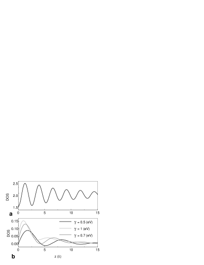
Figure 1: (a) DOS as a function of the distance $z$ from the boundary in FM in the zero approximation. (b) The additional term to the DOS as a function of the distance $z$ from the boundary in FM for $\omega=0$ and three different values of s-d electron scattering parameter $\gamma$ ($k_{Fs}^{\uparrow}=1.2$ $\AA^{-1}$, $k_{Fs}^{\downarrow}=0.42$ $\AA^{-1}$, $(\Delta\gamma)^{2}=0.1$ $eV^{2}$).

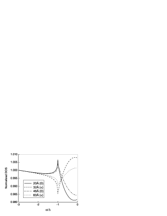
Figure 2: Energy variation of the DOS in FM for different distances $z$ from the boundary. Zero energy corresponds to the Fermi level, energy gap $\Delta=1.4$ meV, exchange field $h=10$ meV.

On the FM side, the proximity effect induces the superconducting order parameter. Increasing the distance from the interface it displays a damped oscillation and changes sign from positive to negative. Usually the states corresponding to a positive sign of superconducting order parameter are called the ”0 state” and those corresponding to a negative sign of order parameter the ”$\pi$ state”. In ref.Guoya2002 Guoya et al. develop a quantum-statistical approach based on the McMillan and BTK theories to calculate the DOS dependence on the energy. They show that the DOS in FM displays a maximum at the energy-gap edge and a minimum at the Fermi level exhibiting the SC-like shape for the ”0” state, and flipped shape for the ”$\pi$” state.

Figure 2 shows the result of our calculations of the DOS in FM using the Gor’kov equations. As it may be seen the DOS exhibits the same as in ref. Guoya2002 peak-dip behavior near the SC gap for ”0” and ”$\pi$” states. With increasing the distance from the interface, the SC-like behavior of the DOS in F-layer gradually disappears. Such two different DOS shapes in FM near the FM/SC boundary for the ”0” and ”$\pi$” states have been observed experimentally by Kontos et al. Kontos2000 in the measurements of the DOS by planar-tunnelling spectroscopy in $Al/Al_{2}O_{3}/PdNi/Nb$ junctions.

On the SC side the superconducting order parameter is diminished near the FM/SC interface (see Fig. 3) and owing to the proximity effect the superconductivity in the SC near the interface also becomes gapless. Far from the boundary the DOS in SC takes it usual shape as in bulk superconductor.

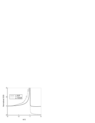
Figure 3: Energy variation of the DOS in the SC near (solid line) and far (dotted line) from the boundary.

This work was supported by the Russian Foundation for Basic Research (grant N 04-02-16688 a).

References

(1)
A. Buzdin, Phys.Rev. B 62 (2000) 11377.
(2)
R. Fazio, and C. Lucheroni, Europhysics Lett. 45 (1999) 707.
(3)
F. B. Bergeret, A. V. Volkov, and K. B. Efetov, Phys. Rev. B
65 (2002) 134505.
(4)
Guoya Sun, D. Y. Xing, J. Dong, M. Liu, Phys.Rev. B 65
(2002) 174508.
(5)
T. Kontos, M. Aprili, J. Lesueur, and X. Grison, Phys.Rev.Lett.
86 (2000) 304.