Long Chaotic Transients in Complex Networks

Abstract

We show that long chaotic transients dominate the dynamics of randomly diluted networks of pulse-coupled oscillators. This contrasts with the rapid convergence towards limit cycle attractors found in networks of globally coupled units. The lengths of the transients strongly depend on the network connectivity and varies by several orders of magnitude, with maximum transient lengths at intermediate connectivities. The dynamics of the transient exhibits a novel form of robust synchronization. An approximation to the largest Lyapunov exponent characterizing the chaotic nature of the transient dynamics is calculated analytically.

The dynamics of complex networks nw_struct is a challenging research topic in physics, technology and the life sciences. Paradigmatic models of units interacting on networks are pulse- and phase-coupled oscillators strog:01 . Often attractors of the network dynamics in such systems are states of collective synchrony ernst:95 ; gerst:96 ; mirollo:90 ; pesk:84 ; twg:02a ; twg:02b ; sync ; bressloff ; hansel ; herz . Motivated by synchronization phenomena observed in biological systems, such as the heart pesk:84 or the brain sing:89 , many studies have investigated how simple pulse-coupled model units can synchronize their activity. Here a key question is whether and how rapid synchronization can be achieved in large networks. It has been shown that fully connected networks as well as arbitrary networks of non-leaky integrators can synchronize very rapidly mirollo:90 ; gerst:96 . Biological networks however, are typically composed of dissipative elements and exhibit a complicated connectivity.

In this Letter, we investigate the influence of diluted network connectivity and dissipation on the collective dynamics of pulse-coupled oscillators. Intriguingly, we find that the dynamics is completely different from that of globally coupled networks or networks of non-leaky units, even for moderate dissipation and dilution: long chaotic transients dominate the network dynamics for a wide range of connectivities, rendering the attractors (simple limit cycles) irrelevant. Whereas the transient length is shortest for very high and very low connectivity, it becomes very large for networks of intermediate connectivity. The transient dynamics exhibits a robust form of synchrony that differs strongly from the synchronous dynamics on the limit cycle attractors. We quantify the chaotic nature of the transient dynamics by analytically calculating an approximation to the largest Lyapunov exponent on the transient.

We consider a system of $N$ oscillators mirollo:90 ; ernst:95 that interact on a directed graph by sending and receiving pulses. For concreteness we consider asymmetric random networks in which every oscillator $i$ is connected to an other oscillator $j\neq i$ by a directed link with probability $p$. A phase variable $\phi_{j}(t)\in[0,1]$ specifies the state of each oscillator $j$ at time $t$. In the absence of interactions the dynamics of an oscillator $j$ is given by

$$\textrm{d}\phi_{j}(t)/\textrm{d}t=1\,.$$ (1)

When an oscillator $j$ reaches the threshold, $\phi_{j}(t)=1$, its phase is reset to zero, $\phi_{j}(t^{+})=0$, and the oscillator emits a pulse that is sent to all oscillators $i$ possessing an in-link from $j$. After a delay time $\tau$ this pulse induces a phase jump in the receiving oscillator $i$ according to

$$\phi_{i}((t+\tau)^{+}):=\min\{U^{-1}(U(\phi_{i}(t+\tau))+\varepsilon_{ij}),1\}$$ (2)

which depends on its instantaneous phase $\phi_{i}(t+\tau)$, the excitatory coupling strength $\varepsilon_{ij}\geq 0$, and on whether the input is sub- or supra-threshold. The phase dependence is determined by a twice continuously differentiable function $U(\phi)$ that is assumed to be strictly increasing, $U^{\prime}(\phi)>0$, concave (down), $U^{\prime\prime}(\phi)<0$, and normalized such that $U(0)=0$ and $U(1)=1$ (cf. mirollo:90 ; TWG:03a ).

This model, originally introduced by Mirollo and Strogatz mirollo:90 , is equivalent to different well known models of interacting threshold elements if $U(\phi)$ is chosen appropriately (cf. TWG:03a ). The results presented in this Letter are obtained for $U_{b}(\phi)=b^{-1}\ln(1+(e^{b}-1)\phi)$, where $b>0$ parameterizes the curvature of $U$, that determines the strength of the dissipation of individual oscillators. The function $U$ approaches the linear, non-leaky case in the limit $\lim_{b\rightarrow 0}U_{b}(\phi)=\phi$. Other nonlinear choices of $U\neq U_{b}$ give results similar to those reported below. The considered graphs are strongly connected, i.e. there exists a directed path from any node to any other node. We normalize the total input to each node $\sum_{j=1}^{N}\varepsilon_{ij}=\varepsilon$ such that the fully synchronous state ($\phi_{i\ }(t)\equiv\phi_{0}(t)$ for all $i$) exists twg:02b . Furthermore for any node $i$ all its $k_{i}$ incoming links have the same strength $\varepsilon_{ij}=\varepsilon/k_{i}$ .

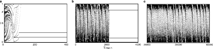
Figure 1: Long chaotic transients towards periodic attractor states in complex networks. The panels show the dynamics of random networks of $N=100$ oscillators ($b=1.0,$ $\varepsilon=0.1$, $\tau=0.1$). The phases of all oscillators are marked along the vertical axis just after an arbitrary but fixed reference oscillator is reset. Time is thus measured by the number of resets $n$ of the reference oscillator. The length of the transients increases quickly with dilution: (a) for the fully connected ($p=1$) network the transient length is $T\approx 10^{2}$, whereas (b) $T\approx 2\cdot 10^{3}$ for $p=0.97$ and (c) no attractor reached up to $n=10^{5}$ ($T>10^{5}$) for $p=0.80$.

Numerical investigations of all-to-all coupled networks ($p=1$) show rapid convergence from arbitrary initial conditions to periodic orbit attractors (cf. mirollo:90 ; twg:02a ), in which several synchronized groups of oscillators (clusters) coexist ernst:95 ; twg:02a . In general we find that the transient length $T$, i.e. the time the system needs to reach an attractor, is short for all-to-all coupled networks and depends only weakly on network size, for instance $T\approx 10^{2}$ for $N=100$ oscillators [see e.g. Fig. 1(a)].

In contrast to fully connected networks, diluted networks exhibit largely increased transient times: eliminating just $3\%$ of the links ($p=0.97$) leads to an increase in $T$ of one order of magnitude [$T\approx 10^{3}$, Fig. 1(b)]. The system finally settles on an attractor which is similar to the one found in the fully connected network, i.e. a periodic orbit with several synchronized clusters. Further dilution of the network causes the transient length to grow extremely large [$T>10^{5}$, Fig. 1(c)]. The lifetime of an individual transient typically depends strongly on the initial condition. We observed the dynamics started from many randomly chosen initial phase vectors distributed uniformly in $[0,1]^{N}$ and typically find a wide range of transient times (Fig. 2).

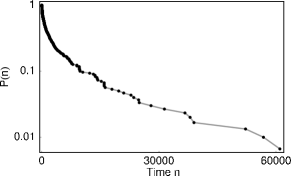
Figure 2: Typical transients in complex networks are very long. Distribution of transient lengths on randomly diluted networks ($N=16$, $p=0.8$, $b=3$, $\varepsilon=0.1,\,\tau=0.1$, histogram of 300 random networks).

Figure 3: The average transient length $\langle T\rangle$ depends non-monotonically on the network connectivity $p$. The longest transients are found for intermediate connectivities. Average over 100 initial conditions ($N=16$, $b=3,\varepsilon=0.1,\,\tau=0.1$). Error bars are standard error of mean. The inset shows the rapid growth of $\langle T\rangle$ with network size $N$ (boxes: $p=0.8$, stars: $p=0.95$, diamonds: $p=1.0$ ).

We systematically studied the average transient length in dependence on the average connectivity $p$. Surprisingly the average transient length, a dynamical feature of the network, depends non-monotonically on the network connectivity $p$ (Fig. 3 ), whereas many structural properties of random graphs such as the average path length between two vertices are monotonic in $p$ bolobas . The average transient length is short for low and high connectivity values $p$, but becomes very large for intermediate connectivities, even for only weakly diluted networks. Moreover we find that the mean lifetime $\langle T\rangle$ grows exponentially with the network size $N$ for diluted networks whereas it is almost independent of network size for fully-connected networks (inset of Fig. 3). This renders long transients the dominant form of dynamics for all but strongly diluted or fully connected networks. The transient length defines a new, collective time scale that is much larger than the natural period, $1$, of an individual oscillator and the delay time, $\tau$, of the interactions. This separation of time scales makes it possible to statistically characterize the dynamics on the transient (cf. ttel:91 ).

What are the main features of the transient dynamics? We determined the statistical distribution of phases of the oscillators during the transient. Interestingly the oscillators exhibit a novel kind of synchrony during the transient: most of the units form a single, roughly synchronized cluster (Fig. 4). This cluster is robust in the sense that it always contains approximately the same number of oscillators with the same spread of relative phases although it continuously absorbs and emits oscillators. On the attractor, however, the oscillators are organized in several precisely synchronized clusters (cf. Fig. 4), such that the transient dynamics is completely different from the dynamics on the attractor.

Numerically we find that nearby trajectories diverge exponentially with time, an indication of chaos [Fig. 5(a)]. To further quantify the chaotic nature of the transient dynamics, we determined the speed of divergence of two nearby trajectories both by numerical measurements and by analytically estimating the largest Lyapunov exponent on the transient. Let {$t_{n}$: $n\in\mathbb{N}_{0}$} be a set of firing times of an arbitrary, fixed reference oscillator and $\phi_{i}^{1}(t_{n}),\phi_{i}^{2}(t_{n})$, $i\in\{1,\dots,N\}$, the set of phases of all oscillators $i$ of two transient trajectories 1 and 2. We then define the distance

$$D_{n}:=\sum_{i=1}^{N}|\phi_{i}^{1}(t_{n})-\phi_{i}^{2}(t_{n})|_{c}$$ (3)

between these two trajectories at time $t_{n}$ where $|\cdot|_{c}$ denotes the distance of two points on a circle with circumference 1. For a small initial separation $D_{0}\ll 1$ at time $t_{0}$ the distance $D_{n}$ at later time $t_{n}$ scales like [Fig. 5(a)]

$$D_{n}\approx D_{0}e^{\Lambda n}\,,$$ (4)

quantifying the speed of divergence by the largest Lyapunov exponent $\Lambda$. To analytically estimate $\Lambda$, we determine the phase advance of oscillator $i$ evoked by a single pulse received from oscillator $j$,

$$\phi_{i}(t^{+})=a_{ij}\phi_{i}(t)+c_{ij}\,,$$ (5)

where we have used the definition of $U_{b}(\phi)$ in Eq. (2) and considered only sub-threshold input. We obtain

$$a_{ij}:=\exp(b\varepsilon_{ij})\geq 1\,,$$ (6)

independent of the delay $\tau$ and the constants $c_{ij}$ which are independent of $\phi_{j}(t)$. The magnitude by which a single pulse increases the difference $|\phi_{i}^{1}(t^{+})-\phi_{i}^{2}(t^{+})|_{c}=a_{ij}|\phi_{i}^{1}(t)-\phi_{i}^{2}(t)|_{c}$ is thus only determined by $a_{ij}$. If an oscillator $i$ receives exactly one pulse from all its upstream (i.e. presynaptic) oscillators between $t_{n}$ and $t_{n+1}$, the total increase due to all these pulses is determined by

$$A_{i}:=\prod_{j=1}^{N}a_{ij}=\exp\left(b\sum_{j=1}^{N}\varepsilon_{ij}\right).$$ (7)

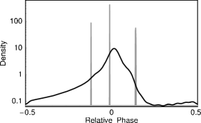
Figure 4: The oscillators form a single, slightly dispersed cluster during the transient (black) and several precisely synchronized clusters on the attractor (grey). The figure shows the density of phases of the oscillators relative to their average phase. Data shown for the dynamics displayed in Fig. 1(b) averaged over $n=500\dots 1500$ (transient) and $n=2500\dots 3500$ (attractor).

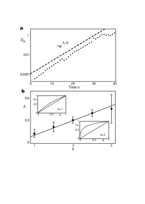
Figure 5: (a) The distance $D_{n}$ between two nearby trajectories grows exponentially with time $n$. The slope of the dashed line quantifies the rate of divergence measured by the largest Lyapunov exponent $\Lambda$. The jumps at $n=16$ and $n=29$ are due to the choice of the reference oscillator. (b) The largest Lyapunov exponent $\Lambda$ depends linearly on the curvature $b$ of the interaction function $U_{b}$. These numerical results (disks with error bars) agree with the analytical prediction $\Lambda=b\cdot\varepsilon$ (continuous line) bdeviation . Error bars denote the standard deviation for 100 random networks ($N=100$, $p=0.75$, $\varepsilon=0.1,\,\tau=0.1$). Inset: interaction function $U_{b}(\phi)$ for $b=1$ and $b=5$.

The normalization $\sum_{j=1}^{N}\varepsilon_{ij}=\varepsilon$ implies $A_{i}=\exp(b\varepsilon)=:A$ for all oscillators $i$. Noting that the network is in an asynchronous state during the transient and assuming that between $t_{n}$ and $t_{n+1}$ each oscillator fires exactly once we find $D_{n+1}\approx AD_{n}$. The largest Lyapunov is then approximated by

$$\Lambda\approx\ln A=b\cdot\varepsilon.$$ (8)

Numerical results are in good agreement with Eq. (8) for intermediate values of $b$ [bdeviation , see Fig. 5(b)]. Note that there is no free parameter in Eq. (8). This calculation shows that the curvature $b$ of $U_{b}$ and the coupling strength $\varepsilon$ strongly influence the dynamics during the transient by determining the largest Lyapunov exponent. To further characterize the dynamics we investigated return maps of inter spike intervals (i.e. the time between two consecutive resets of individual oscillators). This analysis revealed broken tori in phase space (not shown). Moreover we find that the correlation dimension grassberger of the transient orbit is low (e.g. $D_{\text{{corr.}}}\approx 5$ for $N=100,$ $p=0.96$ and $b=3,\,\varepsilon=0.1,\,\tau=0.1$). This indicates that the chaotic motion during the transient takes place in the vicinity of quasiperiodic motion on a low dimensional toroidal manyfold in phase space. Interestingly quasiperiodic motion was also found in fully-connected networks of similar integrate-and-fire oscillators vrees:96a .

How do the long chaotic transients come into existence? As a first step towards answering this question we investigated in which region of parameter space long chaotic transients occur. It turned out that they do not sensitively depend on parameters but prevail for a substantial region of parameter space in randomly diluted networks. The region covered by long transients in parameter space (not shown) is similar to that covered by unstable attractors for fully connected networks (cf. twg:02a ). As, in general, long chaotic transients often occur in situations like crises or attractor destructions tel:94 , we conjecture that long transients occur in this system because diluting the network converts unstable attractors that prevail in phase space into unstable (presumably non-attracting) periodic orbits, inducing sensitive dependence on initial conditions and thus chaotic transient dynamics. The interesting open question about the dynamical origin of the transient needs further investigation.

In summary, we described a novel type of dynamics in complex networks of pulse-coupled oscillators: long chaotic transients. These transients dominate the dynamics for a wide range of parameters and become prevalent for large networks, thus rendering the dynamics on the attractors irrelevant to the observed behavior. This is in stark contrast to the rapid convergence found in fully connected networks as well as in networks of non-leaky elements. The transient length defines a new, collective timescale that is not present in the single unit dynamics. Interestingly it is maximal for intermediate connectivities in contrast to many structural network properties. The transient dynamics exhibits a rapid and robust form of synchronization: the oscillators form a roughly synchronized cluster. For the transient dynamics we approximately calculated the largest Lyapunov exponent analytically; this is rarely possible for any high dimensional system. The approximation is in good quantitative agreement with the exponential divergence of nearby trajectories found in numerical simulations.

Previous studies on the synchronization dynamics of pulse-coupled oscillators have focused on globally coupled networks or on systems of individual elements without dissipation (see e.g. ernst:95 ; gerst:96 ). Our results show that the combination of dissipation and complex connectivity can create a qualitatively distinct network dynamics. More generally, our results emphasize that the network’s structure can have a major impact on its dynamics, as small structural changes induce fundamentally different forms of behavior. This is very likely to occur not only in networks of coupled oscillators but in many other complex networks, too.

This research was supported in part by the National Science Foundation under Grant No. PHY99-07949.

References

- (1) S. Bornholdt and H.G. Schuster (Eds.), Handbook of Graphs and Networks, (Wiley-VCH, Weinheim, 2002); R. Albert and A.-L. Barabási, Rev. Mod. Phys. 74, 47 (2002); S. N. Dorogovtsev and J. F. F. Mendes, Adv. Phys. 51, 1079 (2001).
- (2) S.H. Strogatz, Nature 410, 268 (2001).
- (3) C. Peskin, Mathematical Aspects of Heart Physiology, (Courant Institute of Mathematical Sciences, New York University, 1975).
- (4) A.T. Winfree, The Geometry of Biological Time (Springer, New York, 2001); L. Glass, Nature 410, 277 (2001).
- (5) R.E. Mirollo and S.H. Strogatz, SIAM J. Appl. Math. 50, 1645 (1990).
- (6) U. Ernst, K. Pawelzik, and T. Geisel, Phys. Rev. Lett. 74, 1570 (1995).
- (7) A. V. M. Herz, J. J. Hopfield, Phys. Rev. Lett. 75, 1222 (1995).
- (8) W. Gerstner, Phys. Rev. Lett. 76, 1755 (1996).
- (9) P. C. Bressloff and S. Coombes, Phys. Rev. Lett. 81, 2384 (1998).
- (10) D. Hansel and G. Mato, Phys. Rev. Lett. 86, 4175 (2001).
- (11) M. Timme, F. Wolf and T. Geisel, Phys. Rev. Lett. 89, 154105 (2002).
- (12) M. Timme, F. Wolf and T. Geisel, Phys. Rev. Lett. 89, 258701 (2002).
- (13) C.M. Gray, P. König, A.K. Engel, and W. Singer, Nature 338, 334 (1989).
- (14) M. Timme, F. Wolf, and T. Geisel, Chaos 13, 377 (2003).
- (15) B. Bollobás, Random Graphs, Second Edition, (Cambridge University Press, 2001).
- (16) T. Tél, Transient Chaos in Directions in Chaos (H. Bai-Lin (ed.), World Scientific, Singapore, 1990); T. Tél, J. Phys. A: Math. Gen. 24, L1359 (1991).
- (17) For values of outside of the range shown in Fig. 5 deviations exist because not all oscillators fire exactly once during one cycle. For small we observe irregular dynamics that is markedly different from that shown in Fig. 1; we find in particular that individual oscillators remain in the dynamic cluster for a long time which compromises the approximation of an asynchronous state during the transient. For large the bent character of gets more and more kink-like. Thus more pulses are supra-threshold, the dynamics is strongly influenced by phase resets and thus not adequately described by Eq. (5).
- (18) P. Grassberger and I. Procaccia, Physica D 9, 189 (1983).
- (19) C. van Vreeswijk, Phys. Rev. E. 54, 5522 (1996).
- (20) I.M. Jánosi, L. Flepp, and T. Tél, Phys. Rev. Lett. 73, 529 (1994).