Effects of large disorder on the Hofstadter butterfly

Abstract

Motivated by the recent experiments on periodically modulated, two dimensional electron systems placed in large transversal magnetic fields, we investigate the interplay between the effects of disorder and periodic potentials in the integer quantum Hall regime. In particular, we study the case where disorder is larger than the periodic modulation, but both are small enough that Landau level mixing is negligible. In this limit, the self-consistent Born approximation is inadequate. We carry extensive numerical calculations to understand the relevant physics in the lowest Landau level, such as the spectrum and nature (localized or extended) of the wave functions. Based on our results, we propose a qualitative explanation of the new features uncovered recently in transport measurements.

I Introduction

Two-dimensional electron systems (2DES) placed in a uniform perpendicular magnetic field exhibit a rich variety of phenomena, such as the integerIQHE and fractionalFQHE quantum Hall effects. Springer Another well-studied problem is that of a 2DES in a uniform perpendicular magnetic field subjected to a periodic potential. Even before the discovery of the quantum Hall effects, HofstadterHofst showed that in this case, the electronic bands split into a remarkable fractal structure of subbands and gaps, the so-called Hofstadter butterfly. Two “asymptotic” regimes are usually considered: (i) if the magnitude of the periodic potential is very large compared to the cyclotron energy and the Zeeman splitting, then one can use lattice models to describe the hopping of electrons between Wannier-like states localized at the minima of the periodic potential, whereas (ii) if the magnitude of the periodic potential is small compared to the cyclotron energy, the periodic potential lifts the degeneracy of each Landau level. In both cases, the resulting butterfly structure is a function only of the ratio between the flux $\phi=B{\cal A}$ of the magnetic field through the unit cell of the periodic lattice, and the elementary magnetic flux $\phi_{0}=hc/e$. Remarkably, if $\phi/\phi_{0}$ of the first asymptotic case is equal to $\phi_{0}/\phi$ of the second case, their electronic structures are solutions of the same Harper’s equation.equiv If the periodic potential is comparable to the cyclotron energy, Landau level mixing must be taken into account; although Landau levels still split into subbands, the structure is no longer universal, but depends also on the ratio of the periodic potential amplitude and the cyclotron energy.germans

Experimentally, the case with a small periodic modulation can be realized more easily. This is because the periodic potential is usually imprinted at some distance from the 2DES layer; as a result, its magnitude in the 2DES is considerably attenuated. The interesting cases to study experimentally also correspond to small values of $\phi/\phi_{0}$ (of order unity), where the butterfly structure shows a small number of subbands separated by large gaps, and should therefore be easier to identify. Periodic modulations have been created using lithographyHolland ; Weimann ; Weiss and holographic illumination. Wulf The lattice constants of the resulting square lattices are of order 100 nm. As a result, the condition $\phi/\phi_{0}\approx 2$ (for instance) is satisfied for $B\approx 0.8$ T. This is a very low value, in the Shubnikov-de Haas (SdH) regime, not the high-$B$ quantum regime. Significant Landau level mixing and complications from the fact that the Fermi level is inside one of the higher Landau levels for such small $B$-values make the identification of the Hofstadter structure difficult.

Recently, a new method for lateral periodic modulation has been developed using a self-organized ordered phase of a diblock copolymer deposited on a GaAs/AlGaAs heterostructure.Sorin The polymer spheres create a 2D triangular lattice with a lattice constant of about 39 nm. The corresponding unit cell area is almost an order of magnitude smaller than those achieved in previous experiments, implying that the condition $\phi/\phi_{0}\approx 2$ is now satisfied for very strong magnetic fields, $B\approx 6$ T. At such high magnetic fields the system is in the strong quantum regime, and Landau level mixing can be safely ignored. For the experimental 2DES electron concentrations, the Fermi level is in the spin-down lowest Landau level.Sorin As a result, this experimental setup appears more promising for the successful observation of the butterfly.

Nevertheless, one must take into account the disorder which is present in the system (without disorder, there is no integer Quantum Hall Effect – IQHE – to begin with). If the disorder is very small compared to the periodic potential amplitude, one expects that the subbands of the Hofstadter structure are “smeared” on a scale $\hbar/\tau$, where $\tau$ is the scattering time, and $\tau\rightarrow\infty$ as disorder becomes vanishingly small. As a result, the larger gaps in the Hofstadter structure should remain open at the positions predicted in the absence of disorder, and one expects a series of minima in the longitudinal conductivity as the Fermi level traverses such gaps. The experiment indeed shows a very non-trivial modification of the longitudinal resistivity, with many peaks and valleys appearing in what is (in the absence of the periodic modulation) a smooth Lorentz-like peak.Sorin However, the position of the minima in $\rho_{xx}$ do not track the positions of the main gaps in the corresponding Hofstadter butterfly structure. Instead, the data suggests that in this experimental setup, disorder is not small, but rather large compared to the estimated amplitude of the periodic potential. This is not a consequence of poor samples, since these 2DES have high mobilities. It is due to the fact that the periodic modulation is considerably attenuated in the 2DES, leading to a small energy scale for the Hofstadter butterfly spectrum as compared to $\hbar/\tau$. As a result, the Hofstadter structure predicted in the absence of disorder is of little use for interpreting the experimental data. One might expect that in this case the periodic potential should have basically no effect on the disorder-broadened Landau level. This is indeed true for the strongly localized states at the top and bottom of the Landau level. However, states in the center of the Landau level extend over many unit cells of the periodic potential, and, as we demonstrate in the following, are non-trivially modified by its presence.

In this paper, we investigate numerically the behavior of a 2DES subject to a perpendicular magnetic field, a periodic potential and a disorder potential, under conditions applicable to the experimental system. The effective electron mass in GaAs is $0.067m_{e}$ while the magnetic fields of interest are on the order of 10 T. Under these conditions, the cyclotron energy $\hbar\omega_{c}$, of the order of 200 K, is the largest energy scale in the problem. The Zeeman energy $g^{*}\mu_{B}B$ for these fields is roughly 3 K, but electron interaction effects lead to a considerable enhancement of the spin splitting between the (spin polarized) Landau levels, which has been measured to be 20 K.Sorin2 The amplitude of the periodic potential’s largest Fourier components is estimated to be of the order of 1 K, and the scattering rate from the known zero field mobility is estimated to be $\hbar/\tau\sim 8$ K. Chaikin As a result of this ordering of energy scales, we neglect Landau level inter-mixing and study non-perturbatively the combined effects of a periodic and a large smooth disorder potential on the electronic structure of the lowest Landau level. Previously, the effects of small disorder on a Hofstadter butterfly have been perturbatively investigated using the self-consistent Born approximation (SCBA), MacDonald and the combined effect of white-noise disorder and periodic modulation on Hall resistance was studied following the scaling theory of IQHE.Huckestein Our results reveal details of the electronic structure not investigated previously.

The two-lead geometry we consider is schematically shown in Fig. 1: the finite 2DES is assumed to have periodic boundary conditions in the $y$-direction (along which the Hall currents flow), and is connected to metallic leads at the $x=-L_{x}/2$ and $x=+L_{x}/2$ edges. In particular, in this paper we study the effects of the periodic potential on the extended states carrying longitudinal currents between the two leads, and identify a number of interesting properties, in qualitative agreement with simple arguments provided by a semi-classical picture. Our main conclusion is that while the beautiful Hofstadter structure is destroyed by large disorder, the system still exhibits very interesting and non-trivial physics.

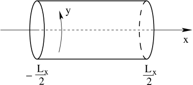
Figure 1: The two-lead geometry considered: the finite-size 2DES has periodic boundary conditions in the $y$-direction, and is attached to metallic leads at the $x=\pm L_{x}/2$ ends.

The paper is organized as follows: in Section II we briefly review the computation of the Hofstadter structure for a small-amplitude periodic potential. In Section III we describe the type of disorder potentials considered. Section IV describes the numerical methods used to analyze the spectrum and the nature of the electronic states, with both semi-classical and fully quantum-mechanical formalisms. Results are presented in Section V, while Section VI contains discussions and a summary of our conclusions.

II Periodic Potential

To clarify our notation, we briefly review the problem of a free electron of charge $-e$ moving in a 2D plane (from now on, the $xy$-plane, of dimension $L_{x}\times L_{y}$) in a magnetic field ${\bf B}=B{\bf e}_{z}$ perpendicular to the plane, as described by

$${\cal H}={1\over 2m}\left({\bf p}+{e\over c}{\bf A}\right)^{2}-{1\over 2}g\mu_{B}\vec{\sigma}\cdot{\bf B}$$

In the Landau gauge ${\bf A}=(0,Bx,0)$, the eigenfunctions of the Schrödinger equation ${\cal H}|n,k_{y},\sigma\rangle=E_{n,\sigma}|n,k_{y},\sigma\rangle$ are:

$$\langle{\bf r}|n,k_{y},\sigma\rangle={e^{-ik_{y}y}\over\sqrt{L_{y}}}e^{-{1\over 2}\left({x\over l}-lk_{y}\right)^{2}}{H_{n}\left({x\over l}-lk_{y}\right)\over\sqrt{2^{n}n!\sqrt{\pi}l}}\chi_{\sigma},$$ (1)

with eigenenergies

$$E_{n,\sigma}=\hbar\omega_{c}\left(n+{1\over 2}\right)-{1\over 2}g\mu_{B}B\sigma.$$ (2)

Here $l=\sqrt{\hbar c/eB}$ is the magnetic length, $\omega_{c}={eB/mc}$ is the cyclotron frequency, $H_{n}(x)$ are the Hermite polynomials and $\chi_{+1}^{T}=(1\;0)$, respectively $\chi_{-1}^{T}=(0\;1)$ are the eigenspinors of $\sigma_{z}$: $\sigma_{z}\chi_{\sigma}=\sigma\chi_{\sigma}$.

The degeneracy of a Landau level is given by the number of distinct $k_{y}$ values allowed. Imposing cyclic boundary conditions in the $y$-direction, we find

$$k_{y}={2\pi\over L_{y}}j,$$ (3)

where $j$ is an integer. The allowed values for $j$ are found from the condition that the electron wave-functions, which are centered at positions $x_{j}=l^{2}k_{y}=l^{2}2\pi j/L_{y}$ [see Eq. (1)] are within the boundary along the $x$-axis, i. e. $-L_{x}/2<x_{j}\leq L_{x}/2$. It follows that the degeneracy of each Landau level is $N=L_{x}L_{y}B/\phi_{0}$, with $\phi_{0}=hc/e$.

Consider now the addition of a periodic potential, with a lattice defined by two non-collinear vectors ${\bf a}_{1}$ and ${\bf a}_{2}$, such that $V({\bf r})=V({\bf r}+n{\bf a}_{1}+m{\bf a}_{2})$ for any $n,m\in{\cal Z}$. The periodic potential has non-vanishing Fourier components only at the reciprocal lattice vectors ${\bf g}=h{\bf g}_{1}+k{\bf g}_{2}$, where ${\bf g}_{i}\cdot{\bf a}_{j}=2\pi\delta_{ij}$ and $h,k$ are integers. Thus:

$$V({\bf r})=\sum_{{\bf g}}V_{{\bf g}}e^{i{\bf r\cdot g}}.$$ (4)

Further, since $V({\bf r})$ is real, it follows that $V_{{\bf g}}=V^{*}_{-{\bf g}}$.

In the absence of Landau level mixing, the Hofstadter spectrum for both squareHofst

$$V_{s}(x,y)=2A\left[\cos{2\pi\over a}x+\cos{2\pi\over a}y\right],$$ (5)

and triangularWannier

$$V_{t}(x,y)=-2A\left[\cos{4\pi\over\sqrt{3}a}x+\cos{2\pi\over\sqrt{3}a}\left(x-y\sqrt{3}\right)\right.$$

$$\left.+\cos{2\pi\over\sqrt{3}a}\left(x+y\sqrt{3}\right)\right]$$ (6)

periodic potentials, with nonzero Fourier components only for the shortest reciprocal lattice vectors, have been studied extensively in the literature.Hofst ; Wannier ; Geisel ; Gerhardts The parameter defining the spectrum is the ratio between the flux $\phi={{\bf B}}\cdot({\bf a}_{1}\times{\bf a}_{2})$ of the magnetic field through a unit cell and the elementary flux $\phi_{0}$. For $\phi/\phi_{0}=q/p$, where $p$ and $q$ are mutually prime integers, the original Landau level is split into $q$ sub-bands.

We would like to emphasize a qualitative difference between the two types of potentials: the square potential in Eq. (5) is particle-hole symmetric, since $V_{s}(x,y)=-V_{s}(x+{a\over 2},y+{a\over 2})$. As a result, the sign of its amplitude is irrelevant. On the other hand, the triangular potential does not have this symmetry. With the sign chosen in Eq. (6) and $A>0$, $V_{t}$ has deep local minima at the sites of the triangular lattice, whereas the maxima are relatively flat and located on a (displaced) honeycomb lattice. As a result, the sign of $V_{t}$ is highly relevant. The second fact that must be mentioned is that the choice made in Eqs. (5) and (6) is rather simple, since it aligns the periodic potential with the edges of the sample in a very specific way. In general, however, one could consider the case where the periodic lattice is rotated by some finite angle with respect to the sample edges; study of such cases will be discussed in future work. Finally, it may seem that this choice of periodic potentials is very restrictive also because only the shortest lattice vectors have been kept in the Fourier expansion. In fact, the methods we employ can be directly used for potentials with more Fourier components, but their inclusion leads to no new physics.

III Disorder Potential

Real samples always have disorder. The current consensus is that high-quality GaAs/AlGaAs samples exhibit a slowly varying, smooth disorder potential. In a semi-classical picture, the allowed electron trajectories in the presence of such disorder follow its equipotential lines.Springer ; Trugman Closed trajectories imply localized electron states, while extended trajectories connecting opposite edges of the sample are essential for current transport through the sample (for more details, see Sec. IV.1).

In typical experimental setups,Sorin dopant Si impurities with a concentration of $\sim 10^{13}$ cm^-2 are introduced in a thin layer of 6 nm in thickness, located 20 nm above the GaAs/AlGaAs interface. Typically, up to 10% of the Si atoms are ionized. A small fraction of the ionized electrons migrate to the GaAs/AlGaAs interface where they form the 2D electron gas. The electrostatic potential created by the ionized impurities left behind is the major source of disorder in the 2DES layer. On the length-scale we are interested in, there are $10^{4}$ to $10^{5}$ such ionized Si impurities per $\mu m^{2}$. The resulting disorder potential must be viewed as a collective effect of the density fluctuation of the ionized impuritiesNixon rather than a simple summation of the Coulomb potential of a few impurities. The electrostatic potential from Si impurities is compensated and partially screened by other mobile negative charges in the system such as, for example, the surface screening effect by mirror charges considered by Nixon and Davies.Nixon An exact treatment of this problem is difficult, since one should consider the spatial correlation of the ionized impurities. Stopa ; DasSarma One model used to describe such disorder consists of randomly placed Gaussian scatterers.Ando This model captures the main feature of a smooth disorder potential and supports classical trajectories on equipotential contours, but it has no natural energy/length scales associated with it. As a result, here we choose to also investigate a different model of the disorder, which incorporates the smooth character of the Coulomb potential in real space.

We generate a realization of the disorder potential in the following way: positive and negative charges, corresponding to a total concentration of $10^{3}\,\mu m^{-3}$ are randomly distributed within a volume $[-L_{x}/2,L_{x}/2]\times[-L_{y}/2,L_{y}/2]\times[20\mbox{nm}+d,26\mbox{nm}+d]$ above the electron gas which is located in the $z=0$ plane. Here, we choose $d=4$ nm as an extra spacer since the electronic wave-functions are centered about 3-5 nm below the GaAs/AlGaAs interface. Since we are not simulating single impurities but density fluctuations, these charges are not required to be elementary charges. Instead, we use a uniform distribution in the range $[-e,e]$ for convenience (a Gaussian distribution would also be a valid choice), and sum up all Coulomb potentials from these charges, using the static dielectric constant in GaAs $\epsilon=12.91$.Ralph The resulting disorder potential has energy and length scales characteristic of the real samples. Typical contours for such potentials are shown in Sec. V.

In an infinite system, in the quantum Hall regime, the existence of quantum Hall steps implies the existence of critical energies at which the localization length diverges.Halperin This is the quantum analog of the two dimensional percolation problem in a smooth random landscape, for which there exists a single critical energy.Trugman In the case of potentials with electron-hole symmetry $\left<V({{\bf r}})\right>=0$, the critical energy lies in the middle of the band ($E_{c}=0$), leading to percolating path at half filling. For a finite mesoscopic sample, however, not only does the percolating path (critical energy) $E_{c}$ deviate from this value, but in samples without a periodic boundary condition one need not have a percolating path traversing the system in the desired direction. This arises from the fluctuations near the edge of a mesoscopic system with free boundary conditions.

We circumvent such a possibility by adding an extra smooth potential $V^{\prime}(x,y)$ to the impurity-induced disorder potential $V_{i}(x,y)$, such that the total potential $V=V_{i}+V^{\prime}$ is zero on the opposite edges $x=\pm L_{x}/2$ of the sample where the metallic leads are attached. The supplementary contribution $V^{\prime}(x,y)$ can be thought of as simulating the effect of the leads on the disorder potential, since the metallic leads hold the potential on each edge constant by accumulating extra charges near the interface. Therefore, physically we expect that the extra potential $V^{\prime}$ decays exponentially over the screening length $\lambda$ inside the sample. This implies:

$$V^{\prime}(x,y)=-{V_{i}\left(-{L_{x}/2},y\right)+V_{i}(L_{x}/2,y)\over 2}{\cosh(x/\lambda)\over\cosh(L_{x}/2\lambda)}$$

$$+{V_{i}(-L_{x}/2,y)-V_{i}(L_{x}/2,y)\over 2}{\sinh(x/\lambda)\over\sinh(L_{x}/2\lambda)}$$

where $\lambda$ is taken to be $100$ nm in our calculation.

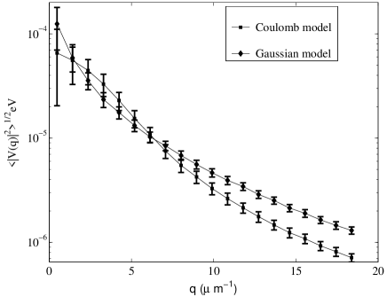
Figure 2: Averaged Fourier amplitudes of two types of disorder potential as a function of wavevector $q=|{{\bf q}}|$. For both Coulomb and Gaussian model, $V(q)^{2}$ is averaged over 116 disorder realizations. The relation between $V(q)$ and $V({\bf r})$ and relevant parameters are discussed in the text. The standard deviation, $(L_{x}L_{y})^{-1}\left<\int d{\bf r}V^{2}({\bf r})\right>$ for the Coulomb model is $3.2\times 10^{-7}$eV², and $2.1\times 10^{-7}$eV² for the Gaussian model.

In Fig. 2, we plot the average of Fourier transform of the magnitude of the random potential $\sqrt{\left<|V(q)|^{2}\right>}$ versus $q=|{{\bf q}}|$ for the Coulomb model and the Gaussian model. The Gaussian model is generated by adding 100 randomly placed Gaussian scatterers on an area of $3\mu m\times 3\mu m$, each contributing $A_{d}e^{-r^{2}/d^{2}}$, where $A_{d}$ is uniformly distributed in $[-2,2]$ meV, and $d$ is uniformly distributed in $[0,0.2]$ $\mu$m. $V({\bf q})$ is related to $V({\bf r})$ by $V({\bf r})=\sum_{{\bf q}}V({\bf q})e^{i{{\bf q}\cdot r}}$, where the summation is over all the wavevectors involved in the fast Fourier transformation. The Gaussian model has an arbitrary energy scale which is fixed by the maximum value of the distribution $A_{m}$. Here $A_{m}=2$ meV. As can be seen, $V(q)$ of both models are decreasing functions of $q$. The trends of decay are exponential at large $q$. At small $q$, the two models behave differently. Despite the difference, both models lead to the same qualitative results, although, as expected, minor quantitative differences are present. This shows that the physics we uncover is independent of the particular type of slowly-varying disorder potential considered, and therefore should be relevant for the real samples.

IV Numerical Calculations

In this section we discuss the numerical methods we use, including derivations of some relevant formulas. As already stated, we focus on the case where the amplitudes of the periodic and disorder potentials are very small compared to the cyclotron energy and the Zeeman splitting, and therefore inter-level mixing is ignored.

IV.1 Semi-classical treatment

The semi-classical approach is validTrugman for the integer quantum Hall effect in the presence of a slowly varying, smooth disorder potential and large magnetic fields (such as we consider), so that the magnetic length $l$ which determines the spatial extent of the electron wave-functions is much smaller than the length scale of variation of the smooth disorder potential, $|\nabla V({\bf r})|\ll\hbar\omega_{c}/l$. Then, semi-classically the electron moves along the equipotential contours of the disorder potential $V({\bf r})$, in the direction parallel to $\nabla V({\bf r})\times{\bf B}$. Since the kinetic energy is quenched in the lowest Landau level, the total energy of the electron simply equals the value of the disorder potential on the equipotential line on which its trajectory is located. As a result, the density of states in the semi-classical approach is directly given by the probability distribution for the disorder potential, which can be calculated by randomly sampling the potential energy and plotting a histogram of the obtained values.Trugman ; note1

In Sec. V we compare the results obtained within this semi-classical approach with fully quantum mechanical results. As expected, the agreement is good if only the disorder potential is present. However, if the periodic modulation is also included, the lattice constant $a$ provides a new length-scale which is comparable to the magnetic length $l$, and the semi-classical picture breaks down. Quantum mechanical calculations are absolutely necessary to quantitatively treat this case.

IV.2 Quantum Mechanical Treatment

As shown in Sec. II, for a finite sample of size $L_{x}\times L_{y}$ at a given magnetic field $B$, the degeneracy of the unperturbed Landau level is $N=L_{x}L_{y}B/\phi_{0}=L_{x}L_{y}/(2\pi l^{2})$. Since the disorder varies very slowly, we need to consider systems with $L_{x},L_{y}\gg l$ to properly account for its effects. As a result, the number of states in a Landau level can be as large as $10^{4}$ in our calculations. Storage of the Hamiltonian as a dense matrix requires considerable amount of computer memory and its direct diagonalization is prohibitively time-consuming. Sparse matrix diagonalization techniques could be employed, but they are less efficient when all eigenvectors are needed, and also have some stability issues.

Here we introduce the numerical methods we use to compute densities of states and infer the nature (localized or extended) as well as the spatial distribution of the wave-functions, while avoiding direct diagonalization.

IV.2.1 Matrix elements

Since inter-level mixing is ignored, the Hilbert subspaces corresponding to different spin-polarized Landau levels do not hybridize. Each Hilbert subspace $(n,\sigma)$ has a basis described by Eq. (1), containing $N$ orthonormal vectors indexed by different $k_{y}$ values.

In order to compute matrix elements of the total Hamiltonian in such a basis, we use the following identity derived in Ref. Gerhardts, (notice their different sign convention for $k_{y}$. If $\sigma\neq\sigma^{\prime}$, the overlap is zero):

$$\left<n^{\prime},k^{\prime}_{y}\right|e^{i{\bf q\cdot r}}\left|n,k_{y}\right>=\delta_{k^{\prime}_{y},k_{y}-q_{y}}{\cal L}_{n^{\prime},n}({\bf q})e^{{il^{2}\over 2}q_{x}(k^{\prime}_{y}+k_{y})},$$ (7)

where

$${\cal L}_{n^{\prime},n}({\bf q})=\left(m!\over M!\right)^{1\over 2}i^{|n^{\prime}-n|}\left[q_{x}+iq_{y}\over\sqrt{q_{x}^{2}+q_{y}^{2}}\right]^{n-n^{\prime}}$$

$$\times e^{-{1\over 2}Q}Q^{{1\over 2}|n^{\prime}-n|}L_{m}^{(|n^{\prime}-n|)}(Q),$$

with $Q={1\over 2}l^{2}(q_{x}^{2}+q_{y}^{2})$, $m$ and $M$ the minimum and the maximum of $n^{\prime}$ and $n$ respectively, and $L^{(|n^{\prime}-n|)}_{m}(Q)$ the associated Laguerre polynomial. When band-mixing is neglected $n=n^{\prime}$ and ${\cal L}_{n,n}({\bf q})=e^{-{1\over 2}Q}L_{n}(Q)$. For the first Landau level, $L_{0}(x)=1$.

Eq. (7) gives us the matrix elements for the square [Eq. (5)] or triangular [Eq. (6)] periodic potentials. In either case, there are Fourier components corresponding to $q_{y}=\pm 2\pi/a$ and $q_{y}=0$. Since only basis vectors for which the difference $k_{y}-k_{y}^{\prime}=q_{y}$ give non-vanishing matrix elements, we must choose the length $L_{y}$ of the sample to be a multiple integer of $a$, the lattice constant.

The matrix elements of the disorder potential are computed in a similar way. We use a grid of dimension $N_{x}\times N_{y}$ to cover the sample and generate the values of the disorder potential on this grid. Then, fast Fourier transform (FFT)FFT is used to find the long wavelength components of the disorder potential corresponding to the allowed values $q_{x,y}=0,\pm{2\pi\over L_{x,y}},...,\pm\left[{N_{x,y}\over 2}\right]{2\pi\over L_{x,y}}$ (proper care is taken to define Fourier components so that $V_{{\bf q}}=V^{*}_{-{\bf q}}$). The matrix elements of this discretized disorder potential are then computed using Eq. (7). In principle, finer grids (increased values for $N_{x}$ and $N_{y}$) will improve accuracy. However, they also result in longer computation times, since they add extra matrix elements in the sparse matrix, corresponding to large wave-vectors. We have verified that a grid size of dimension $N_{x}=N_{y}=72$ is already large enough to accurately capture the landscape of a $3\mu m\times 3\mu m$ sample and the computed quantities have already converged, with larger grids leading to hardly noticeable changes. This procedure is also justified on a physical basis. First, the neglected large wave-vector components describe very short-range spatial features, which are probably not very accurately captured by our disorder models to begin with, and which are certainly not believed to influence the basic physics. Secondly, this procedure insures that the actual disorder potential we use is periodic in the $y$-direction, since each Fourier component retained has this property. This is consistent with our use of a basis of wave-functions which are periodic along $y$.

The matrix elements of the Hamiltonian within a given Landau level $(n,\sigma)$ are then $\langle n,k_{y},\sigma|{\cal H}|n,k^{\prime}_{y},\sigma\rangle=E_{n,\sigma}+\langle n,k_{y}|{\cal V}|n,k^{\prime}_{y}\rangle$, where $E_{n,\sigma}$ are given by Eq. (2) and the matrix elements of both the periodic and the disorder part of the potential ${\cal V}$ are computed as already discussed. This produces a sparse matrix, which is stored efficiently in a column compressed format.

IV.2.2 Densities of States and Filling Factors

A quantity that can be computed without direct diagonalization is the filling factor $\nu_{n,\sigma}(E_{F})$ as a function of Fermi energy. The filling factor is defined as:

$$\nu_{n,\sigma}(E_{F})={1\over N}\sum_{\alpha}\Theta(E_{F}-E_{n,\alpha,\sigma}),$$ (8)

where $\Theta(x)$ is the Heaviside function and $N$ is the total number of states in the $(n,\sigma)$ Landau level. (Since we neglect Landau-level mixing, we can define this quantity for individual levels.) The filling factor tells us what fraction of the states in the given Landau level are occupied at $T=0$, for a given value of the Fermi energy. This corresponds to the average filling factor measured in experiment and is also proportional to the integrated total (as opposed to local) density of states.

The filling factor is straightforward to compute if the eigenenergies $E_{n,\alpha,\sigma}$ are known. However, we want to avoid the time-consuming task of numerical brute force diagonalization. The strategy we follow is a generalization to Hermitian matrices of the method used in Ref. czhou, . We restate the problem in the following way: assume we have a Hermitian matrix of size $N\times N$ (no Landau level mixing), given by the matrix elements of $M={\cal H}-E_{F}{\bf 1}$ in the basis $|n,k_{y},\sigma\rangle$ (${\bf 1}$ is the unit matrix). Then, $\nu_{n,\sigma}(E_{F})$ is proportional to the number of negative eigenvalues of the matrix $M$. We now generate the quadratic form ${\cal M}=\sum_{i,j=1}^{N}\zeta_{i}\zeta_{j}^{*}M_{ij}$, and transform it into its standard form ${\cal M}=\sum_{i=1}^{N}d_{i}|\chi_{i}|^{2}$ using the Jacobian method described below. Here, $d_{i}$’s are all real numbers, and the $\chi_{i}$’s are linear combinations of the $\zeta_{i}$’s. This is a similarity transformation which retains the signature of the matrix. As a result, even though the numbers $d_{i}$ are not eigenvalues of $M$, the number of negative eigenvalues equals the number of negative $d_{i}$ values. It follows that $\nu_{n,\sigma}(E_{F})$ is obtained by simply counting the number of negative $d_{i}$ values for the given $E_{F}$.

The Jacobian method is iterative in nature. First, all terms containing $\zeta_{1}$ and $\zeta_{1}^{*}$ are collected and the needed complementary terms are added to form the first total square $d_{1}|\chi_{1}|^{2}$, so that $\zeta_{1}$ and $\zeta_{1}^{*}$ are eliminated from the rest of the quadratic form ${\cal M}$. The procedure is then repeated for all $\zeta_{2}$ and $\zeta_{2}^{*}$ terms (producing $d_{2}$) etc., until all $N$ values $d_{i}$ are found. Computationally, this can be done by scanning the lower or upper triangle of the Hermitian matrix $M$ only once. The total number of operations is proportional to the number of nonzero elements of the matrix, meaning that for a dense matrix it scales with $N^{2}$ (sparse matrices require much fewer operations). As a result, this procedure is much faster than brute force diagonalization which scales with $N^{3}$ (for us, $N\sim 10^{4}$). The filling factor $\nu_{n,\sigma}(E)$ is a sum of step-like functions, with steps located at the eigenvalues. By scanning $E$ and identifying the position of these steps we can also find the true eigenvalues $E_{n,\alpha,\sigma}$, with the desired accuracy. Finally, the total density of states is given by $\rho_{n\sigma}(E)=d\nu_{n,\sigma}(E)/dE$.

IV.2.3 Green’s functions: extended vs. localized states

The advanced/retarded Green’s functions are the solutions of the operator equation

$$\left(\hbar\omega-{\cal H}\pm i\delta\right){\hat{G}}^{R,A}(\omega)={\bf 1},$$ (9)

where $\delta\rightarrow 0^{+}$. (In practice we use a set of small positive numbers, and use the dependence on $\delta$ to obtain results.) If the exact eigenstates and eigenvalues of the total Hamiltonian ${\cal H}$ are known, ${\cal H}|n,\alpha,\sigma\rangle=E_{n,\alpha,\sigma}|n,\alpha,\sigma\rangle,$ (no Landau level mixing), it follows:

$${\hat{G}}^{R,A}(\omega)=\sum_{n,\alpha,\sigma}{|n,\alpha,\sigma\rangle\langle n,\alpha,\sigma|\over\hbar\omega-E_{n,\alpha,\sigma}\pm i\delta}=\sum_{n,\sigma}{\hat{G}}^{R,A}_{n,\sigma}(\omega).$$ (10)

The exact eigenstates can be expanded in terms of the basis states $|n,k_{y},\sigma\rangle$ as

$$|n,\alpha,\sigma\rangle=\sum_{k_{y}}c_{n,\alpha}(k_{y})|n,k_{y},\sigma\rangle.$$ (11)

Since the states $|n,k_{y},\sigma\rangle$ are localized near $x=k_{y}l^{2}$ [see Eq. (1)], the coefficients $c_{n,\alpha}(k_{y})$ describe the probability amplitude for an electron in the state $|n,\alpha,\sigma\rangle$. Knowledge of these coefficients allows us to infer whether such states are extended or localized in the $x$-direction, i.e. whether they can carry currents between the leads.

However, as already stated, we wish to avoid direct diagonalization. We can still infer whether the Hamiltonian has extended or localized wave-functions near a given energy $\hbar\omega$ in the following way. We introduce the matrix elements:

$$G^{R,A}_{n,\sigma}(k_{y},k^{\prime}_{y};\omega)=\langle n,k_{y},\sigma|{\hat{G}}^{R,A}(\omega)|n,k^{\prime}_{y},\sigma\rangle$$

$$=\sum_{\alpha}{c_{n,\alpha}(k_{y})c^{*}_{n,\alpha}(k^{\prime}_{y})\over\hbar\omega-E_{n,\alpha,\sigma}\pm i\delta}.$$ (12)

If Landau level mixing is neglected, Eq. (9) can be rewritten in the basis $|n,k_{y},\sigma\rangle$ as:

$$\sum_{k^{\prime\prime}_{y}}\left[(\hbar\omega\pm i\delta)\delta_{k_{y},k^{\prime\prime}_{y}}-\langle n,k_{y},\sigma|{\cal H}|n,k^{\prime\prime}_{y},\sigma\rangle\right]$$

$$\times G^{R,A}_{n,\sigma}(k^{\prime\prime}_{y},k^{\prime}_{y};\omega)=\delta_{k_{y},k^{\prime}_{y}}.$$ (13)

We use the popular numerical library SuperLU,SuperLU based on LU decomposition and Gaussian reduction algorithm for sparse matrices, to solve these linear equations. Consider now the matrix element $G^{R,A}_{n,\sigma}(k_{\min},k_{\max};\omega)$ corresponding to the smallest $k_{y}=k_{\min}$ and the largest $k_{y}=k_{\max}$ values. If all wave-functions with energies close to $\hbar\omega$ are localized in the $x$-direction, it follows that $|G^{R,A}_{n,\sigma}(k_{\min},k_{\max};\omega)|$ is a very small number, of the order $e^{-L_{x}/\xi(\omega)}$, where $\xi(\omega)$ is the localization length at the given energy. On the other hand, we expect to see a sharp peak in the value of $|G^{R,A}_{n,\sigma}(k_{\min},k_{\max};\omega)|$ if $\hbar\omega$ is in the vicinity of an extended state eigenvalue, since [see Eqs. (11,12)] both $c_{n,\alpha}(k_{\min})$ and $c_{n,\alpha}(k_{\max})$ are non-vanishing for an extended wave-function with significant weight near both the $-L_{x}/2$ and the $L_{x}/2$ edges. Moreover, the height of this peak scales like $1/\delta$, so by varying $\delta$ we can easily locate the energies of the extended states.

IV.2.4 Green’s functions: local densities of states

We can also use Green’s functions techniques to image the local density of states at a given energy $E$. By definition (and neglecting Landau level mixing), the local density of states in the level $(n,\sigma)$ is:

$$\rho_{n,\sigma}({\bf r};E)=\sum_{\alpha}|\langle{\bf r}|n,\alpha,\sigma\rangle|^{2}\delta\left(E-E_{n,\alpha,\sigma}\right)$$

$$={1\over\pi}\mbox{Im}\langle{\bf r}|{\hat{G}}^{A}_{n,\sigma}(E)|{\bf r}\rangle,$$ (14)

where the second equality follows from Eq. (10). This function traces the contours of probability $|\phi_{n,\alpha,\sigma}({\bf r})|^{2}$ for electrons with the given energy $E$. Its direct computation, however, is difficult and very time-consuming.

For the rest of this subsection, the discussion is restricted to the Lowest Landau level $n=0$ (the value of $\sigma$ is irrelevant). We know that in the lowest Landau level, electronic wave-functions cannot be localized in any direction over a length-scale shorter that the magnetic length $l$. As a result, it suffices to compute a projected local density of states on a grid with $l\times l$ (or larger) spacings. The projection is made on maximally localized wave-function, defined as follows. Let ${\bf r}_{0}=(x_{0},y_{0})$ be a point on the grid. We associate it with a vector:

$$|x_{0},y_{0}\rangle=\sum_{k_{y}}|k_{y}\rangle\langle k_{y}|x_{0},y_{0}\rangle,$$ (15)

where we use the simplified notation $|k_{y}\rangle\equiv|n=0,k_{y},\sigma\rangle$ for the basis states of the first Landau level (see Eq. (1)) and we take

$$\langle k_{y}|x_{0},y_{0}\rangle=\sqrt{{2l\pi^{1\over 2}}\over L_{y}}e^{-{x_{0}^{2}\over 2l^{2}}-{k_{y}^{2}l^{2}\over 2}+k_{y}(x_{0}+iy_{0})}.$$ (16)

It is then straightforward to show that

$$\langle{\bf r}|x_{0},y_{0}\rangle={1\over\sqrt{2\pi}l}e^{-{(x-x_{0})^{2}\over 4l^{2}}-{(y-y_{0})^{2}\over 4l^{2}}}e^{-{i\over 2l^{2}}(x+x_{0})(y-y_{0})}.$$ (17)

In other words, $|x_{0},y_{0}\rangle$ is an eigenstate of the first Landau level strongly peaked at ${\bf r}={\bf r}_{0}$. (The phase factor is due to the proper magnetic translation). We then define the projected density of states [compare with Eq. (14)]:

$$\rho_{P}(x_{0},y_{0};E)={1\over\pi}\mbox{Im}\langle x_{0},y_{0}|\hat{G}^{A}(E)|x_{0},y_{0}\rangle,$$ (18)

and use it to study the spatial distribution of the electron wave-functions at different energies. Strictly speaking, the local density of states defined in Eq. (14) cannot be projected exactly on the lowest Landau level, because the lowest Landau level does not support a $\delta$-function ($\langle{\bf r}|n,k_{y},\sigma\rangle\neq 0$, $\forall n$). However, the coherent states $|x_{0},y_{0}\rangle$ we select are the maximally spatially-localized wave functions in the lowest Landau level, and have the added advantage that they can be easily stored as sparse vectors, because of their Gaussian profiles [see Eq. (16)]. Moreover, in the limit $l\rightarrow 0$ ($B\rightarrow\infty$) where $|\langle{\bf r}|x_{0},y_{0}\rangle|\rightarrow\delta(x-x_{0})\delta(y-y_{0})$, the projected density of states $\rho_{P}(x_{0},y_{0};E)\rightarrow\rho_{0,\sigma}({\bf r};E)$. Therefore, for the large $B$ values that we consider here, the projected density of states $\rho_{P}$ should provide a faithful copy of the local density of states.

We compute the projected local density of states following the method of Ref. Haydock, . Let ${\bf u}_{0}$ be the vector with elements $\langle k_{y}|x_{0},y_{0}\rangle$ obtained from the representation of $|x_{0},y_{0}\rangle$ in the $|k_{y}\rangle$ basis [see Eq. (15)], and let $H$ be the matrix of the Hamiltonian ${\cal H}$ in the $|k_{y}\rangle$ basis. We generate the series of orthonormal vectors ${\bf u}_{0},{\bf u}_{1},...$ using:

$${\bf v}_{1} = H{\bf u}_{0},$$

$$a_{0} = {\bf u}_{0}^{\dagger}{\bf v}_{1},$$

$${\bf u}_{1} = {{\bf v}_{1}-a_{0}{\bf u}_{1}\over\sqrt{{\bf v}_{1}^{\dagger}{\bf v}_{1}-a_{0}^{2}}},$$

and for $n\geq 2$,

$${\bf v_{n}} = H{\bf u}_{n-1},$$

$$a_{n-1} = {\bf u}_{n-1}^{\dagger}{\bf v_{n}},$$

$$b_{n-2} = {\bf u}_{n-2}^{\dagger}{\bf v_{n}},$$

$${\bf u}_{n} = {{\bf v}_{n}-a_{n-1}{\bf u}_{n-1}-b_{n-2}{\bf u}_{n-2}\over\sqrt{{\bf v}_{n}^{\dagger}{\bf v}_{n}-a_{n-1}^{2}-b_{n-2}^{2}}}.$$

The numbers $a_{n}$ and $b_{n}$ can be shown to be real. We do not have a “terminator”Haydock to end this recursive series. Instead, our procedure ends when the orthonormal set of vectors ${\bf u}_{0},{\bf u}_{1},...$ exhausts a subspace of the lowest Landau level containing all states coupled through the disorder and/or periodic potential to the state $|x_{0},y_{0}\rangle$ (i.e., all states that contribute to the projected DOS at this point). In the presence of disorder, this usually includes the entire lowest Landau level.

Then, the projected density of states is given by Eq. (18), where the matrix element of the Green’s function is the continued fraction:

$$\langle x_{0},y_{0}|G^{A}(E)|x_{0},y_{0}\rangle=$$

$$\left[E-i\delta-a_{0}-b_{0}^{2}\left[E-i\delta-a_{1}-b_{1}^{2}\left[\ldots\right]^{-1}\right]^{-1}\right]^{-1}$$ (19)

Because the Hamiltonian is a sparse matrix, the generation of these orthonormal sets and computation of $\rho_{p}(E)$ for all the grid points is a relatively fast procedure. Moreover, this computation is ideally suited for parallelization, with different grid points assigned to different CPUs.

V Numerical Results

In this section we present numerical results obtained using these methods. We have analyzed over 20 different disorder realizations for samples of different sizes, and all exhibit the same qualitative physics. Here, we show results for several typical samples. The lattice constant is always $a=39$ nm if periodic potential is present, as defined by the experimental system.Sorin

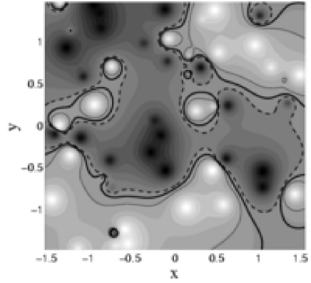
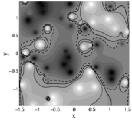
Figure 3: Profile of the disorder potential obtained from our Coulomb model on a $3.11\mu$m$\times 2.96\mu$m sample, without (upper panel) and with (lower panel) the $V^{\prime}({\bf r})$ correction at the $x=\pm L_{x}/2$ edges. The disorder potential varies between $-3$ meV and 3 meV, on a spatial length-scale much larger than $l=12.03$ nm. The critical region containing extended states is in the vicinity of $E=0.06$ meV. The contours are shown for $E=$0.0575 meV (dashed), 0.17 meV (thick solid) and 0.31 meV (thin solid). These energy values correspond to classical filling factors $\nu$=0.47, 0.58 and 0.68 in the upper panel and $\nu$=0.45, 0.56, 0.66 in the lower panel. The difference is due to the supplementary smooth potential $V^{\prime}$.

Figure 4: Semi-classical (dashed line) and quantum (solid line) filling factors for the disorder potential shown in Fig. 3, but different amplitudes of the triangular periodic potential (a) $A$=0; (b) $A$=0.05meV; (c) $A$=0.5meV and (d) $A$=5 meV. As expected, agreement exists only in the limit $A\rightarrow 0$.

Figure 5: Semi-classical (dashed line) and quantum (full line) density of states calculated from corresponding filling factors in Fig. 4. We show only the center of the disorder-broadened lowest Landau level, where the density of states is large.

For the first sample, we consider $\phi/\phi_{0}=3/2$ ($B=4.71$ T). The magnetic length is $l=12.03$ nm, and we choose a sample size $L_{x}=3.11\mu$m and $L_{y}=76a=2.964\mu$m. With these choices, the Landau level contains $N=10108$ states. The disorder potential obtained with our scheme described in Sec. III is shown in Fig. 3, both with and without the correction $V^{\prime}({\bf r})$. An extended equipotential line appears, as expected, at $\nu\approx 0.5$.

In Figs. 4 and 5 we plot the filling factor $\nu(E)$ and the corresponding total density of states $\rho(E)$ as a function of $E$ (computation details were given in Sec. IV.2.2). These quantities are obtained in the semi-classical limit (dashed line) and with the full, quantum-mechanical treatment (solid line). Results are shown for 4 different cases: (a) only disorder potential and (b, c, d) disorder plus a triangular periodic potential with amplitudes $A=0.05$, 0.5 and 5 meV, respectively. We only plot a relatively small energy interval where the DOS is significant, and ignore the asymptotic regions with long tails of localized states.

While the agreement between the semi-classical and quantum-mechanical treatment is excellent in the limit $A\rightarrow 0$, the two methods give more and more different results as the periodic potential amplitude is increased. As already explained, this is a consequence of the fact that the magnetic length $l$ is comparable to the lattice constant $a$, leading to a failure of the semi-classical treatment when this extra length-scale is introduced. In particular, in the case with the largest periodic potential [panel (d) of Figs. 4 and 5] we can clearly see the appearance of the 3 subbands expected for the Hofstadter butterfly at $\phi/\phi_{0}=3/2$, although the disorder leads to broadened and smooth peaks, and partially fills-in the gap between the lower two subbands. This picture [panel (d)] is quite similar to the density of states that Ref. MacDonald, calculated using the self-consistent Born approximation. This is expected since the SCBA approach is valid in the limit of strong periodic potential with weak disorder. However, the SCBA approach is not appropriate in the limit of moderate or strong disorder, where the higher order terms neglected in SCBA are no longer small. For disorder varying on a much longer length-scale than the periodic potential, one still expects that locally, on relative flat regions of disorder, the system exhibits the Hofstadter-type spectrum. However, these spectra are shifted with respect to one another by the different local disorder values. If disorder variations are small, then the total spectrum shows somewhat shifted subbands with partially filled-in gaps, but overall the Hofstadter structure is still recognizable. On the other hand, for moderate and large disorder, the detailed structure of the local density of states from various flat regions are hidden in the total density of states. All one sees are some broadened, weak peaks and gaps superimposed on a broad, continuous density of states.

We now analyze the nature of the electronic states for these configurations. We start with the case which has only disorder. In Fig. 6 we plot $|G^{R}(k_{\min},k_{\max};E)|^{2}$ as a function of the energy $E$, for different values of $\delta$ (computation details were given in Sec. IV.2.3). As already discussed, extended states are indicated by large values of this quantity, as well as a strong (roughly $1/\delta^{2}$) dependence on the value of the small parameter $\delta$.

Figure 6 reveals that as $\delta$ is reduced, resonant behavior appears in a narrow energy interval $E=0.02-0.36$ meV. Panel (a) shows that results corresponding to $\delta=10^{-7}$ eV and $\delta=10^{-8}$ eV indeed differ by roughly 2 orders of magnitude, with $\delta=10^{-8}$ eV showing sharper resonance peaks. The difference between results for $\delta=10^{-8}$ eV and $\delta=10^{-9}$ eV shown in panel (b), is no longer so definite. The reason is simply that for such small $\delta$, the denominator in the Green’s function expression is usually limited by $|E-E_{n,\alpha,\sigma}|$ and not by $\delta$ [see Eq. (12)], and the dependence on $\delta$ is minimal. Only if $E$ is such that $|E-E_{n,\alpha,\sigma}|<\delta$ can we expect to see a $\delta$ dependence, and indeed this is observed at some energies. Finally, in panel (c) we show the comparison with a larger energy interval. The value of the Green’s function decreases exponentially fast on both sides of the critical region, indicating strongly localized states. Here, data for $\delta=10^{-6}$ eV is a smooth curve, whose magnitude is much less than that of the other three values even for localized states. This is due to the fact that this $\delta$ is larger than typical level spacings. As a result, several levels contribute significantly to Green’s function at each $E$ value, and the destructive interference of the random phases of different eigenfunctions lead to the supplementary $\delta$-dependence. We conclude that the disorder potential has a critical energy regime of approximately $0.3$ meV width, covering less than 5% (in energy) and 20% (in number of states) of the disorder-broadened band with total width $\sim 6$ meV. The position of the critical energy interval is in agreement with the semi-classical results which suggest an extended state in the vicinity of $E=0.06$meV. By comparison with Fig. 4, we can also see that this critical regime corresponds to a roughly half-filled band, in agreement with the experiment.

The effect of an additional triangular periodic potential is shown in Fig. 7, where we plot the same quantity shown in Fig. 6 for a fixed $\delta=10^{-7}$ eV and different amplitudes $A=0$, 0.05, 0.5 and 5 meV, respectively. These results correspond to a different Coulomb disorder potential (not shown), as can be seen from the different location of its extended states. Here we see how the narrow critical interval of extended states grows gradually as the amplitude of periodic potential is increased and finally exhibits the three well-separated extended subbands expected for $\phi/\phi_{0}=3/2$ in the limit of vanishing disorder. The three subbands can already be resolved for the moderate case $A=0.5~{}$meV, although they are very wide and exhibit significant overlap.

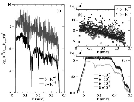
Figure 6: Semi-log plot of the amplitude of Green’s function matrix element between the two edge states near $x=\pm L_{x}/2$, as a function of energy. Only the disorder potential of Fig. 3 is present. (a) comparison between $\delta=10^{-7}$ and $\delta=10^{-8}$ results; (b) comparison between $\delta=10^{-8}$ and $\delta=10^{-9}$ results; (c) comparison between results corresponding to $\delta=\delta=10^{-6},10^{-7},10^{-8}$ and $10^{-9}$. (the last three curves are indistinguishable to the eye on this scale.) All $\delta$ values are in eV units.

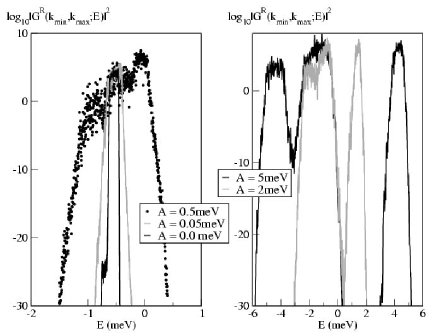
Figure 7: The effect of a triangular periodic potential on the critical energy regime. The disorder potential used here (not shown) supports a narrow interval of extended states centered at about $-0.6$ meV. As the amplitude $A$ of the periodic potential increases, the range of extended states increases dramatically. The left panel shows results for disorder-only and two relatively weak periodic potentials, while the right panel shows two larger periodic potentials where the three-subband structure expected for $\phi/\phi_{0}=3/2$ is clearly seen.

Qualitatively similar behavior is obtained if we use the Gaussian scatterers model for disorder. A typical realization of this disorder is shown in Fig. 8. Results for the Green’s function’s values with such disorder are shown in Fig. 9, for cases with pure disorder, and also cases with either a triangular or a square periodic potential. The magnetic field has been doubled, such that $\phi/\phi_{0}=3$. Similar to the case shown in Fig. 7, the periodic potential leads to a widening of the critical regime. For large periodic potentials, the expected Hofstadter-like three-subband structure emerges again. We conclude that Coulomb and Gaussian disorder models show qualitatively similar behavior.

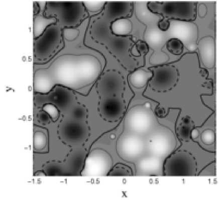
Figure 8: A disorder potential of Gaussian type on a roughly $3\mu m\times 3\mu m$ square. The three lines are equipotential contours close to the critical regime, with energies of -0.1 meV (dashed), 0 meV (thick solid) and 0.1 meV (thin solid). Cyclic boundary condition are applied in the $y$ direction.

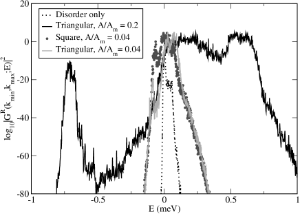
Figure 9: Green’s functions for a sample with Gaussian disorder and various periodic potentials. The calculation included 20216 states with $\phi/\phi_{0}=3$. Similar to results shown in Fig. 9, we see that the periodic potentials widen the critical region.

We now analyze the projected local density of states $\rho_{P}(E)$ discussed in Sec. IV.2.4, in order to understand the reason for this substantial widening of the critical region by even small periodic potentials. We consider a smaller sample, of size approximately $1.6\mu$m$\times 1.6\mu$m, and compute the projected density of states for 500 equally-spaced energy values, on a $60\times 60$ square grid and for a value $\delta=10^{-8}$ eV. This $\delta$ value is comparable or smaller than the level spacing, so we expect to see sharp resonances from the contribution of individual eigenfunctions as we scan the energy spectrum. Each computation generates a large amount of data (roughly 24M), corresponding to the 500 plots of the local density of states at the 500 values of $E$. Since we cannot show all this data, we select a couple of representative cases and some statistical data to interpret the overall results.

Figures 10 and 11 show some of our typical results. The two figures are calculated for the same Coulomb-disorder potential, for values of $E=-0.504$ meV (at the bottom of the band) and $E=-0.124$ meV (close to, but below the band center) respectively. Each figure contains four panels, panel (a) shows the profile of the disorder potential as well as an equipotential line (solid black) corresponding to the value $E$ considered; the other three panels show the projected density of states $\rho_{P}(E)$ for (b) pure disorder; (c) disorder plus triangular periodic potential with $A=0.1$ meV; (d) disorder plus square periodic potential with $A=0.1$ meV. In Fig. 10, this equipotential line (which traces the semi-classical trajectory of electrons with the same energy $E$)

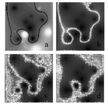
Figure 10: (color online) Projected local density of states $\rho_{P}({\bf r};E)$ for $E=-0.504$ meV. Panel (a) shows the profile of the disorder potential, and the equipotential contour (black line) corresponding to $E=-0.504$ eV. The other three panels show $\rho_{P}({\bf r};E)$ for (b) disorder only; (c) disorder plus triangular periodic potential with $A=0.1$ meV; (d) disorder plus square periodic potential with $A=0.1$ meV. The width and length of the sample are both $1.6\,\mu$m, and $\phi/\phi_{0}=3/2$. Increased brightness corresponds to larger values.

surrounds local minima of the disorder potential, suggesting localized electron states at such low energies. Indeed, this is what panels (b), (c) and (d) show. The projected density of states $\rho_{P}(E)$ is large (bright color) at the positions where electrons of energy $E$ are found with large probabilities. For pure disorder, we observe only closed trajectories (localized states), whose shape is in excellent agreement with the semi-classical trajectory, as expected. If a moderate periodic potential is added, the wave-functions spread over a larger area, and nearby contours sometimes merge together. Instead of sharp lines, as seen in panel (b), the contours now show clear evidence of interference effects of the wave-functions on the periodic potential decorating the electron reservoirs. Some periodic modulations can also be observed in the background of panels (c) and (d), especially for the square potential. These are not the direct oscillations of the periodic potentials, since the grid we use to compute these figures has a linear size equal to $7/10$ of the period $a=39$ nm of the periodic potential. Capturing detailed behavior inside each unit cell would require a much smaller grid, which is not only time consuming, but also violates the requirement that the grid size be of order $l$ or larger.

Figure 11 for an energy close to the band center, shows the same characteristics. For pure disorder, the electrons at this energy trace a sharp contour very similar

Figure 11: (color online) The same as in Fig. 10, but for an energy $E=-0.124$ meV close to the band center.

to the corresponding equipotential line shown in panel (a). Electrons are still not delocalized, since this contour does not connect either pair of opposite edges. However, addition of the periodic potential now leads to extended states for both types of periodic potentials [(c) and (d)] at roughly $E=-0.124$ meV, demonstrating the widening of the critical region with the addition of a periodic potential.

Physically, one can understand this spread of the wave function in the presence of the periodic potential using the semi-classical picture.Sorin If only a smooth disorder potential is present, the equipotential at any energy $E$ must be a smooth, continuous line. However, if a periodic potential with minima $-V_{m}$ and maxima $V_{M}$ is superimposed over disorder, the new equipotential line now breaks into a series of small “bubbles” surrounding the disorder-only contour. This happens throughout the area defined by the equipotentials $E-V_{M}$ and $E+V_{m}$ of the disorder potential, since the addition of the periodic potential leads new regions in this area to have a total energy $E$. Quantum mechanically, we expect some tunneling inside this wider area and this is indeed what we observe in Figs. 10 and 11. This mechanism suggests enhanced delocalization on both sides of the critical region as localized wave functions spread out over larger areas, as well as a widening of the critical region itself, in agreement with our numerical results.

This spreading of the wave functions in the presence of the periodic potential can also be characterized by counting, at a given energy $E$, the number of grid points ${\bf r}$ which have a value $\rho_{P}({\bf r};E)>\rho_{c}$, where $\rho_{c}$ is some threshold value. For sufficiently large $\rho_{c}$, this procedure counts grid points where electrons with energy $E$ are found with large probabilities, thus, in effect it characterizes the “spatial extent” of the wave functions.

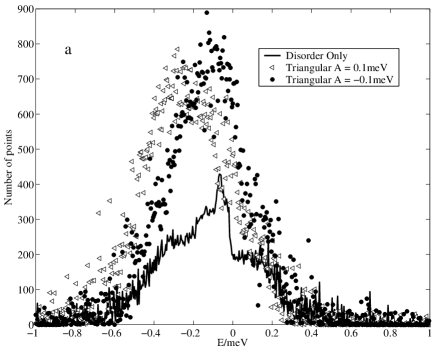
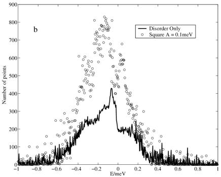
Figure 12: Number of grid points for which $\rho_{P}({\bf r},E)>100$ as a function of the energy $E$. This quantity characterizes the “spatial extent” of the wave function. The upper panel compares results for disorder only (A=0) and disorder plus triangular potentials with $A\pm 0.01$ meV. The difference observed for the two signs is a consequence of particle-hole asymmetry of the triangular potential. The lower panel shows results for disorder only and disorder plus a square potential.

The results of such counting are shown in Fig. 12 for 500 energy values corresponding to the disorder potential analyzed in Figs. 10 and 11. There are a total of $60\times 60=3600$ grid points on the sample. For the case of pure disorder (black line) we see that the largest values are found at energies just below 0, where the extended states (the critical region) are found for this particular realization of disorder. Because it is a smooth, sharp line, even the most extended trajectory has significant probabilities at only about 10% of the grid sites. For both higher and lower energies, this number decreases very fast, indicating wave functions localized more and more about maxima or minima of the disorder potential, as expected. Addition of a small periodic potential increases this number substantially, clearly showing the supplementary spreading of the wave functions in the presence of the periodic potential.

Figure 12 shows this effect for three types of periodic potential: triangular lattices with $A>0$ and $A<0$ (upper panel), and square lattice in the lower panel. All three cases show significant enhancement, as compared to the pure disorder case. In addition, we see that while the square potential gives a fairly symmetrical enhancement, the triangular potential does not, with curves for $\pm A$ not overlapping. This is a consequence of the asymmetric shape of the periodic potential, which has different values for its minima and maxima $|V_{m}|\neq|V_{M}|$, as well as different arrangements for the points where minima/maxima appear (triangular lattice vs. honeycomb lattice). Fig. 12 clearly shows that $A>0$ favors increased delocalization below the critical energy regime, while $A<0$ favors increased delocalization above it.

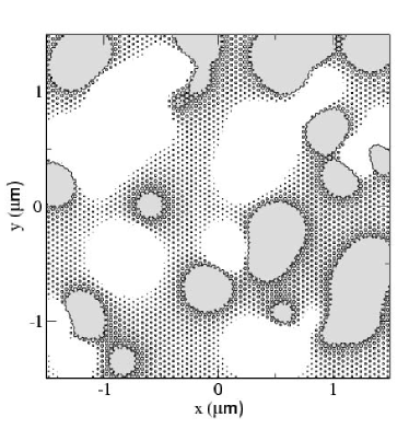
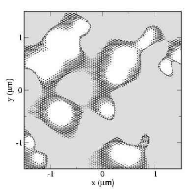
Figure 13: Equipotential contours at filling factor $\nu=0.3$ (upper panel) and $\nu=0.7$ (lower panel) for a $3\mu m\times 3\mu m$ sample with disorder plus a small triangular periodic potential with $A>0$. The shaded regions correspond to energies below the respective equipotential. In the semi-classical approximation, the shaded areas are filled with electrons, with the maximum density of $1/2\pi l^{2}$, whereas the white areas are completely devoid of electrons. Quantum-mechanically, one expects interference in the regions with small periodic “bubbles”, induced by the periodic potential (see Figs. 10 and 11).

The reason for this different response to the two signs of the triangular potential can be nicely explained within the semi-classical framework. In Fig. 13 we show the equipotential lines corresponding to filling factors $\nu=0.3$ (well below critical region) and $\nu=0.7$ (well above the critical region) for a realization of Coulomb disorder (not shown) plus a triangular potential with $A>0$. Areas with energy below the equipotential value are shaded. In this case we can clearly see that instead of the continuous, smooth trajectory expected for disorder-only cases, there are also extra “bubbles” regions connecting the areas between such contours. Since the choice $A>0$ leads to deep minima at $-V_{m}=-6A$ with triangular arrangement and relatively flat maxima at $+V_{M}=3A$ with honeycomb arrangement [see Eq. (6)], it follows that the triangular (honeycomb) “bubbles” region appear roughly in the area bounded by the equipotentials $E$ and $E+V_{m}$ (respectively, $E-V_{M}$ and $E$) of the pure disorder potential. At low filling factors, the pure disorder $E$ equipotential is a collection of closed contours surrounding local minima [see panel (d) of Fig. 10 for an illustration]. It follows that for the choice $V_{m}>V_{M}$, the more extended region with triangular “bubbles” will be found outside these “islands” and will lead to a spread of the wave function over considerably larger areas, as indeed seen in the upper panel of Fig. 13. On the other hand, at large filling factors the disorder-only contours are “islands” surrounding the maxima of the disorder potential. In this case, contours between $E$ and $E+V_{m}$ are inside the $E$ contour, so the triangular “bubbles” region does not help to connect various “islands” as before. The honeycomb “bubbles” regions does this, but because $V_{M}<V_{m}$ the extension of the wave function between “islands” is significantly smaller in this case.

In the quantum-mechanical case one expects interference (due to tunneling) effects between the small “bubbles” regions, and therefore a wave function which is extended over their entire area, as indeed we observe to be the case in Figs. 10 and 11. In other words, one expects that a triangular potential with $A>0$ will lead to considerable increase of the localization length, and respectively widening of the critical energy region, at filling factors below one-half, whereas $A<0$ will favor delocalization at filling factors above one-half, as seen in Fig. 12. This asymmetry is therefore clearly a consequence of the asymmetry of the triangular potential, and is absent for a square potential with only lowest order Fourier coefficients, which possesses electron-hole symmetry. This should have clear implications for the transport properties of the system.

VI Summary and Conclusions

In this study we have investigated the effects of moderate-to-large smooth disorder on the Hofstadter butterfly expected for 2DES in a perpendicular magnetic field and a pure periodic modulation. The parameters of our study are chosen so as to be suitable for the interpretation of recent experiments on a two dimensional electron system in GaAs/AlGaAs heterostructure with periodic modulation provided by a diblock copolymer, Sorin The experiment shows that (i) the longitudinal resistance $R_{xx}$ is still peaked approximately at half filling; (ii) there are many reproducible oscillations in $R_{xx}$, indicating non-trivial electronic structures in the patterned sample; (iii) the distribution of these oscillatory features is asymmetric, with most of them appearing on the high magnetic fields (i.e. low filling factors $\nu<0.5$) side of the peak of $R_{xx}$; and (iv) the temperature dependence of $R_{xx}$ indicates that the asymmetric off-peak resistance is thermally excited, whereas the central $R_{xx}$ peak (close to half filling) has metallic behavior.

These observations cannot be explained on the basis of the Hofstadter structure.Sorin This is not surprising, since one expects that large disorder will modify this structure considerably. Effects of small disorder on the Hofstadter butterfly had been investigated previously using SCBA,MacDonald but this basically perturbational approach is not appropriate for the case of moderate-to-large smooth disorder. Instead, we identify and use a number of techniques which give the exact solution (if electron-electron interactions, as well as inelastic scattering are neglected) while avoiding brute force numerical diagonalizations.

Our results demonstrate that while the Hofstadter butterfly is destroyed by large disorder, the effects of the periodic potential are non-trivial for states near the critical regime. Firstly, they lead to a significant increase in localization lengths of the localized states at mesoscopic ($\mu m$) length scale and induce an effective widening of the critical regime near the critical regime. This is achieved through a spreading of the electron wave-function on the flat regions of the slowly varying disorder potential, where their behavior is dominated by the periodic modulation. This regime shows an interesting transition between the pure disorder and the pure periodic potential cases. In the case of pure disorder, the semi-classical approach tells us that at finite filling factors, some areas of the sample are fully occupied by electrons with the maximum possible density of $1/(2\pi l^{2})$ (these are the areas where the disorder potential has minima) whereas other areas are fully devoid of electrons (areas where the potential has maxima) and the boundary between such regions is very sharp. On the other hand, for a pure periodic modulation all wave functions have translational invariance with the proper symmetry, and therefore electron densities are uniform over the entire sample (up to small periodic modulations inside each unit cell).

When both types of potential are present, with disorder being dominant, our results show three types of areas. There are regions which are fully occupied and regions which are completely devoid of electrons, as in the case of pure disorder. However, the periodic potential leads to a widening of the boundary between the two, where the wave functions interact with several oscillations of the periodic modulation and therefore have some partial local filling. As the critical regime containing wave functions percolating throughout the sample is approached, this spreading of the wave function becomes dominant in establishing the transport properties of the system.

An equivalent way to say this is that the main effect of the periodic potential is to provide bridging between the fully-occupied electron “puddles” created by the disorder potential. Since the connecting areas are relatively flat, the local wave functions respond to the local periodic potential, and therefore locally have a Hofstadter-butterfly like structure. If the partial filling factor in such a region is inside the gap of the local Hofstadter butterfly structure, one expects no transport through this local area. This should result in a dip in the longitudinal transport, since in such cases the periodic potential will not transport electrons from one “puddle” to another one. By contrast, if the local filling factor in such a region is inside a subband of a local Hofstadter structure, this area will establish a link between different “puddles” and thus help enhance the transport through the sample. Transport in this regime should show strong thermal activated behavior, in contrast to metallic transport in the critical regime where the wave functions connect opposite edges of the sample.

As a result, one expects a series of local minima and maxima in the longitudinal resistivity on either side of the central peak induced by the extended states (critical regime). Furthermore, for an asymmetric triangular potential, this response should be strongly asymmetric, with the effect most visible on one side of the central peak. (One must keep in mind that since tunneling leads to exponential dependencies, even small differences in the extent of the wave functions can have rather large effects on $\rho_{xx}$). Such an asymmetry should also be present in longitudinal conductance of finite but low temperature, e. g. in the hopping regime which is sensitively dependent on the nature of the localized wavefunctions, as is indeed seen experimentally.Sorin

To summarize, our qualitative explanation for the various experimental features are as follows:

(i) The $R_{xx}$ peak is roughly at the center of the band because the weak periodic potential cannot establish a Hofstadter-like structure over the whole band. Instead, low and high $\nu$ states are strongly localized and do not transport longitudinal currents.

(ii) New extended states induced by the periodic potential are responsible for the reproducible peaks and valleys appearing in $R_{xx}$.

(iii) The periodic potential also leads to the expansion of localized wave functions, which contribute to the thermally activated conduction at lower filling factors. The detailed structure of the wave functions gives rise to the oscillations of the off-peak $R_{xx}$, similar to conductance fluctuations.Shayegan Finally,

(iv) the asymmetry in $R_{xx}$ is a manifestation of the asymmetry of the triangular potential, which has a stronger effect at low filling factors than at high filling factors for $A>0$. We predict that this asymmetry should be absent for a symmetric square periodic potential.

The weak point in our calculation is that we are unable to accurately model the potential in the real samples, because various screening effects have not been properly taken into account. Also, we have no quantitative information about the magnitude of the periodic potential in the 2DES layer, because of the additional strainLarkin contribution induced by the periodic decoration. As a result, we only claim qualitative agreement with the experiment, although our investigations show the same type of behavior for various types of disorder potentials and various (small-to-moderate) strengths of the periodic potential. The most direct check of this work would be an experimental demonstration that thermally activated conduction appears symmetrically on both sides of the $R_{xx}$ peak for a periodic potential with square symmetry and primarily lowest Fourier coefficients.

Limited computer resources restrict our calculations to samples no larger than $3\mu$m$\times 3\mu$m, while the sample used in experiment has a size of $20\mu$m$\times 20\mu$m. From a theoretical point of view, it is interesting to ask what is the thermodynamic limit. For pure disorder, it is believed that in this limit the typical size of wavefunction diverges at a single critical energy. Since we cannot pursue size-dependent analysis for samples larger than $3\mu$m$\times 3\mu$m, we do not know whether the small periodic potential will lead to a finite size critical regime in the thermodynamic limit, although this seems likely. From an experimental point of view, the interesting question is whether the Hofstadter structure can be observed at all. Our studies suggest that this may be possible for small mesoscopic samples, where the slowly-varying disorder has less effect. Alternatively, one must find a way to boost the strength of the periodic modulations inside the 2DES.

References

- (1) K. von Klitzing, G. Dora and M. Pepper, Phys. Rev. Lett. 45, 494 (1980).
- (2) D. C. Tsui, H. L. Strmer, and A. C. Gossard, Phys. Rev. Lett. 48, 1559 (1982).
- (3) For a review, see “The Quantum Hall Effect”, edited by R.E. Prange and S.M. Girvin, Graduate Texts in Contemporary Physics (Springer-Verlag, New York, 1987).
- (4) D. R. Hofstadter, Phys. Rev. B 14, 2239 (1976).
- (5) Dieter Langbein, Phys. Rev. 180, 633 (1969); the electronic structure in the asymptotic cases is periodic in or , and the equality is meant modulo this periodicity.
- (6) D. Springsguth, R. Ketzmerick, and T. Geisel, Phys. Rev. B 56, 2036 (1997).
- (7) T. Schlösser, K. Ensslin, J. P. Kottahaus and M. Holland, Europhys. Lett. 33, 683 (1996).
- (8) D. Weiss, M. L. Roukes, A. Menschig, P. Grambow, K. von Klitzing and G. Weimann, Phys. Rev. Lett. 66, 2790 (1991).
- (9) C. Albrecht, J. H. Smet, K. von Klitzing, D. Weiss, V. Umansky and H. Schweizer, Phys. Rev. Lett. 86, 147 (2001).
- (10) Rolf R. Gerhardts, Dieter Weiss and Ulrich Wulf, Phys. Rev. B 43, 5192 (1991).
- (11) S. Melinte, M. Berciu, C. Zhou, E. Tutuc, S. J. Papadakis, C. Harisson, E. P. De Poortere, M. Wu, P. M. Chaikin, M. Shayegan, R. N. Bhatt and R. A. Register, to appear in Phys. Rev. Lett. (cond-mat/0311400).
- (12) S. Melinte, E. Grivei, V. Bayot, and M. Shayegan, Phys. Rev. Lett. 82, 2764 (1999), and references therein.
- (13) P. Chaikin (private communication).
- (14) U. Wulf and A. H. MacDonald, Phys. Rev. B 47, 6566 (1993).
- (15) B. Huckstein and R. N. Bhatt, Surface Science 305, 438 (1994).
- (16) F.H. Claro and G.H. Wannier, Phys. Rev. B 19, 6068 (1979).
- (17) D. Springsguth, R. Ketzmerick, and T. Geisel, Phys. Rev. B 56, 2036, (1997).
- (18) D. Pfannkuche and R. R. Gerhardts, Phys. Rev. B 46, 12606 (1992).
- (19) S. A. Trugman, Phys. Rev. B 27, 7539 (1983).
- (20) John A. Nixon and John H. Davies, Phys. Rev. B 41, 7929 (1990).
- (21) M. Stopa, Phys. Rev. B 53, 9595 (1996); Physica B 227, 61 (1996).
- (22) S. Das Sarma and S. Kodiyalam, Semiconductor Science and Technology 13, A59 (1998).
- (23) T. Ando, J. Phys. Soc. Japan 53, 3101 (1984).
- (24) Ralph Williams, “Modern GaAs Processing Methods”, (Artech House Publishers, BostonLondon, 1990).
- (25) B. I. Halperin, Phys. Rev. B 25, 2185 (1982).
- (26) Allowed trajectories are such that the total flux through the area enclosed by the trajectory is an integer number of elementary fluxes . This can be understood in the spirit of the Bohr-Sommerfeld quantization rule, since it ensures constructive interference of the wave function around the contour. Except for the most localized states, found at the bottom and the top of the band, all other localized states are such that they enclose large numbers of magnetic fluxes. Imposing the exact quantization condition (which is numerically time consuming) leads to a negligible change in the value of the allowed equipotential value with respect to a randomly chosen value. Since such small changes do not influence the shape of the density of states, we ignore imposing this quantization condition in obtaining the semi-classical densities of states.
- (27) we use the package FFTW2.1.3 available on-line at http://www.fftw.org.
- (28) Chenggang Zhou and R. N. Bhatt, Phys. Rev. B 68, 045101 (2003).
- (29) Xiaoye S. Li, M. Baertschy, T. N. Rescigno, W. A. Issacs and C. W. McCurdy, Phys. Rev. A 63, 022712 (2001). Details regarding the software also available at http://www.nersc.gov/ xiaoye/SuperLU.
- (30) Roger Haydock, Phys. Rev. B 61, 7953 (2000).
- (31) J. A. Simmons, H. P. Wei, L. W. Engel, D. C. Tsui and M. Shayegan, Phys. Rev. Lett. 63, 1731 (1989).
- (32) J. H. Davies and I. A. Larkin, Phys. Rev. B 49, 4800 (1994).