Thermopower induced by a supercurrent in superconductor-normal-metal structures

Abstract

We examine the thermopower $Q$ of a mesoscopic normal-metal (N) wire in contact to superconducting (S) segments and show that even with electron-hole symmetry, $Q$ may become finite due to the presence of supercurrents. Moreover, we show how the dominant part of $Q$ can be directly related to the equilibrium supercurrents in the structure. In general, a finite thermopower appears both between the N reservoirs and the superconductors, and between the N reservoirs themselves. The latter, however, strongly depends on the geometrical symmetry of the structure.

Thermoelectric effects in electrical conductors typically result from the asymmetry of the Fermi sea between the electron ($E>E_{F}$) and hole-like ($E<E_{F}$) quasiparticles. This is illustrated by the Mott relation Ashcroft and Mermin (1967) for the thermopower

$$Q\equiv\left.\frac{\Delta V}{\Delta T}\right|_{I=0}=-\frac{\pi^{2}}{3}\,\frac{k_{B}^{2}T}{e}\,\left.\frac{\mathrm{d}\ln{\sigma(E)}}{\mathrm{d}E}\right|_{E=E_{F}}\,.$$ (1)

This relates the potential difference $\Delta V$ generated by the temperature difference $\Delta T$ to the energy dependence of the conductivity $\sigma$ due to the asymmetry above and below the Fermi sea.

In metals, the electron-hole asymmetry is governed by the parameter $k_{B}T/E_{F}$ arising from the next-to-leading term in the Sommerfeld expansion. At sub-Kelvin temperatures, this leads to a very small $Q$, typically below 10 nV/K. However, recent experiments Eom et al. (1998); Dikin et al. (2002); Parsons et al. (2003) measuring the thermopower in normal-metal wires connected to superconducting electrodes indicate that it exceeds this prediction at least by an order of magnitude, and, moreover, show that $Q$ oscillates with the phase difference between the two superconducting contacts.

Mott relation is expected to fail in the presence of the superconducting proximity effect when the geometrical symmetry in the measured sample is broken Heikkilä et al. (2000). Our aim is to show that with nearby superconductors, normal-metal circuits can show a thermoelectric effect independent of electron–hole-symmetries, since the proximity effect couples the temperatures to the potentials through the supercurrent. This effect is at least two orders of magnitude larger than that predicted by Eq. (1) (c.f. Fig. 1).

We discuss the system shown in the inset of Fig. 2, with a supercurrent flowing between the two superconducting elements. Our main result (Eq. (8)) states that the thermopower $Q_{\mathrm{NS}}$ between the N and S parts of the structure is proportional to the difference in the supercurrents at the temperatures $T_{1}$, $T_{2}$ of the two N electrodes. Moreover, we obtain a similar result (Eq. (10)) for the thermopower $Q_{\mathrm{NN}}$ between the normal parts in a geometrically asymmetric structure. This can be understood phenomenologically as follows. If $T_{1}\neq T_{2}$, the temperature-dependent Dubos et al. (2001) equilibrium supercurrent $I_{S}(T_{1})$ in wire 3 is different from $I_{S}(T_{2})$ in wire 4. (For this qualitative picture, we approximate these wires to be at the temperatures $T_{1}$, $T_{2}$.) Thus, a compensating effect must arise to guarantee the conservation of currents. Should the N reservoirs be kept at the same potential as the superconductors, a quasiparticle current $I_{\text{qp}}\propto(I_{S}(T_{1})-I_{S}(T_{2}))$ from them to the superconductors would balance the difference. However, when no current is allowed to flow in wires 1 and 2, a compensating N–S potential difference $V_{N}-V_{S}\propto R(I_{S}(T_{1})-I_{S}(T_{2}))$ is induced instead. The induced potentials oscillate with phase differences, similarly to the supercurrent, and may differ in the two N reservoirs, especially in asymmetric structures.

In the following, we concentrate on the diffusive limit, and model the setup with the Keldysh-Usadel equations Belzig et al. (1999). These equations assume electron-hole symmetry, under which Eq. (1) predicts a vanishing $Q$.

The Keldysh-Usadel equations are formulated in terms of the quasiclassical Green’s functions (which are matrices in the Keldysh-Nambu space), but here we use their $\theta$-parametrization Belzig et al. (1999), for convenience. It reduces the problem to two sets of equations, the spectral equations and the kinetic equations. In terms of the parameterizing functions $\chi$ and $\theta$, the phase and the proximity effect strength, the spectral equations in normal metals are

$$D\nabla^{2}\theta=-2iE\sinh(\theta)+\frac{1}{2}D(\nabla\chi)^{2}\sinh(2\theta)\,,$$ (2a)

$$D\nabla\cdot j_{E}=0,\quad j_{E}\equiv-\sinh^{2}(\theta)\nabla\chi\,.$$ (2b)

Here, the factor $D$ is the diffusion constant of the normal metal, and $E$ is the energy with respect to the superconductor potential. The kinetic equations are expressed using the symmetric and antisymmetric parts, $f_{T}$ and $f_{L}$ Belzig et al. (1999), of the electron distribution function $f(E,\vec{r})$:

$$D\nabla\cdot j_{L} =0, j_{L} \equiv\mathcal{D}_{L}\nabla f_{L}-\mathcal{T}\nabla f_{T}+j_{S}f_{T}\,,$$ (3a)

$$D\nabla\cdot j_{T} =0, j_{T} \equiv\mathcal{D}_{T}\nabla f_{T}+\mathcal{T}\nabla f_{L}+j_{S}f_{L}\,.$$ (3b)

The equations imply that the spectral current densities $j_{L}$ and $j_{T}$ are conserved (we neglect inelastic scattering). Thus the observable charge and energy current densities,

$$j_{c}=\frac{\sigma^{N}}{2e}\int j_{T}\mathrm{d}E\quad\text{and}\quad j_{Q}=\frac{\sigma^{N}}{2e^{2}}\int Ej_{L}\mathrm{d}E\,,$$ (4)

are also conserved.

The coefficients $\mathcal{D}_{L}$, $\mathcal{D}_{T}$, $\mathcal{T}$ and $j_{S}$ appearing in the kinetic equations are obtained from the spectral equations:

$$\!\!\mathcal{D}_{L/T}\equiv\frac{1}{2}\left(1+|\cosh\theta|^{2}\mp|\sinh\theta|^{2}\cosh(2\text{Im}[\chi])\right),$$ (5a)

$$\mathcal{T}\equiv\frac{1}{2}|\sinh\theta|^{2}\sinh(2\text{Im}[\chi]),\quad j_{S}\equiv\text{Im}[j_{E}].$$ (5b)

Here, $\mathcal{D}_{L}$ and $\mathcal{D}_{T}$ are the local spectral energy and charge conductivities, and $j_{S}$ is the spectral density of the supercurrent Heikkilä et al. (2002). The factor $\mathcal{T}$ arises in the formalism and has an effect on the thermopower. The normal-state values of these coefficients are $\mathcal{D}_{L}=\mathcal{D}_{T}=1$ and $j_{S}=\mathcal{T}=0$.

At nodes of wires, assuming clean metallic contacts, the functions $\theta$, $\chi$ and $f$ are continuous and Kirchoff-like “spectral current conservation laws” Nazarov (1999) imply that $A\sigma^{N}j_{L/T}$ and $A\sigma^{N}j_{S}$ are conserved. Here, $A$ is the cross-sectional area of a wire and $\sigma^{N}$ the normal-state conductivity. At clean metallic reservoir contacts most of the functions get their bulk values Belzig et al. (1999). However, for energies below the superconducting energy gap $\Delta$, the valid boundary conditions at superconductor interfaces are $j_{L}=0$, prohibiting the energy flow, and $f_{T}=0$, assuming no charge imbalance in the superconductors.

The coefficients $j_{S}$ and $\mathcal{T}$ couple the energy and charge currents together, and give rise to a finite thermopower. Moreover, these coefficients oscillate with the phase difference in the system, and thus the value of the thermopower should also oscillate. When there is no phase difference, $\mathcal{T}=j_{S}=0$, and the thermopower vanishes.

The energy scale of temperatures and potentials is specified by the Thouless energy

$$E_{T}\equiv\frac{\hbar D}{L^{2}}\approx\left\{\begin{array}[]{cc}13~{}\mu\text{V}&\;e\\ 0.15~{}\text{K}&\;k_{B}\end{array}\right\}\;\frac{D/(200~{}\mathrm{\frac{cm^{2}}{s}})}{(L/\mathrm{\mu{}m})^{2}}\,,$$ (6)

corresponding to a wire of length $L$ Heikkilä et al. (2002). Moreover, $E_{T}$ of the link between the superconductors is a natural energy scale for the spectral equations. As long as $E_{T}\!\ll\!\Delta$, the results can be scaled to fit all systems with similar ratios of wire lengths and areas.

Since there are no general analytical solutions to the problem, we solve the spectral equations numerically, and make a few approximations to solve the kinetic equations. However, the data shown in the figures is obtained numerically without any approximations.

First, we note that the “local potential” $f_{T}$ is generally small (as shown by the numerical results), as are the induced potentials at the reservoirs. Thus, we can neglect the terms proportional to it in the kinetic equation (3a). Physically this means that we mainly neglect the effect of supercurrent on the energy currents and the temperatures. (If the potentials were large, the omitted term would be the source for a Peltier-like effect Heikkilä et al. (2003).) With this approximation, we integrate the kinetic equations, which yields the connection between the spectral current densities and the distribution functions $f_{L}(x)$ and $f_{T}(x)$ at the ends of a wire of length $L$:

$$j_{L} =\frac{1}{LM_{L}}\,(f_{L}(L)-f_{L}(0))\,,$$ (7a)

$$j_{T} =\frac{1}{LM_{T}}\,(f_{T}(L)-f_{T}(0))+j_{S}f_{L}(0)$$ (7b)

$$+\frac{1}{L^{2}M_{L}M_{T}}\!\left(\int_{{0}}^{L}\!\!\!\frac{\mathcal{T}}{\mathcal{D}_{L}\mathcal{D}_{T}}\mathrm{d}x+j_{S}\int_{0}^{L}\!\!\!\int_{0}^{x}\!\!\!\frac{\mathrm{d}x^{\prime}\mathrm{d}x}{\mathcal{D}_{L}(x^{\prime})\mathcal{D}_{T}(x)}\right)$$

$$\quad\times(f_{L}(L)-f_{L}(0))\,.$$

Here $M_{L/T}\equiv\frac{1}{L}\int_{0}^{L}\mathcal{D}_{L/T}^{-1}\,\mathrm{d}x$ are the dimensionless spectral energy and charge resistances. To simplify the final result, we also approximate $\mathcal{D}_{L}=1$ in (7), and $\mathcal{D}_{T}=1$ in the latter term in (7b), since the variation in $\mathcal{D}_{L}$ (away from superconductor interfaces) and $\mathcal{D}_{T}$ with respect to the energy is smaller than that of the other coefficients. Numerical results verify that this does not affect the result crucially. The energy-dependent $1/M_{T}$ as a coefficient for $f_{T}$ causes an important temperature dependence of the conductance, so we retain it.

Using Eqs. (7) and the conservation of spectral currents, we obtain a linear system of equations for the spectral current densities. They can be solved with respect to the given temperatures and potentials in the reservoirs, with different results for $|E|<\Delta$ and $|E|>\Delta$, due to the different boundary conditions. Next, we integrate over the energy to obtain the observable current densities, after which we require the condition $j_{c,1}=j_{c,2}=0$. To solve the resulting equations for the small induced potentials $eV_{1}$ and $eV_{2}$, we linearize the distribution functions with respect to them, and obtain a linear equation for the potentials, which can then be solved.

If we proceed with the analytical approximation in the limit $\Delta\gg E_{T},eV,k_{B}T$ by neglecting $\mathcal{T}$ and the energy dependence of $\mathcal{D}_{T}$, we obtain the dominant term:

$$\begin{split}V_{1/2}^{0}=\frac{1}{2}\frac{R_{5}(2R_{4/3}+R_{5})\;\;R_{3/4}(I_{S}(T_{1})-I_{S}(T_{2}))}{(R_{1}+R_{2}+R_{5})(R_{3}+R_{4}+R_{5})}\,.\end{split}$$ (8)

Here, $I_{S}(T)=(A\sigma^{N}/e)\int_{{0}}^{\infty}j_{S}f_{L}^{0}\mathrm{d}E$ is the observable equilibrium supercurrent flowing in the system when all parts are at the temperature $T$ and there are no potential differences. Moreover, $f_{L,k}^{0}\equiv\tanh\left(E/(2k_{B}T_{k})\right)$ is a linearized distribution function, and $R_{k}=L_{k}/(A_{k}\sigma^{N}_{k})$ are the normal-state resistances of the wires. Thus a difference in equilibrium supercurrents due to the varying $f_{L}$ contributes significantly to the thermopower.

Similarly, we can take the effect of $\mathcal{T}$ into account and obtain the correction terms

$$eV_{1/2}^{1} =\frac{\mp R_{1/2}}{R_{1}+R_{2}+R_{5}}\,\int_{{0}}^{\infty}\!\!\!\left(f_{L,1}^{0}-f_{L,2}^{0}\right)\left<\mathcal{T}_{1/2}\right>\,\mathrm{d}E$$ (9)

$$\mp\frac{R_{3/4}R_{5}}{(R_{1}+R_{2}+R_{5})R_{SNS}}\int_{{0}}^{\infty}\!\!\!\left(f_{L,1}^{0}-f_{L,2}^{0}\right)\left<\mathcal{T}_{5}\right>\,\mathrm{d}E\,,$$

where $R_{SNS}=R_{3}+R_{4}+R_{5}$. Here, we denoted $\left<\mathcal{T}_{k}\right>\equiv\frac{1}{L_{k}}\int_{{0}}^{L_{k}}\mathcal{T}_{k}\,\mathrm{d}x$ (shown in Fig. 3d compared with $j_{S}$). The correction is necessary, as it compensates for the fast decay of $V_{1/2}^{0}$ at high temperatures $k_{B}T\gtrsim 10~{}E_{T}$, but it is not negligible even at lower temperatures (see Fig. 2).

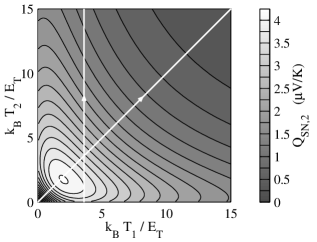
Figure 1: N–S thermopower at different temperatures $T_{1}$ and $T_{2}$ of the normal electrodes, for a setup with $L_{k}$ and $A_{k}$ assumed equal for all wires, and in the limit $\Delta\gg E_{T},eV,k_{B}T$. The analytical approximation (8) with $\mathcal{T}$-correction (9) deviates at worst $15\%$ from these results, but the difference is over 5% only where $Q_{\mathrm{NS}}$ is small, i.e. $k_{B}T_{1},k_{B}T_{2}\gtrsim 10~{}E_{T}$. In all of the figures, $E_{T}=\hbar D/(L_{3}+L_{4}+L_{5})^{2}$, and we plot the results for $\phi=\pi/2$ yielding a near-maximal supercurrent.

The induced $Q_{\mathrm{NS,2}}\equiv V_{2}/(T_{2}-T_{1})\approx Q_{\mathrm{NS,1}}$ is shown in Fig. 1. The magnitude of $Q_{\mathrm{NS}}$ is of the order $\sim\mathrm{\frac{\mu{}V}{K}}$ at highest, but there is also a strong temperature dependence. Figure 2 shows cross sections of Fig. 1, compared with the approximation (8).

We see that Eqs. (8) and (9) predict an induced N–N potential difference

$$\Delta V\equiv V_{2}-V_{1}\approx(V_{2}^{0}-V_{1}^{0})+(V_{2}^{1}-V_{1}^{1})\,.$$ (10)

In a left-right symmetric structure both terms vanish, but $Q_{\mathrm{NN}}$ may still be finite since $\mathcal{D}_{T}$ is energy-dependent:

$$\Delta V \approx\int_{{0}}^{\infty}\tilde{R}^{-1}\left(\frac{\operatorname{sech}^{2}\biglb(\frac{E}{2k_{B}T_{1}}\bigrb)}{2k_{B}T_{1}}-\frac{\operatorname{sech}^{2}\biglb(\frac{E}{2k_{B}T_{2}}\bigrb)}{2k_{B}T_{2}}\right)\mathrm{d}E$$

$$\qquad\times(R_{1}+(R_{3}R_{5})/(2R_{3}+R_{5}))(V_{1}^{0}+V_{1}^{1})\,,$$ (11)

valid for a symmetric structure $R_{1}\!=\!R_{2}$, $R_{3}\!=\!R_{4}$. Here the coefficient $\tilde{R}=\tilde{R}_{1}+(\tilde{R}_{3}\tilde{R}_{5})/(2\tilde{R}_{3}+\tilde{R}_{5})$, where $\tilde{R}_{k}=M_{T,k}R_{k}$ are the spectral resistances of the wires. The voltage (Thermopower induced by a supercurrent in superconductor-normal-metal structures) can be understood to be caused by the proximity-effect-induced temperature dependence of conductances Charlat et al. (1996), which creates asymmetry in resistances. However, in reality the asymmetry of the structure causes likely a more significant effect (see Fig. 4), especially at $T_{1}\approx T_{2}$, where Eq. (Thermopower induced by a supercurrent in superconductor-normal-metal structures) predicts $\Delta V\sim(T_{2}-T_{1})^{2}$ .

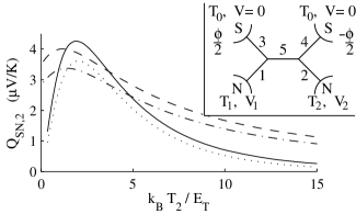
Figure 2: N–S thermopower along the cross sections of Fig. 1. Solid: $Q_{\mathrm{NS}}$ at $T_{1}\approx T_{2}$. Dotted: Approximation (8). The correction (9) accounts for most of the difference. Dashed: $Q_{\mathrm{NS}}$ at $k_{B}T_{1}=3.6~{}E_{T}$ with varying $T_{2}$. Dash-dotted: the corresponding approximation. Inset: The setup under consideration: two superconducting (S) reservoirs with phase difference $\phi$ connected to two normal-metal (N) reservoirs through diffusive normal-metal wires. We assume that the lengths $L_{k}$, $k=1,\ldots,5$ of the wires satisfy $\xi_{0}\lesssim L_{k}\ll l_{\phi},l_{E}$, where $\xi_{0}=\sqrt{\hbar D/(2\Delta)}$ is the superconducting coherence length, $l_{\phi}$ the phase-coherence length and $l_{E}$ the energy-relaxation length. We also consider the wires as quasi-1D structures Heikkilä et al. (2002).

Equation (8) implies that the thermopower should oscillate as a function of the phase difference $\phi$ between the two superconducting elements, because the equilibrium supercurrent oscillates roughly as $\sin(\phi)$. Numerical simulations show (see Fig. 3c) that also the exact solution oscillates similarly, vanishing at $\phi=0$.

Besides changing the prefactors in Eqs. (8,9), varying the resistances of the wires from the near-symmetric presented in the figures changes the behavior in the supercurrent Heikkilä et al. (2002) and the coefficient $\mathcal{T}$. In general, large departures from such symmetry decrease the potentials.

A finite value for $\Delta$ causes two distinct modifications to the thermopower. First, the coefficients (5) are modified, but changes are mostly only quantitative, e.g. sharpening of peaks (see Fig. 3a). Secondly, there is also a contribution from energies $E>\Delta$, which couples the superconductor temperature $T_{0}$ to the system. The latter effect is weaker than those predicted by Eqs. (8) and (9) at least for $\Delta>30~{}E_{T}$. Although the coupling of $T_{0}$ is weak, it induces finite potentials even for $T_{1}=T_{2}$ (Fig. 3b).

Our predictions agree quantitatively with the experimental results with the correct order of magnitude for both the linear thermopower Dikin et al. (2002) and the temperature scale Eom et al. (1998). The flux dependence (antisymmetric about $\phi=0$ — this holds for the exact as well as the approximate solutions) is in accord with most of the measurements in Eom et al. (1998); Dikin et al. (2002); Parsons et al. (2003). However, we cannot explain the symmetric oscillations with respect to zero flux, seen in the ”house” interferometers in Ref. Eom et al. (1998). Moreover, the main result, Eq. (8) cannot describe a sign reversal of $Q_{\mathrm{NS}}$ Parsons et al. (2003), but there is no principal reason forbidding such an effect in a suitable structure. Nevertheless, further experiments are required to quantitatively demonstrate the connection between the thermopower and the supercurrent.

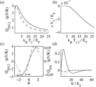
Figure 3: (a) N–S thermopower at $k_{B}T_{1}=3.6~{}E_{T}$ for various values of $\Delta$: $\infty$ (solid), $54~{}E_{T}$ (dotted), $27~{}E_{T}$ (dashed). Superconductor temperature $T_{0}=3.6~{}E_{T}$ is fixed. (b) Potential $eV_{2}$ induced due to the energies above $\Delta$, with $\Delta=27~{}E_{T}$. Here, $k_{B}T_{0}=3.6~{}E_{T}$ but $T_{1}=T_{2}$ vary. (c) Phase oscillation of $Q_{\mathrm{NS}}$ (solid) and $Q_{\mathrm{NN}}$ (dashed), at $k_{B}T_{1}=4.5~{}E_{T},\,k_{B}T_{2}=1.8~{}E_{T}$. Due to a numerical convergence problem, there is no data for $|\phi|>2.1$. (d) Spectral variables: $L_{3}j_{S}$ (solid), $\left<\mathcal{T}_{1}\right>$ (dashed), $\left<\mathcal{T}_{3}\right>$ (dotted). In each figure, all the lengths $L_{k}$ and areas $A_{k}$ are assumed equal.

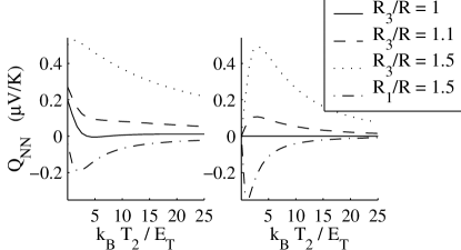
Figure 4: Left: N–N thermopower induced by setup asymmetry, at fixed $k_{B}T_{1}=3.6~{}E_{T}$. One wire (1 or 3) is assumed to have a different resistance than the others. Right: N–N thermopower with the same parameters, but with $T_{1}\approx T_{2}$.

Results of similar type as presented in this Letter for the N-S thermopower have been obtained for small temperature differences in Refs. Seviour and Volkov (2000); Kogan et al. (2002), assuming high tunnel barriers at the N-S contacts. However, the direct connection between the thermopower and the supercurrents as in Eq. (8) has not been shown. Moreover, Ref. Kogan et al. (2002) discusses a finite N–N thermopower from the energies above $\Delta$. Our results show that for an appreciable temperature difference between the N reservoirs, this effect is washed out by the asymmetry effects, at least for $\Delta\gtrsim 30E_{T}$.

In summary, we have obtained a relation linking the voltages induced by a temperature difference to the supercurrent in a mesoscopic structure. The phase-oscillating N–S thermopower is mostly induced by the temperature dependence in the supercurrent, and the N–N thermopower can be attributed to left-right-asymmetries in a structure. These effects are independent of electron-hole asymmetry, and can be much larger in magnitude than the thermopower due to electron-hole symmetry breaking.