Resonance magneto-resistance in double barrier structure with spin-valve

Abstract

The conductance and tunnel magneto-resistance (TMR) of the double barrier magnetic tunnel junction with spin-valve sandwich (F/P/F) inserted between two insulating barrier, are theoretically investigated. It is shown, that resonant tunnelling, due to the quantum well states of the electron confined between two barriers, sharply depends on the mutual orientation of the magnetizations of ferromagnetic layers F. The calculated optimistic value of TMR exceeds 2000% .

During the last years a lot of attention is paid to the investigation of magnetic tunnel junctions (MTJs) as promising candidates for application in magnetic random access memory (MRAM), read heads etcWolf[2001] ; Moodera[1999] . One of the problems, what has to be resolved for practical applications, is to reach higher value of the tunnel magneto-resistance (T.M.R) and low resistance value. Zhang et al Zhang[1997] suggested to use double barrier tunnel junctions (DBTMJs), which exhibit resonant tunnelling due to the formation of resonant level in the metallic spacer placed between two barriers, to increase the value of T.M.R (their calculated value of T.M.R reaches 90% ). In Vedyayev[1998] it was shown that ideal spin-valve (TMR up to almost 100% ) may be constructed by using triple barrier structure. However until now in experiment with DBTMJ the value of the observed Montaigne[1998)] TMR doesn’t exceeds its value for a single barrier, what may be due to the suppression of resonance by roughness of interfaces in these structuresChshiev[2002] .

Similar structure was used for constructing spin-valve transistorDieny[1995] ,where spin-valve element was inserted between two Schottky barriers. however the transport in this device is due to hot elektrons with energy above the height of Schottky barrier, so the quantum well state do not affect the electron’s transport.

In the present paper we suggest to place between two insulating barriers the metallic spin-valve sandwich (F1/P/F2), where F1, F2 are thin ferromagnetic metal layers and P-nonmagnetic metal spacer. In this case the position of the resonant level in quantum well between two barriers may be tuned by external magnetic field what changes the mutual orientation of magnetizations in F1 and F2 layers.
The one band Hamiltonian of the multilayered structure depicted on the (Fig. 1) has in the ground states form:

$$\widehat{H}=\sum\limits_{\sigma,i}\frac{\widehat{P}^{2}}{2m}+U_{i}+\text{sign}\sigma\varepsilon_{i}$$ (1)

Figure 1: The potential profile of DBTMJ with inserted spin-valve for spin-up electron.

where $U_{i}$ is the bottom of the band in the i-th layer and $\varepsilon_{i}$ is the exchange energy, different from 0 in the ferromagnetic layers and equal 0 in nonmagnetic ones, $\sigma=\pm 1$ is the spin index. To calculate the conductance of the system we used the Kubo formula in mixed $\kappa-z$ representation ($\kappa$ is the component of wave vector in the plain of the layers and $z$ is the coordinate perpendicular to this plain):

$$\sigma(z,z^{\prime})=\frac{1}{\pi}\frac{e^{2}}{\hbar}\left(\frac{\hbar^{2}}{2m}\right)^{2}\sum\limits_{\kappa}\left\{\left(\frac{\partial{G}_{\kappa}(z,z^{\prime})}{\partial z}-\right.\right.\\ \left.\left.-\frac{\partial{G}_{\kappa}^{*}(z,z^{\prime})}{\partial z}\right)\left(\frac{\partial{G}_{\kappa}(z,z^{\prime})}{\partial z^{\prime}}-\frac{\partial{G}_{\kappa}^{*}(z,z^{\prime})}{\partial z^{\prime}}\right)-\right.\\ -\left.\left(\frac{\partial^{2}{G}_{\kappa}(z,z^{\prime})}{\partial z\partial z^{\prime}}-\frac{\partial^{2}{G}_{\kappa}^{*}(z,z^{\prime})}{\partial z\partial{z}^{\prime}}\right)\left({{G}_{\kappa}(z,z^{\prime})}-{G}_{\kappa}^{*}(z,z^{\prime})\right)\right\}$$ (2)

where $G(z,z^{\prime})$ is the Green function of the Hamiltonian (1) and it has to be found from the solution of equation:

$$\left(E-\widehat{H}\right)G(z,z^{\prime})=a_{0}\sigma(z,z^{\prime})$$ (3)

with the condition of continuity of $G(z,z^{\prime})$ and its derivative on interfaces. The explicit expression for the Green function has the form

$$G(z,z^{\prime})=2\left(\frac{ma_{o}}{\hbar^{2}}\right)\frac{e^{-ik_{1}(z-z_{1})}}{B(k_{1},k_{2})}\times\\ \\ \times\left(\Phi(k_{1},k_{2})e^{-q(z^{\prime}-z_{2})}+\Psi(k_{1},k_{2})e^{q(z^{\prime}-z_{2})}\right),\\ \\ z<z_{1},\ \ \ z_{1}<z^{\prime}<z_{2}.$$ (4)

where

$$\Phi(k_{1},k_{2}) = e^{ik_{2}a}(q+ik_{2})\times$$

$$\times\left\{(k+k_{2})\alpha e^{ikc}-(k-k_{2})\beta e^{-ikc}\right\}+$$

$$+ e^{-ik_{2}a}(q-ik_{2})\times$$

$$\times\left\{(-k+k_{2})\alpha e^{ikc}+(k+k_{2})\beta e^{-ikc}\right\},$$

$$\Psi(k_{1},k_{2}) = e^{ik_{2}a}(q-ik_{2})\times$$

$$\times\left\{(k+k_{2})\alpha e^{ikc}-(k-k_{2})\beta e^{-ikc}\right\}+$$

$$+ e^{-ik_{2}a}(q+ik_{2})\times$$

$$\times\left\{(-k+k_{2})\alpha e^{ikc}+(k+k_{2})\beta e^{-ikc}\right\},$$

$$B(k_{1},k_{2}) = \left(q+ik_{1}\right)\Psi(k_{1},k_{2})e^{-qb}-$$

$$\ \ \ \ \ \ \ \ -\left(q-ik_{1}\right)\Phi(k_{1},k_{2})e^{qb}.$$

$$\alpha = e^{ik_{1}a}(-\mu)(k+k_{1})+e^{-ik_{1}a}(-\lambda)(k-k_{1}),$$

$$\beta = e^{ik_{1}a}(-\mu)(k-k_{1})+e^{-ik_{1}a}(-\lambda)(k+k_{1}),$$

$$\mu = e^{-qb}(q+ik_{2})(q-ik_{1})-e^{qb}(q-ik_{2})(q+ik_{1}),$$

$$\lambda = -e^{-qb}(q+ik_{2})(q+ik_{1})+e^{qb}(q-ik_{2})(q-ik_{1}),$$

$a_{0}$ lattice parameter, $q=\sqrt{q_{0}^{2}+\kappa^{2}}$, a $k_{1,2}=\sqrt{k_{1,2F}^{2}-\kappa^{2}}$; $\kappa$ is the modulus of electron momentum in the plain of the layers, $k_{1,2F}$ is the Fermi vector for $1$ and $2$ spin electron, $q_{0}^{-1}$ is the attenuation length inside the barrier.

The final expression for conductance is:

$$\sigma(k_{1},k_{2})=(\frac{64}{\pi}\sigma_{0})\\ \int\kappa d\kappa qRe(k_{1})Im\left[\frac{-\Phi(k_{1},k_{2})\Psi^{*}(k_{1},k_{2})}{|B(k_{1},k_{2})|^{2}}\right]$$ (5)

where $\sigma_{0}=\frac{2e^{2}}{h}=\frac{1}{12.9k\Omega}$.

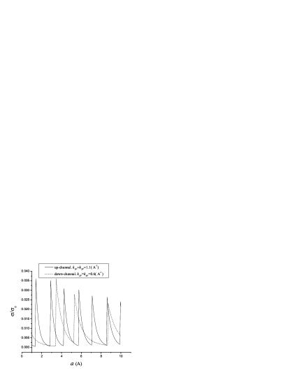
Figure 2: The up and down spin channels conductances for parallel alignment of magnetizations as a function of the middle ferromagnetic layers thickness in the units $\frac{\sigma_{0}}{\mu m^{2}}$ . $k=1$(Å^-1),$q_{0}=0.7$(Å^-1), $b=15$(Å),$c=20$(Å).

Figure 3: The up and down spin channels conductances for antiparallel alignment of magnetizations as a function of the middle ferromagnetic layers thickness in the units $\frac{\sigma_{0}}{\mu m^{2}}$. $k_{1F}=1.1$(Å^-1),$k_{2F}=0.6$(Å^-1) For other parameters see Fig. 2. The relative orientation of outer magnetisations will not affect the value of conductance too much as it dose’t change the position of resonance levels

The most important feature of the obtained expression for the conductance is the pronounced resonances at point, where $Re(B)=0$. These resonances occurs for parallel and anti-parallel orientations of magnetizations of F- layers at different thicknesses of F-layers, so if resonance takes place for example for parallel alignment, it is no resonance for anti-parallel one and so the TMR may have extremely high value. As it is clear from the (Fig. 2,3) conductance as a function of the middle F layers thicknesses for both channels (spin up and down) has sharp maximums and the positions of these maximums are different for parallel and anti-parallel orientation of the magnetizations of F layers.

Figure 4: TMR as a function of the middle layer thickness. $b=15$(Å),$c=20$(Å).

As a result the value of TMR (Fig. 4) reaches extremely high values. However these maximums may be smeared due to the fluctuation of the thickness of the middle layer. We may notice that scattering of electrons in the F layers depends on the electron’s spin and this scattering may give additional contribution to the magnetoresistance. However for thin ferromagnetic layers the resistance of metallic layers is negligible comparing to the tunnel resistance and we may neglect this additional contribution to the magnetoresistance. So to observe the predicted resonances in the case under consideration it is necessary to produce structure with flat enough interfaces.

As it was shown inChshiev[2002] if the thickness of barrier is fluctuating with deviation equal to $3a_{0}$ and the area of this fluctuation constitutes $5\%$ of the total area of the junction the resonance in conductance are completely smeared.

This work was supported by the Russian fund for basic research.

References

(1)
S. A. Wolf, D. D. Awscholom, R .A. Buhrman, J. M. Daughton,
S. von Molnar, M. L. Roukes, A. Y. Chtcheelkanova, and D. M. Treger, Science 294, 488 (2001)
(2)J. S. Moodera, J. Nassar, and G. Mathon,
Annu. Rev. Mater. Sci. 29, 381(1999)
(3) X. Zhang, B. Z.
Li, G. Sun, and F. c. PU, phys. Rev. B 56, 5484(1997)
(4)A. Vedyayev, N. Ryzhanova, R. Vlutters,
and B. Dieny, J. Phys, Condense Matter 10, 5799-808(1998)
(5) F. Montaigne, J, Nassar, A. Vaures, F. Nguyen Van Dau, F, Petroff, A. Schuhl, and A. Fert,
Appl. Phys. Lett. 73, 2829(1998)
(6)M. Chshiev, D. Stoeffler, A. Vedyayev, K. Ounadjela, J. MM. M 240, 146-148(2002)
(7)
D. J.Monsma, J. C. Lodder, Th. A. Popma, and B. Dieny,
Phys. Rev. Lette. 74, 5260(1995)