Macroscopic limit cycle via pure noise-induced phase transition

Abstract

Bistability generated via a pure noise-induced phase transition is reexamined from the view of bifurcations in macroscopic cumulant dynamics. It allows an analytical study of the phase diagram in more general cases than previous methods. In addition using this approach we investigate spatially-extended systems with two degrees of freedom per site. For this system, the analytic solution of the stationary Fokker-Planck equation is not available and a standard mean field approach cannot be used to find noise induced phase transitions. A new approach based on cumulant dynamics predicts a noise-induced phase transition through a Hopf bifurcation leading to a macroscopic limit cycle motion, which is confirmed by numerical simulation.

I INTRODUCTION

The interplay between nonlinear dynamics and noise often generates interesting and counterintuitive phenomena. Popular examples are stochastic resonance Gammaitoni et al. (1998), coherence resonance Anishchenko et al. (2002), and noise induced phase transitions den Broeck et al. (1994, 1997); García-Ojalvo and Sancho (1999). In the latter example noise creates an ordered phase which does not exist in the absence of noise. Unlike noise induced transitions in systems with few degrees of freedom, the noise induced phase transition breaks ergodicity and has the characteristics of a genuine phase transition. In previous studies, many variations of pure noise-induced phase transitions were introduced García-Ojalvo and Sancho (1999). Spatial patterns can be induced via the pure noise-induced phase transition García-Ojalvo et al. (1993); Parrondo et al. (1996); Zaikin and Schimansky-Geier (1998); Buceta et al. (2003). The noise-induced first order phase transition was also shown to be possible Müller et al. (1997); Zaikin et al. (1999); Kim et al. (1998). The systems with colored noise were investigated by various groups García-Ojalvo et al. (1992); Kim et al. (1998); Mangioni et al. (1997, 2000). Furthermore, the bistability created by the noise-induced phase transition exhibits stochastic resonance when a time-periodic perturbation is added Zaikin et al. (2000) and it can lead to propagation of harmonic signals Zaikin et al. (2002). The idea of noise-induced phase transition was also used in coupled Brownain motors. Reimann et al. (1999a, b)

Most of previous investigations take a mean field approach and use the self-consistent condition García-Ojalvo and Sancho (1999); Shiino (1987)

$$\langle x\rangle=\int_{-\infty}^{\infty}xP^{st}\left(x;\langle x\rangle\right)dx.$$ (1)

to determine the mean $\langle x\rangle$ and also bifurcation points. This method yields an exact solution for the phase boundaries. However, to solve Eq. (1) one needs to know the analytic solution of the stationary Fokker-Planck equation $P^{st}\left(x;\langle x\rangle\right)$, which is in general not available. Furthermore, if the system does not have a stationary state (i. e., $\langle x\rangle$ is time-dependent), we must use time-dependent self-consistent condition which is prohibitively more difficult. For certain types of spatially extended stochastic problems, there is an approximate method which replaces stochastic dynamics with effective deterministic dynamics Santos and Sancho (2001). However, the extent of applicability to other models is not known. A general and systematic method is highly desired.

In this paper we present a systematic method to investigate noise-induced phase transitions. While it does not provide exact solutions, the method does not require an analytical expression of the stationary state probability distribution and can be applied to general cases including time-dependent problems. In the following section, we investigate a model system with a single variable introduced by Van den Broeck et al. den Broeck et al. (1994) for which an exact solution is known. The present method predicts a pitchfork bifurcation to an ordered state as the noise intensity increases and also the reentrant transition to a disordered phase at a higher noise intensity. This behavior is qualitatively in a good agreement with the exact results.

Then, we apply the same method to a model with two variables. The model is expected to undergo a noise-induced phase transition to a time-dependent ordered phase for which the time-dependent self-consistent approach is not practical. The present method predicts a Hopf bifurcation to a macroscopic limit cycle phase from a disordered state as the noise intensity increases and shows also a reentrant transition. We also demonstrate that the present method can provide other information such as a period and amplitude of the oscillation.

II NOISE-INDUCED PITCHFORK BIFURCATION

In this section, we consider the following stochastic system of $N$ globally coupled microscopic variables $\{x_{i}\}$:

$$\dot{x_{i}}=f(x_{i})-\frac{D}{N}\sum_{j=1}^{N}(x_{i}-x_{j})+g(x_{i})\xi_{i}(t)$$ (2)

where $D$ is a coupling strength and $\xi_{i}(t)$ is a Gaussian white noise, defined by

$$\langle\xi_{i}(t)\rangle=0,\qquad\langle\xi_{i}(t)\xi_{j}(t^{\prime})\rangle=\sigma^{2}\delta_{ij}\delta(t-t^{\prime}).$$ (3)

Equation (2) is interpreted in the Stratonovich sense.

With certain nonlinear functions $f(x)$ and $g(x)$, Eq. (2) exhibits a phase transition from a disordered phase ($\langle x\rangle=0$) to an ordered phase ($\langle x\rangle\neq 0$) as the noise intensity $\sigma^{2}$ increases. At larger noise intensities the system undergoes a reentrant transition to another disordered phase ($\langle x\rangle=0$) den Broeck et al. (1994, 1997). Since the ordered phase does not exist in the absence of noise, the phenomena is called pure noise-induced phase transition. Van den Broeck et al. den Broeck et al. (1994) originally investigated it using the following nonlinear functions:

$$f(x)=-x(1+x^{2})^{2},\qquad g(x)=1+x^{2}$$ (4)

because a stationary state solution to the corresponding Fokker-Planck equation can be obtained analytically, which allowed them to find the exact phase boundary with the self-consistent equation (1).

In the following, we present a method which allows us to investigate more general cases approximately but without an analytical probability distribution. We apply the method to this model (4) and compare the results with the exact solution and also with numerical simulations.

II.1 Moment Dynamics

Assuming $N\rightarrow\infty$, we write Eq. (2) in a mean field form:

$$\dot{x}=f(x)-D(x-\langle x\rangle)+g(x)\xi(t).$$ (5)

Taking the mean of Eq. (5) under the Stratonovich interpretation, the dynamics of $\langle x\rangle$ is given by

$$\dot{\langle x\rangle}=\langle f(x)\rangle+\frac{\sigma^{2}}{2}\langle g^{\prime}(x)g(x)\rangle.$$ (6)

Expanding $f(x)$ and $g(x)$ in Taylor’s series around $\langle x\rangle$, Eq. (6) forms an infinite set of simultaneous ordinary differential equations:

$$\dot{\langle x\rangle}=\sum_{n=0}\frac{\mu_{n}}{n!}\left\{f^{(n)}(\langle x\rangle)+\frac{\sigma^{2}}{2}[g^{\prime}(\langle x\rangle)g(\langle x\rangle)]^{(n)}\right\}$$ (7)

$$\dot{\mu}_{n} = -Dn\mu_{n}$$ (8)

$$+ \sum_{m=0}\frac{n\mu_{n+m-1}}{m!}\left\{f^{(m)}(\langle x\rangle)+\frac{\sigma^{2}}{2}[g^{\prime}(\langle x\rangle)g(\langle x\rangle)]^{(m)}\right\}$$

$$+ \sum_{m=0}\frac{n(n-1)\mu_{n+m-2}}{m!}\frac{\sigma^{2}}{2}[g^{2}(\langle x\rangle)]^{(m)}.$$

Here, $f^{(n)}$ is the $n$-th order derivative and $\mu_{n}=\langle(x-\langle x\rangle)^{n}\rangle$ the $n$-th central moment with, by definition, $\mu_{0}=1$ and $\mu_{1}=0$.

Some previous studies den Broeck et al. (1997); Garcia-Ojalvo et al. (2002) have considered only the 0-th order term, thereby neglecting the fluctuations $x-\langle x\rangle$, and worked with the equation

$$\langle\dot{x}\rangle=f(\langle x\rangle)+\frac{\sigma^{2}}{2}g^{\prime}(\langle x\rangle)g(\langle x\rangle).$$ (9)

Since this equation does not depend on the coupling constant $D$, it cannot explain the reentrant transition. In fact, Eq. (9) is exact when $D\rightarrow\infty$ under which condition no reentrant transition takes place. den Broeck et al. (1994, 1997) For a finite $D$, one must consider higher order terms.

In order to see how the higher order terms create the reentrant transition, we investigate the previous model Eq. (4). Here we show the equations of motion only for $\langle x\rangle$ and $\mu_{2}$:

$$\langle\dot{x}\rangle = (\sigma^{2}-2)\mu_{3}-\mu_{5}$$ (10)

$$+ \left[\sigma^{2}-1+3(\sigma^{2}-2)\mu_{2}-5\mu_{4}\right]\langle x\rangle$$

$$- 10\mu_{3}\langle x\rangle^{2}+(\sigma^{2}-2-10\mu_{2})\langle x\rangle^{3}-\langle x\rangle^{5}$$

$$\dot{\mu_{2}} = \sigma^{2}+2[2\sigma^{2}-(1+D)]\mu_{2}+\left(3\sigma^{2}-4\right)\mu_{4}-2\mu_{6}$$ (11)

$$+ \left[2(5\sigma^{2}-6)\mu_{3}-10\mu_{5}\right]\langle x\rangle$$

$$+ \left[2\sigma^{2}+12(\sigma^{2}-1)\mu_{2}-20\mu_{4}\right]\langle x\rangle^{2}$$

$$- 20\mu_{3}\langle x\rangle^{3}+(\sigma^{2}-10\mu_{2})\langle x\rangle^{4}.$$

Even with higher order terms, Eq. (10) still does not explicitly depend on the coupling constant. The effect of coupling arises from the dynamics of the second and higher order moments as Eq. (11) indicates.

Noting $f(-x)=-f(x)$ and $g(-x)=g(x)$, the system (5) is invariant under the variable transformation $x\rightarrow-x$. Due to this symmetry the odd moments must be zero when $\langle x\rangle=0$. Then, we find a fixed point at $\langle x\rangle^{*}=0$ and $\mu^{*}_{2n+1}=0$. The even moments at this fixed point are not zero and must be determined by setting the r.h.s. of Eq. (8) to zero. For example, Eq. (11) provides the following equation:

$$\sigma^{2}+2[2\sigma^{2}-(1+D)]\mu^{*}_{2}+\left(3\sigma^{2}-4\right)\mu^{*}_{4}-2\mu^{*}_{6}.=0$$ (12)

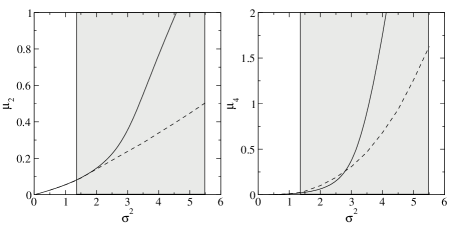
Figure 1: Stationary moments $\mu^{*}_{2}$ (left panel) and $\mu^{*}_{4}$ (right panel) obtained by Gaussian approximation (solid lines) and numerical simulation (dashed lines). The coupling strength $D=10$ is used. The Gaussian approximation appears in a good agreement with the simulation below $\sigma^{2}=2$. However, it overestimates both 2nd and 4th order moments above $\sigma^{2}=2$. This rapid growth causes reentrant transition at a smaller noise intensity than the exact solution. The grey region shows the location of the ordered phase.

A linear stability analysis of Eq. (10) yields the bifurcation condition for a pitchfork bifurcation:

$$\sigma_{c}^{2}-1+3(\sigma_{c}^{2}-2)\mu^{*}_{2}-5\mu^{*}_{4}=0$$ (13)

where $\sigma_{c}$ is a critical noise intensity. Even without the exact knowledge of the higher moments useful information can be derived from Eq. (13). Since both $\mu_{2}$ and $\mu_{4}$ are non-negative, l.h.s. is alway negative for $\sigma^{2}<1$. In this regime the fixed point $\langle x\rangle^{*}=0$ is stable regardless of the magnitude of $D$. For $1<\sigma^{2}<2$, only the 0-th moment term is positive but the other terms are negative and support stability. The bifurcation is possible in this range of noise intensity only when the moments are sufficiently small. Since increasing the coupling strength reduces fluctuation, the bifurcation takes place above a certain magnitude of $D$.

Interestingly, the role of the second moment term changes at $\sigma^{2}=2$. At higher values it supports instability of the fixed point. The 4-th moment term is always negative and supports stability. When $\mu_{4}$ grows faster than $\mu_{2}$ with increasing $\sigma^{2}$, it eventually dominates and l.h.s. of Eq. (13) becomes negative again. Then, the system reenters the disordered phase. In order to determine the critical noise intensity $\sigma_{c}$ from Eq. (13), one needs to know stationary even moments $\mu^{*}_{2}$ and $\mu^{*}_{4}$, which are to be determined by Eq. (12). In turn, it requires $\mu^{*}_{6}$. At the end, all even moments must be simultaneously solved, which is practically impossible for general cases. An approximation is necessary.

II.2 Gaussian Approximation

Figure 2: The phase diagram. The ordered phase ($\langle x\rangle\neq 0$) is above the lines and the disordered phase ($\langle x\rangle=0$) below them. The dashed line is the exact solution obtained by Eq. 1, the solid line is the Gaussian approximation.

When $f(x)$ or $g(x)$ is nonlinear, the stochastic dynamics (2) is not a Gaussian process and in general we cannot solve the system of equations (7) and (8) exactly. For an approximate solution it is convenient to assume a probability distribution $P(x;\langle x\rangle)$ for which the cumulants above a certain order are negligible. We chose here the simplest example where the cumulants above the second order are set to zero (Gaussian approximation). In general, this approximation is quantitatively not justified but reproduces the main features of the noise-induced phase transition, especially the reentrant transition into the disordered phase.

In the Gaussian approximation all odd moments vanish. The even moments can be expressed by the 2nd moment $\mu_{2}$. For example,

$$\mu_{4}=3\mu_{2}^{2}\quad\text{and}\quad\mu_{6}=15\mu_{2}^{3}.$$ (14)

Applying these relations, Eq. (12) becomes

$$\sigma^{2}+2[2\sigma^{2}-(1+D)]\mu_{2}+3\left(3\sigma^{2}-4\right)(\mu^{*}_{2})^{2}-30(\mu^{*}_{2})^{3}=0$$ (15)

which determines $\mu^{*}_{2}$ as a function of $\sigma^{2}$. In turn, we can determine higher order even moments via the Gaussian approximation. Figure 1 plots $\mu^{*}_{2}$ and $\mu^{*}_{4}$ obtained by the Gaussian approximation and also the results of numerical simulation for comparison. Up to $\sigma^{2}=2$, the Gaussian approximation is in a good agreement with the simulation. At higher noise intensities, non-Gaussian behavior becomes large and the Gaussian approximation significantly overestimates the fluctuation.

Once we find all stationary moments, we can quantitatively evaluate the stability condition (13) for $\langle x\rangle$. With the Gaussian approximation (14), the bifurcation condition (13) becomes:

$$\sigma_{c}^{2}-1+3(\sigma_{c}^{2}-2)\mu^{*}_{2}-15(\mu^{*}_{2})^{2}=0\quad$$ (16)

Here, $\mu^{*}_{2}$ must also satisfy Eq. (15) with noise intensity $\sigma_{c}$. In other words, Eqs. (15) and (16) must be solved simultaneously for $\sigma_{c}$ and $\mu_{2}^{*}$.

Figure 2 shows the results and compares them with the exact solution obtained from Eq. (1). Although there is a clear quantitative discrepancy between the approximation and the exact solution the main features, namely the entrant transition into the ordered phase at medium noise intensities and the reentrant into the disordered phase at high intensities is reproduced. As in the exact solution a certain minimum coupling strength is required for the transition to take place.

We can also evaluate the mean $\langle x\rangle$ as a function of $\sigma^{2}$ from Eqs. (10), (14), and (15). The result is plotted in Fig. 3 along with the results of simulation. The agreement near the first transition point is quite good. However, the Gaussian approximation predicts the reentrant transition much earlier than the simulation as mentioned earlier.

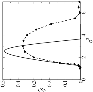
Figure 3: The mean $\langle x\rangle$ by the Gaussian approximation (solid line) and by numerical simulation (dashed line). The coupling strength $D$=10 is used.

We noticed that the present results resemble the phase boundary for the 2-dimensional system with a local coupling examined in Ref. den Broeck et al. (1997) surprisingly well. This coincidence is partly due to the fact that the locally coupled system has much larger fluctuation than the globally coupled system, which induces the reentrant transition at a smaller noise intensity. Since the Gaussian approximation overestimates the fluctuation, it shares some similarity with locally coupled systems.

III Noise-Induced Limit Cycle

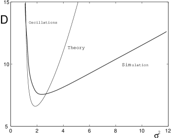
Figure 4: Phase diagram for the two variable case. In the region above the lines we observe oscillations of the mean, below it we do not. The line labeled theory is the analytic solution in the Gaussian approximation, the line labeled simulation is the numerically obtained result for the Langevin dynamics of Eq. 17 and 18 for $N=625$ systems.

In this section we investigate a model with two variables at each site. Multivariate stochastic systems are mathematically quite difficult. Even if the system has a stationary state, it is usually hard to find an analytical expression of its probability distribution. It will be even more difficult if the system does not have a stationary state and the probability distribution is explicitly time-dependent. The lack of an analytical expression of the probability distribution makes the standard method based on the self-consistent equation (1) futile. Direct numerical simulation of multivariate Langevin equations demands more computational power than the single variable cases. However, we expect that the Gaussian approximation provides a degree of accuracy similar to that in the single variable case without increasing mathematical difficulty.

We use the following simple model that keeps a close connection to the previous model:

$$\dot{x_{i}} = f(x_{i})-\frac{D}{N}\sum_{j}(x_{i}-x_{j})+g(x_{i})\xi_{i}(t)-y_{i}$$ (17)

$$\dot{y_{i}} = kx_{i}$$ (18)

with $f(x)$ and $g(x)$ defined by Eq. (4) as before. Again, we expand the dynamical equations in terms of the central moments:

$$\langle\dot{x}\rangle = \sum_{n=0}\frac{\mu_{n,0}}{n!}\left\{f^{(n)}(\langle x\rangle)+\frac{\sigma^{2}}{2}[g^{\prime}(\langle x\rangle)g(\langle x\rangle)]^{(n)}\right\}$$ (19)

$$- \langle y\rangle$$

$$\langle\dot{y}\rangle=k\langle x\rangle$$ (20)

$$\dot{\mu}_{n,m} = -nD\mu_{n,m}-n\mu_{n-1,m+1}$$ (21)

$$+ mk\mu_{n+1,m-1}+mk\mu_{n,m-1}\langle x\rangle-n\mu_{n-1,m}\langle y\rangle$$

$$+ \sum_{\ell=0}\frac{n\mu_{n+\ell-1,m}}{\ell!}\left\{f^{(\ell)}(\langle x\rangle)+\frac{\sigma^{2}}{2}[g^{\prime}(\langle x\rangle)g(\langle x\rangle)]^{(\ell)}\right\}$$

$$+ \sum_{\ell=0}\frac{n(n-1)\mu_{n+\ell-2,m}}{\ell!}\frac{\sigma^{2}}{2}[g^{2}(\langle x\rangle)]^{(\ell)}$$

where $n+m\geq 2$ and $\mu_{n,m}=\left\langle(x-<x>)^{n}(y-<y>)^{m}\right\rangle$ with $\mu_{0,0}=1$ and $\mu_{1,0}=\mu_{0,1}=0$.

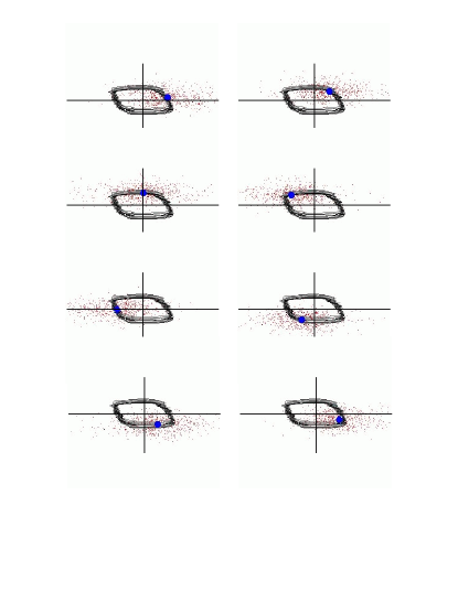
Figure 5: Snapshots of an ensemble of 625 elements in phase-space. The single dots denote the individual elements. The solid circle shows the mean and the line depicts the trajectory of the mean. The time series goes from left to right and from the top to the bottom. Parameter values $D=10$ and $k=0.1$ are used.

For the present model (4), Eqs. (19) and (21) are explicitly written as

$$\langle\dot{x}\rangle = (\sigma^{2}-2)\mu_{3,0}-\mu_{5,0}$$ (22)

$$+ \left[\sigma^{2}-1+3(\sigma^{2}-2)\mu_{2,0}-5\mu_{4,0}\right]\langle x\rangle$$

$$- 10\mu_{3,0}\langle x\rangle^{2}+(\sigma^{2}-2-10\mu_{2,0})\langle x\rangle^{3}$$

$$- \langle x\rangle^{5}-\langle y\rangle$$

$$\dot{\mu}_{2,0} = \sigma^{2}+2\left[2\sigma^{2}-(1+D)\right]\mu_{2,0}$$ (23)

$$- 2\mu_{1,1}+(3\sigma^{2}-4)\mu_{4,0}$$

$$- 2\mu_{6,0}+2\left[(5\sigma^{2}-6)\mu_{3,0}-5\mu_{5,0}\right]\langle x\rangle$$

$$+ 2\left[\sigma^{2}+6(\sigma^{2}-1)\mu_{2,0}-10\mu_{4,0}\right]\langle x\rangle^{2}$$

$$- 20\mu_{3,0}\langle x\rangle^{3}+(\sigma^{2}-10\mu_{2})\langle x\rangle^{4}$$

$$\dot{\mu}_{0,2} = 2k\mu_{1,1}$$ (24)

$$\dot{\mu}_{1,1} = (\sigma^{2}-D-1)\mu_{1,1}+k\mu_{2,0}-\mu_{0,2}+(\sigma^{2}-2)\mu_{3,1}$$ (25)

$$- \mu_{5,1}+\left[3(\sigma^{2}-2)\mu_{2,1}-5\mu_{4,1}\right]\langle x\rangle$$

$$+ \left[3(\sigma^{2}-2)\mu_{1,1}-10\mu_{3,1}\right]\langle x\rangle^{2}$$

$$- 10\mu_{2,1}\langle x\rangle^{3}-5\mu_{1,1}\langle x\rangle^{4}.$$

Here only the lowest order moments are shown.

Taking into account the symmetry of the model, there is at least one fixed point at $\langle x\rangle^{*}=\langle y\rangle^{*}=0$ and $\mu^{*}_{n,2m+1}=\mu^{*}_{2m+1,n}=0$. Stationary even moments are determined by an infinite set of simultaneous equation. Here we show three conditions derived from Eqs. (23)- (25):

$$\sigma^{2}+2\left[2\sigma^{2}-(1+D)\right]\mu^{*}_{2,0}+(3\sigma^{2}-4)\mu^{*}_{4,0}-2\mu^{*}_{6,0}=0,$$ (26)

$$k\mu^{*}_{2,0}-\mu^{*}_{0,2}+\left(\sigma^{2}-2\right)\mu^{*}_{3,1}-\mu^{*}_{5,1}=0$$ (27)

and $\mu^{*}_{1,1}=0$.

Now, we apply the Gaussian approximation to this system. For any two variable Gaussian system, all odd moments are zero ($\mu_{m,n}=0$ for $m+n=\text{odd integer}$) and any even oder moment can be expressed as a product of the 2nd order moments, $\mu_{2,0}$, $\mu_{0,2}$, and $\mu_{1,1}$. For the present model we need only the following relations:

$$\mu_{3,1}=3\mu_{2,0}\mu_{1,1},\quad\mu_{4,0}=3\mu^{2}_{2,0}$$

$$\mu_{5,1}=15\mu^{2}_{2,0}\mu_{1,1},\quad\mu_{6,0}=15\mu^{3}_{2,0}.$$ (28)

Under the Gaussian approximation, the stationary even moments $\mu^{*}_{2,0}$ and $\mu^{*}_{0,2}$ can be determined by Eqs. (26) and (27).

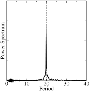
Figure 6: Power spectrum of a limit cycle motion obtained by numerical simulation (solid line) and the period obtained from the linear stability analysis (dashed line). Parameter values are $D$=10, $\sigma^{2}$=2, and $k$=0.1. The agreement is perfect.

The equations of motion (22)-(25) become a five-dimensional dynamical system of $\vec{\xi}$=$\begin{pmatrix}\langle x\rangle&\langle y\rangle&\mu_{2,0}&\mu_{0,2}&\mu_{1,1}\end{pmatrix}$. A standard linear stability analysis yields a Jacobian:

$$\begin{pmatrix}\lambda_{1}&-1&0&0&0\\ k&0&0&0&0\\ 0&0&\lambda_{2}&0&0\\ 0&0&0&0&2k\\ 0&0&k&-1&\lambda_{3}\end{pmatrix}$$ (29)

where

$$\lambda_{1} = \sigma^{2}-1+3(\sigma^{2}-2)\mu^{*}_{2,0}-15(\mu^{*}_{2,0})^{2}$$ (30)

$$\lambda_{2} = 2(2\sigma^{2}-1-D)+6(2\sigma^{2}-4)\mu^{*}_{2,0}-90(\mu^{*}_{2.,0})^{2}$$ (31)

$$\lambda_{3} = \sigma^{2}-1-D+3(\sigma^{2}-2)\mu^{*}_{2,0}-15(\mu^{*}{2,0})^{2}.$$ (32)

The Jacobian (29) is in a block diagonal form and the stability of $\langle x\rangle$ and $\langle y\rangle$ are separated from that of the higher order moments, which makes analytical investigation easier. The 2-by-2 block at the top-left corner determines the stability of $\langle x\rangle^{*}=\langle y\rangle^{*}=0$ and its eigenvalues are given by

$$\lambda=\frac{1}{2}\left(\lambda_{1}\pm\sqrt{\lambda_{1}^{2}-4k}\right),$$ (33)

which indicates that the fixed point becomes unstable at $\lambda_{1}=0$. This bifurcation condition is identical to Eq. (16) and therefore, the two-variable model also undergoes reentrant transition because of the same reason as in the single variable model. Figure 4 compares the phase boundary obtained by the Gaussian approximation and the simulation results. Quantitatively, the disagreement is rather large. However, the qualitative features are correctly captured.

Since the eigenvalue has an imaginary part at the bifurcation point, it is a Hopf bifurcation and a stable Limit cycle is formed above the critical noise intensity, which is confirmed by numerical simulation. Figure 5 shows snapshots of an ensemble of particles. One observes a quite regular limit cycle motion of the mean, even though the system is rather small ($N=625$) and the individual units are spread widely around the mean. The width of the cloud in $x$ direction is much larger than the one in $y$ direction due to small $k$, which is in a good agreement with Eq. (27). Analogous to the single-variable case we will call the oscillating phase the ordered phase and the non-oscillating phase the disordered phase.

From the imaginary part of the eigenvalue the period of oscillation near the bifurcation point is approximately given by $T=2\pi/\sqrt{k}$. Since it does not depend on any moment, this period is valid even without the Gaussian approximation. Indeed it perfectly agrees with numerical simulation as shown in Fig. 6.

If the time evolution of the means is needed, Langevin equation or time-dependent Fokker-Planck equation are usually solved numerically. Numerical simulation of coupled Langevin equations is computationally rather time consuming especially near the bifurcation point due to the finite size effect. One needs a large number of samplings to obtain a reasonable statistics. Furthermore, ensemble averaging is cumbersome since each realization oscillates in a different phase. Numerical integration of time-dependent Fokker-Planck equations does not have a problem of statistical error but often suffers from numerical instability. A special care may be needed. While it is difficult to solve moment dynamics (22), (20) and (23)-(25) analytically even with Gaussian approximation, it is much easier to solve them numerically compared to the Langevin or Fokker-Planck equation. Since the moment dynamics is deterministic, there is no statistical error. The upper panel of Fig. 7 shows the time-evolution of $\langle x\rangle$, $\langle y\rangle$, and $\mu_{2,0}$ with the Gaussian approximation. Other moments, $\mu_{0,2}$ and $\mu_{1,1}$ (not shown) converge to stationary values. The lower panel shows the results of numerical simulation. Only one realization with 10000 particles is shown. Although the amplitude and period are overestimated by the Gaussian approximation, all qualitative features are captured.

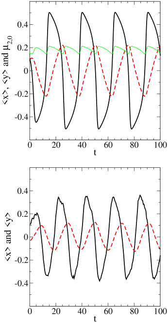
Figure 7: Time evolution of $\langle x\rangle$ (solid line) and $\langle y\rangle$ (dashed line) obtained by numerically solving (20) and (22)-(25) in the Gaussian approximation (upper panel) and Langevin equations (17) and (18) (lower panel). For the Gaussian approximation $\mu_{2,0}$ (thin line) is also shown. Parameters $D=10$, $\sigma^{2}=2$ and $k=0.1$ are used.

Finally, we discuss a special case where $k\ll 1$ (relaxation oscillation limit). In this limit, Eq. (20) indicates $\langle y\rangle$ varies very slowly. Furthermore, from Eq. (27) the fluctuation of the variable $y$ is negligibly small, suggesting that all particles experience the same value of $y$. Since $x$ dynamics is much faster than $y$, a “stationary” probability distribution is formed before $y$ varies. In another word, the variable $y$ in Eq. (19) is just a parameter for the dynamics of $x$. In this case, we can investigate the Hopf bifurcation using the self-consistent equation (1). Following Ref. den Broeck et al. (1994), the stationary distribution is given by

$$P^{st}(x;\langle x\rangle,\langle y\rangle)=\frac{1}{Z}\exp\left[\frac{2}{\sigma^{2}}\int_{0}^{x}dx^{\prime}\left\{-x^{\prime}-\frac{\sigma^{2}}{2}\frac{2x^{\prime}}{1+x^{\prime 2}}-\frac{D(x^{\prime}-\langle x\rangle)+\langle y\rangle}{(1+x^{\prime 2})^{2}}\right\}\right]$$ (34)

where $Z$ is a normalization constant. The self-consistent equation (1) yields a relation between $\langle x\rangle$ and $\langle y\rangle$:

$$\langle x\rangle=\frac{1}{Z}\int_{-\infty}^{+\infty}dx\,\frac{x}{1+x^{2}}\exp\left[-\frac{x^{2}}{\sigma^{2}}+\frac{D}{\sigma^{2}}\frac{1}{1+x^{2}}+\frac{D\langle x\rangle-\langle y\rangle}{\sigma^{2}}\left\{\frac{x}{1+x^{2}}+\arctan x\right\}\right]$$ (35)

which corresponds to a nullcline of the relaxation oscillation. Figure 8 plots the nullcline and an actual trajectory from numerical simulation. The trajectory follows one branch of the nullcline and jumps to the other branch analogous to the deterministic relaxation oscillation. This nullcline is exact. However, its derivation requires an analytical expression of the probability distribution and may not be applicable to other cases. An alternative method such as the Gaussian approximation is useful for general cases where the analytical distribution is not available.

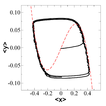
Figure 8: A noise-induced relaxation oscillation. Dashed line: a nullcline determined by Eq. (35). Solid line: a limit cycle trajectory obtained by numerical simulation. Parameter values are $D$=10, $\sigma^{2}$=2, and $k$=0.1. The simulation result follows the theoretical nullcline and jumps to another branch of the nullcline.

IV Conclusions

We have described a general theoretical method useful for the investigation of nonlinear stochastic systems exhibiting noise-induced phase transitions. It is based on the dynamical equations for the central moments. In general the exact solution involves the solution of the infinite dimensional set of ordinary differential equations for these moments. However, even without solving this system useful qualitative information can be gathered from the equations. Furthermore, quantitatively reasonable solutions can be obtained by neglecting the cumulants of the distributions above a certain order and then solving the remaining finite set of equations.

Using this method we investigated two systems. One exhibits a noise induced pitchfork bifurcation, the other one a Hopf bifurcation. In the latter case, the macroscopic quantities oscillate in time when the system is in an ordered phase. This oscillation is purely induced by noise via spontaneous symmetry breaking. The macroscopic oscillation suggests a strong synchronization of microscopic degrees of freedom despite the presence of noise. Actually, it is the noise that generates the macroscopic order. On the other hand a strong noise destroys the order again. The reentrance into the disordered phase is due to the fourth moment, that grows faster with noise intensity than the second moment.

In the Gaussian approximation we have reproduced the basic features of the noise-induced phase transition, namely the existence of a critical coupling strength and the disorder-order-disorder transition.