Properties of Foreshocks and Aftershocks of the Non-Conservative SOC Olami-Feder-Christensen Model: Triggered or Critical Earthquakes?

Abstract

Following Hergarten and Neugebauer StephanPRL who discovered aftershock and foreshock sequences in the Olami-Feder-Christensen (OFC) discrete block-spring earthquake model, we investigate to what degree the simple toppling mechanism of this model is sufficient to account for the properties of earthquake clustering in time and space. Our main finding is that synthetic catalogs generated by the OFC model share practically all properties of real seismicity at a qualitative level, with however significant quantitative differences. We find that OFC catalogs can be in large part described by the concept of triggered seismicity but the properties of foreshocks depend on the mainshock magnitude, in qualitative agreement with the critical earthquake model and in disagreement with simple models of triggered seismicity such as the Epidemic Type Aftershock Sequence (ETAS) model Ogata88 . Many other features of OFC catalogs can be reproduced with the ETAS model with a weaker clustering than real seismicity, i.e. for a very small average number of triggered earthquakes of first generation per mother-earthquake. Our study also evidences the large biases stemming for the constraints used for defining foreshocks and aftershocks.

I Introduction

Describing and modeling the space-time organization of seismicity and understanding the underlying physical mechanisms to quantify the limits of predictability remain important open challenges. Inspired by statistical regularities such as the Gutenberg-Richter GR44 and the Omori Omori laws, a wealth of mechanisms and models have been proposed. New classes of models inspired or derived from statistical physics accompanied and followed the proposition, repeated several times under various forms in the last 25 years, that the space-time organization of seismicity is similar to the behavior of systems made of elements interacting at many scales that exhibit collective behavior such as in critical phase transitions. This led to the concepts of the critical earthquake, of self-organized criticality, and more generally of the seismogenic crust as a self-organized complex system requiring a so-called system approach.

Our purpose here is to study in depth maybe the simplest model of the class of self-organized critical models that exhibit a phenomenology resembling real seismicity, the so-called OFC sandpile model. Real seismicity is usually divided into three major classes of earthquakes, foreshocks, mainshocks, and aftershocks. Many different mechanisms have been discussed to explain these three classes. The OFC model uses only one simple local interaction between discrete fault elements but nevertheless exhibits a sufficiently rich behavior that these three classes of events are observed StephanPRL . The motivation of our present work is thus to study the main characteristics of foreshocks and aftershocks in the OFC model, and to understand the mechanisms responsible for earthquake clustering in the OFC model. For this, we will interpret our analysis of the OFC catalogs in the light of two end-member models representing two opposite views of seismicity. The first one, mentioned above, is the critical earthquake model, which views a mainshock as the special outcome of a global self-organized build-up occurring at smaller scales. The second end-member is called the ETAS (Epidemic-Type Aftershock Sequence) model and is nothing but a phenomenological construction based on the well-documented empirical Gutenberg-Richter law, the Omori law and the aftershock productivity law. In the ETAS model, all earthquakes are put on the same footing, any earthquake can trigger other earthquakes and be triggered by other earthquakes and the distinction between foreshocks, mainshocks and aftershocks is only for convenience and does not reflect any genuine difference. The ETAS model can thus be considered as a realistic statistical null-hypothesis of seismicity.

The plan of our paper is the following. Section II presents the OFC model, section III summarizes the phenomenology of real seismicity, and section IV presents the critical earthquake model and the ETAS model. Section V presents the results obtained for the OFC model, that are compared with real seismicity and with the two reference models (ETAS and critical earthquake models). We discuss in section VI possible mechanisms for foreshocks and aftershocks in the OFC model. Section VII concludes.

II The Olami-Feder-Christensen (OFC) model

The Olami-Feder-Christensen (OFC) model Olami is defined on a discrete system of blocks or of fault elements on a square lattice, each carrying a force. The force $F_{i}$ of a given element $i$ that exceeds a fixed threshold $F_{\rm c}$ (taken equal to $1$ without loss of generality) relaxes to zero. Such a toppling increments the forces on its nearest neighbors by a pulse which is $\alpha\>(\alpha\leq 1/4)$ times the force $F_{i}$ of the unstable element:

$$F_{i}\geq F_{\rm c}\Rightarrow\left\{\begin{array}[]{lll}F_{i}&\rightarrow&0\\ F_{nn}&\rightarrow&F_{nn}+\alpha F_{i}~{}.\end{array}\right.$$ (1)

This loading to nearest-neighbors can in turn destabilize these sites, creating an avalanche. Between events, all $F_{i}$’s increase at the same constant rate, mimicking a uniform tectonic loading. The OFC model can be obtained as a sandpile analogue of block-spring models BurridgeKnopoff , with the interpretation

$$\alpha={1\over n_{i}+k}$$ (2)

where $n_{i}$ is the actual number of neighbors of site $i$. $n_{i}$ is always 4 in the case of a square lattice with rigid-frame boundaries. For free boundary conditions used in this study $n_{i}=4$ in the bulk and $n_{i}=3$ (resp. $2$) at the boundaries (resp. corners). The symbol $k$ denotes the elastic constant of the upper leaf springs, measured relatively to that of the other springs between blocks. The OFC model is conservative for $k=0$ for which $\alpha=0.25$ and is non-conservative for $k>0$ for which $\alpha<0.25$. In the following, we will compare results obtained for $k=0.5,1,2$ and $4$, that is for $\alpha=0.222,0.2,0.167$ and $0.125$.

With open or rigid boundary conditions, this model seems to show self-organized criticality (SOC) Bak ; jensenSOC ; critbook even in the non-conservative case $\alpha<0.25$. SOC is the spontaneous convergence of the dynamics to a statistically stationary state characterized by a time-independent power law distribution of avalanches. The size of an avalanche is taken to be the spanned area $s$. The underlying mechanism for SOC seems to be the invasion of the interior by a region spreading from the boundaries, self-organized by the synchronization or phase-locking forces between the individual elements Others5 .

Long-term correlation between large events have been documented but, only very recently, Ref. StephanPRL found the occurrence of genuine sequences of foreshocks and aftershocks that bear similarities with real earthquake catalogs. This discovery is interesting because it suggests that a unique mechanism is sufficient to produce a Gutenberg-Richter-like distribution as well as realistically looking foreshocks and aftershocks, without the need for viscous crust relaxation or other mechanisms. Similarly, Ref. Huangetla98 found critical precursory activity and aftershock sequences in a sandpile model. However, the precursors and aftershocks resulted from the interplay between the built-in hierarchy of domains and a conservative sandpile dynamics. The remarkable observation of Ref. StephanPRL is that such a hierarchy is not needed for foreshocks and aftershocks to occur, when the sandpile dynamics is dissipative. However, a hierarchy of faults may be needed to obtain a larger number of triggered events than found for the OFC model which is more compatible with real seismicity. Our goal here is to investigate in details the properties of the foreshocks and aftershocks in such a situation, that is, in the OFC model.

Our simulations presented below are performed in two-dimensional square lattices $L\times L$ with $L=512,1024$ and $2048$. Let us give a correspondence between time and space units in the OFC model and in the real seismicity. If we consider that the lattice of $L=1024$ blocks represents a fault of $100\times 100$ km (we neglect the asymmetrical aspect ratio of real faults), which is able to produce an earthquake with magnitude $M=8$, the minimum earthquake of size $s=1$ generated by the OFC model has a length of $\approx 0.1$ km, corresponding to a magnitude 2 earthquake. Ref. StephanPRL documents that the typical waiting time between two events involving at least $1000$ blocks is $10^{-2}$ in the time unit of the model. This event of size $s=1000$ corresponds to a rupture length of $\approx 3$ km or a magnitude $M\approx 5$ earthquake. There are about three events per year with magnitude $M\geq 5$ in Southern California. This gives the correspondence between time units $\rm time_{\rm OFC}$ in the OFC model and in real seismicity:

$${\rm time}_{\rm OFC}=10^{-2}~{}~{}~{}~{}\Longleftrightarrow~{}~{}~{}~{}{\rm time}_{\rm real}=100~{}{\rm days}~{}.$$ (3)

Ref. StephanPRL describe a particularly active aftershock sequence following an event moving $256^{2}$ blocks (magnitude $\approx 7$) lasting ${\rm time}_{\rm OFC}=4\cdot 10^{-6}$ containing about 2500 events. According to (3), this corresponds to an aftershock sequence lasting only one hour. The OFC model clearly does not have the time and space scales right to describe the seismicity in California or in other regions of the world. The number of aftershocks is much smaller in the OFC model than in California, and aftershocks occur at very short times after the mainshock. In the OFC model, aftershocks start at $t_{OFC}=10^{-14}$ after the mainshock (resulting from the numerical precision of the simulation). In real seismicity, aftershocks are only observed after a few minutes following large $M=7$ mainshocks, due to the duration of the mainshock rupture and to the saturation of the seismic network. In real seismicity, aftershocks are also observed over much longer times, from months to years. The aftershock sequences in the OFC model resemble perhaps more those of deep earthquakes, which have few aftershocks Tonga ; omorideep .

III Phenomenology of real seismicity

The empirical properties of real seismicity discussed in this paper are the following.

1. The Gutenberg-Richter (GR) law GR44 states that the density distribution function $P(m)$ of earthquake magnitudes $m$ is

   $$P_{0}(m)dm=b~{}\ln(10)~{}10^{-b(m-m_{d})}~{}dm~{},$$ (4)

   with a $b$-value usually close to $1$. $m_{d}$ is usually a lower bound magnitude of detection, such that $P_{0}(m)$ is normalized to $1$ by summing over all magnitudes above $m_{d}$.

   The qualifying property of SOC in the OFC model is the existence of a GR-like distribution of avalanches sizes. There are several measures of sizes. If we take the size defined as the area $s$ spanned by an avalanche, the distribution of event sizes is exactly given by (4), where the magnitude $m$ is defined by

   $$m=\log_{10}(s)~{}.$$ (5)

   The number of topplings is not exactly equal to $s$ since a site can topple more than once in a given avalanche, possibly being reloaded during its development. However, the difference is negligible for our purpose. No multiple relaxations were observed for $k\geq 2$. For $k=1$, less than 1 multiple relaxation per 100,000 earthquakes was found.

2. The (modified) Omori law Omori ; KK78 ; Utsu describes the decay of the seismicity rate triggered by a mainshock with the time $t$ since the time $t_{c}$ of the mainshock

   $$N_{a}(t)={K_{a}\over(t-t_{c}+c)^{p_{a}}}~{},$$ (6)

   with an Omori exponent $p_{a}$ close to $1$. This decay law can be detected over time scales spanning from weeks up to decades. The time shift constant $c$ ensures a finite seismicity rate just after the mainshock and is often of the order of minutes.

3. The inverse Omori law Papazachos ; KK78 ; JM79 describes the average increase of seismicity observed before a mainshock and is like (6) with $t-t_{c}$ replaced by $t_{c}-t$:

   $$N_{f}(t)={K_{f}\over(t_{c}-t+c)^{p_{f}}}~{},$$ (7)

   with the inverse Omori exponent $p_{f}$ usually close to or slightly smaller than $p_{a}$ Helmfore .

   In contrast with the direct Omori law which can be clearly observed in a single sequence following a mainshock, the inverse Omori law can only be found by stacking many foreshock sequences because there are huge fluctuations of the rate of foreshocks for individual sequences preventing the detection of any acceleration of seismicity. The well-defined acceleration (7) of the seismicity preceding mainshocks emerges only when averaging over many foreshock sequences HSforedata03 .

4. The productivity law documents the growth of the number of triggered aftershocks as a function of the magnitude $m$ of the mainshock:

   $$N_{a}(m)\sim~{}10^{\alpha_{a}m}~{},$$ (8)

   where the exponent $\alpha_{a}$ is usually found in the range $0.7-1$ (see HelmPRL and references therein). This value of the exponent $\alpha_{a}$ may reveal a fractal spatial distribution of aftershocks HelmPRL .

5. Aftershock diffusion. Several studies have reported “aftershock diffusion,” the phenomenon of expansion or migration of aftershock zone with time Tajima1 ; Marsan2 . However, the present state of knowledge on aftershock diffusion is confusing because contradictory results have been obtained, some showing almost systematic diffusion whatever the tectonic setting and in many areas in the world, while others do not find evidences for aftershock diffusion Shaw ; HOS03 . The shift in time from the dominance of the aftershock activity clustered around the mainshock at short times after the mainshock to the delocalized background activity at large times may give rise to an apparent diffusion of the seismicity rate when using standard quantifiers of diffusion processes HOS03 .

6. Foreshock migration. Foreshock migration towards the mainshock as time increases up to the time of the mainshock has also been documented KK78 ; VS81 ; HSforedata03 but may be due to an artifact of the background activity, which dominates the catalog at long times and distances from the mainshock HSforedata03 . Indeed, by an argument symmetrical to that for aftershocks, the shift in time from the dominance of the background activity at large times before the mainshock to that of the foreshock activity clustered around the mainshock at times just before it may be taken as an apparent inverse diffusion of the seismicity rate.

7. The average distance $R_{a}$ between aftershocks and the mainshock rupture epicenter has been found to be proportional to the rupture size of the mainshock, leading to the following scaling law K02

   $$R_{a}\sim 10^{0.5m}\sim s^{0.5}~{},$$ (9)

   relating $R_{a}$ and the mainshock magnitude $m$ or the mainshock rupture surface $s$. A similar law is believed to hold for the average distance $R_{f}$ between foreshocks and the mainshock KBMalinovskaya ; Bowman

8. Foreshock magnitude distribution. Many studies have found that the apparent $b$-value of the magnitude distribution of foreshocks is smaller than that of the magnitude distribution of the background seismicity and of aftershocks (see Helmfore and references therein).

9. Number of foreshocks and aftershocks per mainshock. Foreshocks are less frequent than aftershocks KK76 ; KK78 ; JM79 . The ratio of foreshock to aftershock numbers is in the range 2-4 for $M=5-7$ mainshocks, when selecting foreshocks and aftershocks at a distance in the range $R=50-500$ km from the mainshock and for a time in the range $T=10-100$ days before or after the mainshock KK76 ; KK78 ; JM79 ; VS81 ; Shaw .

IV End-member models of seismicity: ETAS and critical earthquake models

IV.1 The ETAS model

The ETAS (Epidemic-Type Aftershock Sequence) model was introduced in Ogata88 and in KK817 (in a slightly different form). Contrary to what its name may imply, it is not only a model of aftershocks but a general model of seismicity.

This model of multiple cascades of earthquake triggering avoids the division between foreshocks, mainshocks and aftershocks because it uses the same laws to describe all earthquakes. Because of its simplicity, it is natural to consider it as a null hypothesis to explain the OFC catalogs and real data. Its choice as a reference is also natural because it is a nothing but a branching model of earthquake interactions and can thus be considered as a mean field approximation of more complex interaction processes. Branching processes can also be considered as natural mean field approximations of SOC models and in particular of the OFC model Alstrom1 (see also chapter 15 in critbook ). The approximation consists usually in the fact that branching models neglect the loops occurring in the cascade characterizing a given avalanche. Note that standard branching models study the development of a single avalanche while ETAS describe a catalog of earthquakes.

The ETAS model uses three of the above empirical laws as direct inputs (Gutenberg-Richter law (4), Omori’s law (6) and aftershock productivity law (8)). In the ETAS model, a main event of magnitude $m$ triggers its own primary aftershocks (considered as point processes) according to the following distribution in time and space

$$\phi_{m}(r,t)~{}dr~{}dt=K~{}10^{\alpha_{a}m}~{}\frac{\theta~{}c^{\theta}~{}dt}{(t+c)^{1+\theta}}~{}\frac{\mu~{}d^{\mu}~{}dr}{(r+d)^{1+\mu}}~{},$$ (10)

where $r$ is the spatial distance to the main event. The spatial regularization distance $d$ accounts for the finite rupture size. The power law kernel in space with exponent $\mu$ quantifies the fact that the distribution of distances between pairs of events is well described by a power-law KJ1 . The ETAS model assumes that each primary aftershock may trigger its own aftershocks (secondary events) according to the same law, the secondary aftershocks themselves may trigger tertiary aftershocks and so on, creating a cascade process. The exponent $1+\theta$ is not the observable Omori exponent $p_{a}$ but defines the “bare” Omori law for the aftershocks of first generation. The whole series of aftershocks, integrated over the whole space, can be shown to lead to a “renormalized” (or dressed) Omori law, which is the total observable Omori law JGR1Helmsor . To prevent the process from dying out, a small Poisson rate of uncorrelated seismicity driven by plate tectonics is added to represent the effect of the tectonic loading in earthquake nucleation.

The ETAS model predicts the following properties.

1. The same productivity law (8) is found for the total number of events (and not just from the first generation) JGR1Helmsor . This law describes an average power law increase of the number of directly and indirectly triggered earthquakes per triggering earthquake as a function of the mainshock size $s$.

2. The ETAS model finds a global direct Omori law (for aftershocks) different from the “bare” Omori law $\sim 1/(t+c)^{1+\theta}$ defined in (10) for the first generation aftershocks, with a renormalized exponent $p_{a}$ smaller than from $1+\theta$ JGR1Helmsor .

3. An inverse Omori law for foreshocks is found to result simply from the existence of the direct “bare” Omori law (10) and from cascades of multiple triggering Helmfore .

4. The ETAS model predicts a modification of the magnitude distribution (4) before a mainshock of magnitude $m_{M}$, characterized by an increase of the proportion of large earthquakes according to the following expression Helmfore :

   $$P(m|m_{M})=(1-Q(t))P_{0}(m)+Q(t)dP(m)~{},$$ (11)

   where $P_{0}(m)$ is the unconditional GR distribution (4),

   $$dP(m)\sim 10^{-b^{\prime}(m-m_{d})}~{},~{}~{}~{}~{}{\rm with}~{}~{}b^{\prime}=b-\alpha_{a}~{},$$ (12)

   and

   $$Q(t)={C\over(t_{c}-t)^{\nu}}~{},~{}~{}~{}~{}{\rm with}~{}~{}\nu={\theta(b-\alpha_{a})\over\alpha_{a}}~{},$$ (13)

   $t_{c}$ is the time of the mainshock and $C$ is a numerical constant. The prediction (11) with (12,13) is that the magnitude distribution is modified upon the approach of a mainshock by developing a bump in its tail which takes the form of a growing additive power law contribution with a new $b^{\prime}$-value. This prediction has been validated very clearly by numerical simulations of the ETAS model Helmfore .

5. In the ETAS model, the properties of foreshocks are independent of the mainshock magnitude, because the magnitude of each event is not predictable but is given by the GR law with a constant $b$-value Helmfore .

6. By the mechanism of cascades of triggering, the ETAS model also predicts the possibility for large distance and long-time build-up of foreshock activity as well as the migration of foreshocks toward mainshocks. HOS03 ; HSforedata03 .

These predictions of the ETAS model are in good agreement with observations of the seismicity in Southern California HSforedata03 .

IV.2 The critical earthquake model (CEM)

Maybe the first work on accelerated seismicity leading to the concept of criticality is KBMalinovskaya , who observed that the trailing total sum of the source areas of medium size earthquakes accelerates with time on the approach to a large or great earthquake. The theoretical ancestor of the critical earthquake concept can probably be traced back to Verejones , who used a branching model to illustrate a cascade of earthquake ruptures culminating in complete collapse interpreted as a great one. Ref. Allegre82 proposed a renormalization group analysis of a percolation model of damage/rupture prior to an earthquake paralleling Reynolds , which emphasized the critical point nature of earthquake rupture following an inverse cascade from small to large scales. Refs. Voight1 ; Voight2 are probably the first ones to introduce the idea of a time-to-failure analysis in the form of a second order nonlinear differential equation, which for certain values of the parameters leads to a solution of the form of a time-to-failure equation describing the power law acceleration of an observable with time:

$$\epsilon(t)\propto A-B(t_{c}-t)^{z}~{},$$ (14)

where $\epsilon(t)$ is for instance the cumulative Benioff strain (square root of earthquake energy), $A$ and $B$ are positive constants, $t_{c}$ is the critical time of the mainshock and $0<z<1$ is a critical exponent. Ref. Bufe introduced equation (14) to fit and predict large earthquakes. Their justification of (14) was a mechanical model of material damage. Ref. Bufe did not mention the critical earthquake concept. Ref. SS95 proposed to reinterpret Bufe and all these previous works and to generalize them using a statistical physics framework. The concept of a critical earthquake described in Ref. SS95 corresponds to viewing a major or great earthquake as a genuine critical point in the statistical physics sense. In a nutshell, a critical point is characterized by long-range correlations and by power laws describing the behavior of various observables on the approach to the critical point. This concept has been elaborated in subsequent works SS90 ; Huangetla98 ; Bowman ; JS99 ; Ouilrock ; Moraplace ; Zoller1 ; Zoller2 ; Zoller3 ; SS02 . The critical earthquake model predicts a power-law increase of the number, of the cumulative displacement and of the average energy of foreshocks before large earthquakes. According to this model, the modification of seismic activity should be more apparent before larger mainshocks. Therefore, we should measure a positive value for $\alpha_{f}$ characterizing foreshocks. The critical model also predicts that the preparation zone or foreshocks cluster size $R_{f}$ should increase with the mainshock size $s$ as $R_{f}\sim s^{q_{f}}$ with $q_{f}>0$, as observed by Bowman ; KBMalinovskaya (see JS99 for an extended compilation and discussion).

V Properties of the synthetic seismicity generated by the OFC model

V.1 Definitions of foreshocks and aftershocks

The first striking observation, extending the discovery of StephanPRL , is that all the properties of real seismicity discussed in section III are found to exist at least at a qualitative level in synthetic catalogs generated by the OFC model, as we now show.

Deciding what is a foreshock or an aftershock is not straightforward, and several methods have been proposed to define aftershocks or foreshocks Molchan92 ; HOS03 . A clear identification of foreshocks, aftershocks and mainshocks is hindered by the fact that nothing distinguishes them in their seismic signatures: at the present level of resolution of seismic inversions, they are found to have the same double-couple structure and the same radiation patterns Houghjones . It is thus important to consider several alternative definitions.

$\bullet$ Definition $d=0$. The common definition of foreshocks and aftershocks is as follows. A mainshock is first defined as the largest event in a sequence. Foreshocks and aftershocks are then defined as earthquakes in a pre-specified space-time domain around the mainshock, and are thus constrained to be smaller than the mainshock. The space-time window used for foreshock and aftershock selection is defined such that the seismicity rate is much larger than the background seismicity. For simplicity, we choose a space window that covers the whole lattice, and we choose a time window with a duration equal to 1% of the recurrence time of the mainshock, so that the seismicity within this window is much larger than the background seismicity.

However, recent empirical and theoretical studies suggest that this definition might be arbitrary and physically artificial KK817 ; Shaw ; Jones95 ; Houghjones ; Felzer ; HelmPRL ; HSforedata03 . Indeed, the magnitude of an earthquake seems to be unpredictable HelmPRL , therefore the same mechanisms responsible for the triggering of small earthquakes (usual “aftershocks” for $d=0$) may also explain the triggering of larger earthquakes (defined as “mainshocks” for $d=0$). This hypothesis has been tested in HSforedata03 and accounts very well for the properties of earthquake clustering in real seismicity. We thus use two other definitions of foreshocks and aftershocks, which do not constrain aftershocks and foreshocks to be smaller than the mainshock, in order to test how the selection procedure impacts on foreshock and aftershock properties.

$\bullet$ Definition $d=1$. Mainshocks are now defined as any earthquake that was not preceded by a larger earthquake within a time window equal to 1% of the mainshock recurrence time, but can be followed by a larger event. This rule aims to select as aftershocks the events that have been triggered directly or indirectly by the mainshock, removing the influence of large earthquakes that occurred before the mainshock. We use the same space-time domain as for $d=0$ to select foreshocks and aftershocks around the mainshock. Foreshocks are thus smaller than mainshocks but aftershocks can be larger.

$\bullet$ Definition $d=2$. Same as $d=1$ without any constraint on the aftershocks and mainshocks: each event of appropriate size is a mainshock, preceded by foreshocks and aftershocks which are selected solely on the basis of their belonging to the pre-specified space-time domain around the mainshock, with arbitrary magnitudes. For foreshocks, this corresponds to the “Type II” foreshocks introduced in Helmfore ; HSforedata03 in order to remove any spurious dependence of foreshock properties on the mainshock magnitude.

For $d=2$, each earthquake can be a foreshock or an aftershock to several mainshocks and can also be a mainshock.

V.2 Direct (aftershocks) and inverse (foreshocks) Omori laws

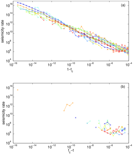
Figure 1: $15$ individual sequences of aftershocks (a) and foreshocks (b), for mainshocks of size $s>2048$ with more than $1000$ foreshocks or aftershocks, generated in a system of size $L=2048$, dissipation index $k=2$ and selected with definition $d=0$.

Figure 1 shows $15$ individual sequences of foreshocks (bottom) and aftershocks (top), for mainshocks of size $s>2048$ with more than $1000$ foreshocks or aftershocks, generated in a system of size $L=2048$, dissipation index $k=2$ and selected with definition $d=0$. The direct Omori law (6) is strikingly clear for each individual sequence while, for foreshocks, there is almost no increase of the seismic rate for individual sequences: the inverse Omori law (7) is only observed when stacking many sequences, like in the ETAS model Helmfore . This is the clearest indication that the foreshock activity may be better described by a cascade ETAS-type model than by a critical earthquake model (but see below for other observations that may modulate this preliminary conclusion). The OFC model shares this property with empirical seismicity HSforedata03 and with the ETAS model Helmfore .

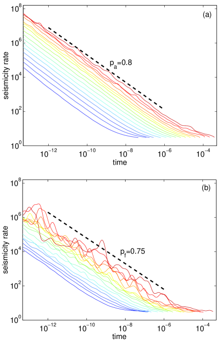
Figure 2: Direct ((a), aftershocks) and inverse ((b), foreshocks) Omori law for synthetic catalogs generated with the OFC model with $L=2048$, dissipation index $k=2$ and definition $d=0$. The seismicity rate is normalized by the background rate and by the number of mainshocks in each class. The mainshock size increases from $s=2$ (bottom curve) to $s=2^{16}$ (top curve) with a factor 2 between each curve.

We now describe the results obtained by averaging over a large number of sequences, which allow us to decrease the noise level and to look at smaller mainshocks. We have generated synthetic catalogs with the OFC model, using a lattice size $L=128,256,512,1024,2048$ and different values of the dissipation index $k=0.5,1,2,4$. For each catalog, we have selected aftershocks and foreshocks following the different definitions $d=0,1,2$ explained in section V.1. We have then stacked all sequences by superposing all sequences translated in time so that the mainshock occurs at time $t=0$. We have first analyzed the change of the seismicity rate before and after a mainshock. For each range of mainshock size $s$ between 2 and $2^{16}$, increasing by a factor 2 between each class, we compute the average seismicity rate $N_{f}(t)$ and $N_{a}(t)$ as a function of the time before and after the mainshock. The results for $L=2048$, $k=2$ and $d=0$ are illustrated in Figure 2. The rate of aftershocks obeys the direct Omori law (6) and the increase of the seismicity rate observed when averaging over many sequences follows the inverse Omori law (7). We measure the Omori exponents $p_{f}$ and $p_{a}$ by fitting the number $N_{a}(t)$ of aftershocks and the number $N_{f}(t)$ of foreshocks by a power law $\sim 1/|t|^{p_{a,f}}$ using a linear regression of $\ln(N)$ as a function of $\ln|t|$, in the time interval $|t|>5\cdot 10^{-14}$ and $|t|<t_{max}$, where the upper bound $t_{max}$ is given by the condition that the seismicity rate is much larger than the background level.

The duration of aftershock or foreshock sequences is much smaller than the average recurrence time of earthquakes. This is also shown in Figure 1 of Ref. StephanPRL , which represents the distribution of inter-event times. A deviation from the Poisson distribution is evident only for small times compared to the average inter-event times.

Table LABEL:tab1 provides the values of the exponents $p_{a}$ and $p_{f}$ as a function of $L$, $k$ and $d$. We find similar Omori exponents for foreshocks and aftershocks with $p_{f}\leq p_{a}<1$. We observe the same time-dependence of the seismicity rate (same exponents $p_{a}$ and $p_{f}$) for all mainshock sizes, only the absolute value of the seismicity rate depends on the mainshock magnitude. The exponents $p_{a}$ and $p_{f}$ are found to increase with $k$ from $p_{a}\approx 0.5$ for $k=0.5$ to $p_{a}\approx 0.9$ for $k=4$, but the duration of the aftershock and foreshock sequence does not change significantly with $k$. The Omori exponents do not depend on the rules of selection $d$. The number of foreshocks and aftershocks thus increases if the dissipation increases, and is almost negligible in the non-dissipative case.

V.3 Dependence of the number of aftershocks and foreshocks with the mainshock size

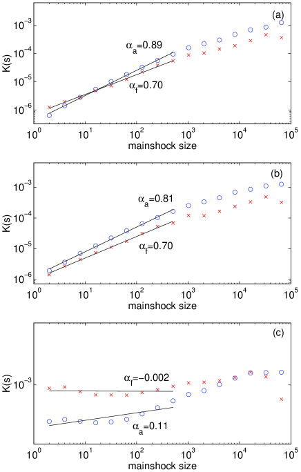
Figure 3: Productivity of aftershocks $K_{a}$ (circles) and foreshocks $K_{f}$ (crosses) as a function of the mainshock size $s$ for synthetic catalogs generated with the OFC model with $L=2048$, dissipation index $k=2$ and definition $d=0$ (a), $d=1$ (b) and $d=2$ (c).

Figure 3 represents the dependence of the number of aftershocks and foreshocks with the mainshock size, for different rules of selection $d=0,1,2$. We observe a power-law increase of the number of foreshocks $K_{f}$ and aftershocks $K_{a}$ defined in (6) and (7) with the mainshock size $s$ according to

$$K_{a}(s)\sim s^{\alpha_{a}}~{},~{}~{}~{}~{}{\rm and}~{}~{}~{}~{}K_{f}(s)\sim s^{\alpha_{f}}~{},$$ (15)

for $s<10^{3}$. The exponents $\alpha_{a}$ and $\alpha_{f}$ measured for $s<1000$ increase with the dissipation index $k$ (see Table 1). The results are very similar for $d=1$ and $d=0$. The exponent $\alpha_{a}$ is slightly smaller for $d=1$ than for $d=0$, because for $d=0$ we impose the aftershocks to be smaller than mainshocks. Small events are more likely to trigger an event larger than themselves than larger mainshocks and thus to be rejected from the analysis. Therefore the rule $d=0$ underestimates the number of earthquakes triggered by small mainshocks.

For $d=2$ and for small $s$, $K_{a}(s)$ and $K_{f}(s)$ are much larger than with $d=0$, and are almost independent of $s$ for $s<100$. This results from the fact that, for $d=2$ a significant fraction of “mainshocks” are triggered by a previous larger event, and thus the events classified as aftershocks may be in fact triggered by earthquakes that occurred before their “mainshock”. The results obtained with $d=2$ recovers those obtained with $d=0$ and $d=1$ for large $s$. The correct value of the exponent $\alpha_{a}$ of the aftershocks productivity law is thus the value obtained for $d=1$.

The number of foreshocks is generally smaller than the number of aftershocks and increases more slowly with $s$ ($\alpha_{f}\leq\alpha_{a}$).

For large mainshock sizes $s>1000$, we observe a saturation of $K_{a}$ and $K_{f}$, and the numbers of foreshocks and aftershocks increase slower with $s$ than predicted by (15). This saturation size does not depend neither on $k$ nor on $L$. The effect of the system size $L$ is only to change the shape of the functional form of $K_{a}(s)$ and $K_{f}(s)$ for large $s$: the saturation of $K_{a,f}(s)$ for $s>1000$ is more obvious for smaller $L$.

V.4 Spatial distribution of foreshocks and aftershocks

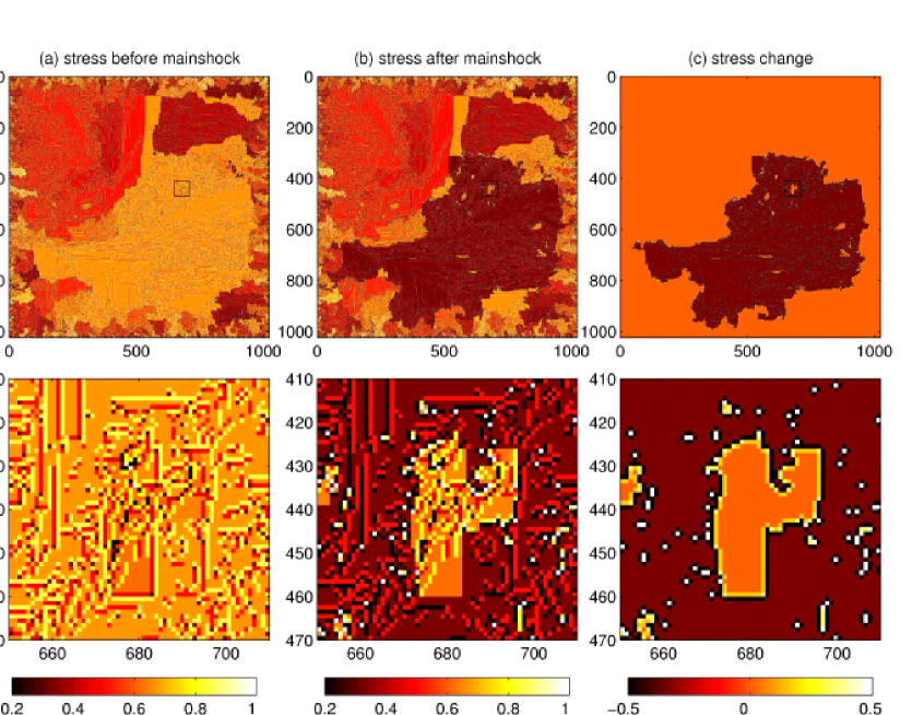
Figure 4: Stress field immediately before (a) and after (b) a mainshock. The stress change due to the mainshock in shown in (c). The elements that broke during the avalanche are shown in dark in (c) (stress decrease), and were mostly close to the rupture threshold before the mainshock (light gray in (a)). The upper panels show the whole grid of size $L=1024$ and the lower plots represent a subset of the grid delineated by the square in the upper plot.

Figure 4 shows the stress field immediately before and after a large mainshock. Following the mainshock, many elements on the boundary of the avalanche and within the avalanche have been loaded by the rupture, and are likely to generate aftershocks after the mainshock. There are a few large patches of elements within the avalanche that did not break during the mainshock, as illustrated in the lower panels of Figure 4, but most aftershocks initiate on smaller clusters of a few unbroken elements shown as white spots in the central lower panel of Figure 4. The density of such white spots observed in this square is typical of the rest of the stress field over the area spanned by the mainshock. In the language of seismicity, such white spots are “asperities” which carry a large stress after the mainshock and are nucleation point for future aftershocks. These white spots are also found on the avalanche boundaries.

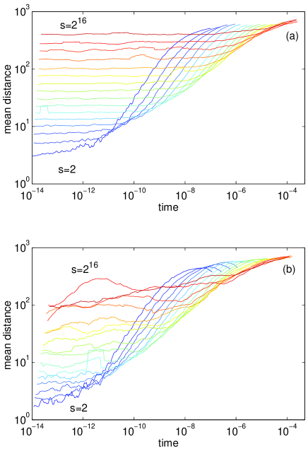
Figure 5: Average distance between mainshocks and aftershocks (a) and mainshocks and foreshocks (b) as a function of the time after (a) or before (b) the mainshock, for synthetic catalogs generated with the OFC model with $L=2048$, dissipation index $k=2$ and definition $d=0$. Each curve corresponds to a different mainshock size size increasing from $s=2$ (bottom curve) to $s=2^{16}$ (top curve) with a factor 2 between each curve.

The aftershock cluster size $R_{a}$, defined as the average distance between the mainshock and its aftershocks, is close to the mainshock size $\ell=\sqrt{s}$ at small times, and then increases to a value close to the system size $L$ at large times (see Figure 5). This crossover of $R_{a}(t)$ corresponds to a transition between the aftershock activity at small times and short distances from (or within the area spanned by) the mainshock, to the uncorrelated seismicity at larger times after the mainshock and with a uniform spatial distribution. We observe the same pattern for the spatial distribution of foreshocks. The time of the crossover of $R_{a}(t)$ and $R_{f}(t)$ increases with $s$ because the number of foreshocks and aftershocks increases with $s$ and thus remain for a longer time above the uncorrelated background seismicity. In the short times regime where uncorrelated seismicity is negligible, we find a very weak, if any, diffusion of aftershocks, as measured by an increase $R_{a}\sim t^{H_{a}}$ of the aftershock zone size with the time after the mainshock. Similarly, we observe a very weak migration of foreshocks toward the mainshock, characterized by a decrease $R_{f}\sim(t_{c}-t)^{H_{f}}$ of the foreshock zone as the mainshock approaches. The Hurst exponents $H_{a}$ and $H_{f}$ are not statistically different from $0$, showing that the size of the foreshock and aftershock zones do not change significantly with time.

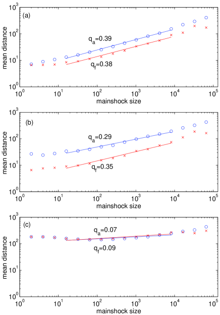
Figure 6: Average distances $R_{a}$ (circles) and $R_{f}$ (crosses) as a function of the mainshock size $s$, for $k=2$, $L=2048$, and for definitions $d=0$ (a), $d=1$ (b) and $d=2$ (c). The continuous lines are fits of $R_{a,f}(s)$ by a power-law $s^{q}$.

We observe on Figure 6 a power-law increase of aftershock zone size and of the foreshock zone size with the mainshock size according to

$$R_{a}(s)\sim s^{q_{a}}~{},~{}~{}~{}~{}{\rm and}~{}~{}~{}~{}R_{f}(s)\sim s^{q_{f}}~{},$$ (16)

in the range $10<s<10^{4}$. The exponents $q_{a}$ and $q_{f}$ are given in Table 1 as a function of $k$, $L$, and $d$. In contrast with real seismicity, the aftershock zone area is not proportional to the mainshock size $s^{0.5}$, but it increases slower with $s$ ($q_{a}\approx 0.3<0.5$ for $d=0$ or 1). This is probably due to the effect of secondary aftershocks, which increase the effective size of the aftershock zone for small mainshocks. Secondary aftershocks are more important for $d=1$ than for $d=0$, which explains why $q_{a}$ is smaller for $d=1$ than for $d=0$. The average value of the foreshock zone (“zone of mainshock preparation”) is smaller than the aftershock zone, except for definition $d=2$.

An increase of $R_{f}$ with $s$ according to (16) has been reported by Ref. KBMalinovskaya ; Bowman for individual sequences, with an exponent $q_{f}=0.44$ Bowman , but was not observed by Ref. HSforedata03 when using stacked sequences and when allowing foreshocks to be larger that the mainshock ($d=2$). This increase of $R_{f}$ with $s$ is not observed by the ETAS model, because the magnitude of each earthquake is drawn at random, independently of previous seismicity, and thus all properties of foreshocks must be independent of the mainshock size.

For $d=2$, the average zone sizes $R_{a}$ and of $R_{f}$ are much larger than for $d=0$, because we include foreshocks and aftershocks larger than the mainshock. ¿For $s<1000$, the values of $R_{a}$ and $R_{f}$ are almost constant of the order of $R_{a,f}\approx 100$. This may reflect the fact that, for $d=2$ and for small mainshocks, most aftershocks are not triggered by the mainshock but by a previous larger event.

V.5 Distribution of avalanche sizes

For the whole catalogs, the distribution of event sizes is a power-law characterized by an exponent $b$, with an exponential roll-off for large sizes $s>10^{-3}L^{2}$. Table LABEL:tab1 shows that the exponent $b$ increases as the dissipation index increases, from $b\approx 0.7$ for $k=0.5$ to the realistic value $b\approx 0.95$ for $k=4$, in agreement with previous works Lise ; Grassberger .

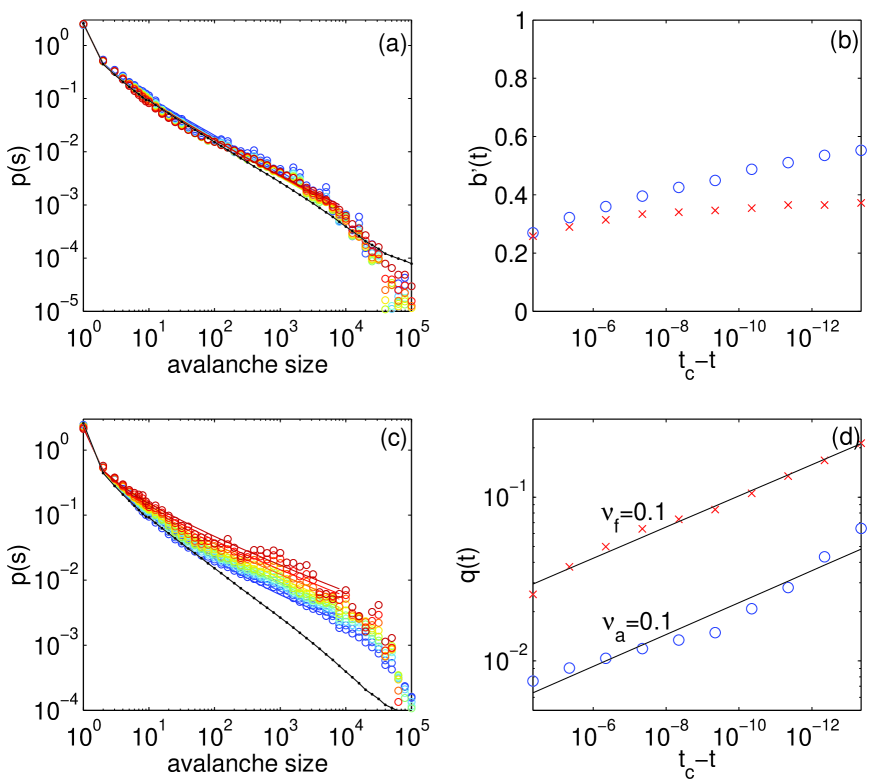
Figure 7: Aftershock (a) and foreshock (c) size distribution as a function of the time before or after the mainshock, for $k=2$ and $L=2048$, and for a mainshock size in the range $s=2048-4096$. Aftershocks were selected with $d=1$ and foreshocks with $d=2$ (without constrains on the magnitude of foreshocks and aftershocks). The avalanche size distributions are constructed with a logarithmic binning (linear bin in magnitudes), whose slope gives the GR $b$-value. The black line in (a) in (c) shows the size distribution for the whole catalog for reference. The different colors from blue to red correspond to different time windows closer and closer to the mainshock, from $|t_{c}-t|=5\times 10^{-5}$ to $|t_{c}-t|=5\times 10^{-14}$. The colored lines in (a) and (c) are the fit of the foreshock and aftershock magnitude distribution $P(m)$ (with $m=\log_{10}(s)$ as defined in (5)) by expression (11). The corresponding values of $b^{\prime}(t)$ (12) and $Q(t)$ (13) are shown in (b) and (d) for foreshocks (crosses) and aftershocks (circles), as a function of time before/after the mainshock.

Figures 7 test the stationarity of the magnitude distribution for foreshocks and aftershocks. The magnitude distributions for foreshocks and aftershocks have been fitted with expression (11) and these fits are shown as the colored lines. The deviation of the magnitude distribution from the average GR law for foreshocks and aftershocks are well represented by (11) with $b^{\prime}$ in the range $0.3-0.5$ and with $Q(t)$ increasing as a power law according to (13) with $\nu\approx 0.1$ for foreshocks and for aftershocks.

For aftershocks, the time-dependence of $Q(t)$ describes a decrease of the deviation from the GR law for latter aftershocks. While these fits are good, there is an important caveat: the prediction $b^{\prime}=b-\alpha$ of the ETAS model is not valid here, as the OFC model gives $\alpha_{a}\approx 0.8$ for $k=2$, which is slightly larger than $b=0.78$. This regime $\alpha_{a}>b$ gives an explosive behavior in the ETAS model with a stochastic finite time singularity Sorhelm02 unless the GR law is truncated by an upper bound or is rolling over to a faster decay for the large earthquake sizes.

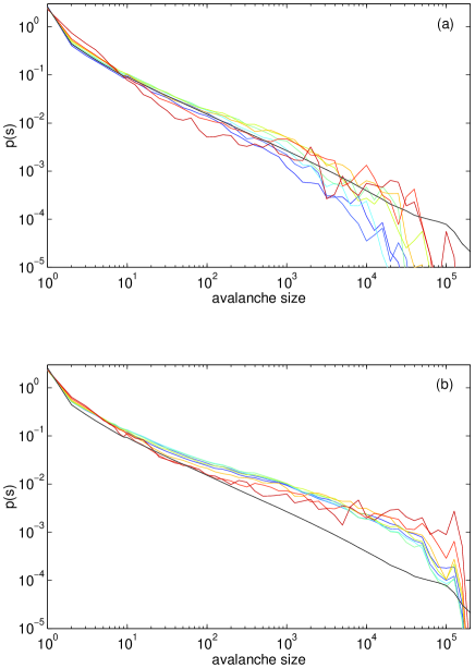
Figure 8: Aftershock (a) and foreshock (b) size distribution for $k=2$ and $L=2048$. Aftershocks ($d=1$) and foreshocks ($d=2$) are selected in a time window $5\times 10^{-11}<|t_{c}-t|<5\times 10^{-10}$. Each curve corresponds to a different mainshock size between $s=4$ (blue curve) and $s=2^{16}$ (red curve) increasing by a factor 4 between each curve. The black line shows the (unconditional) distribution of the whole catalog.

The modification of the magnitude distribution for aftershocks in the OFC model, is much weaker than for foreshocks, but is significant. This implies that the magnitude distribution in the OFC model is not stationary because the magnitude of triggered earthquakes is correlated with the mainshock magnitude, in contradiction with a crucial hypothesis of the ETAS model and with real catalogs. Figure 8 shows that, for $d=1$ (no constraint on aftershock magnitudes), the change of the magnitude distribution is almost independent on the mainshock magnitude (like in the ETAS model). However, there is a larger proportion of medium-size events for smaller mainshocks than for larger ones. This means that smaller mainshocks have a tendency to trigger smaller aftershocks than larger mainshocks.

This result is in contradiction with the ETAS model, which does not reproduce a dependence of the aftershock magnitude as a function of the size of the triggering earthquake or as a function of the time since the mainshock. Observations of real seismicity HelmPRL do not show any dependence between the aftershock magnitude and the mainshock magnitude, but the catalogs available are much smaller than for our OFC simulations.

VI Mechanisms for foreshocks and aftershocks in the OFC model

Is the increase of the number of aftershocks and foreshocks with the mainshock magnitude real or is it just the result of a selection bias introduced by the standard definition $d=0$, which requires that mainshocks are the largest events in the cluster? Indeed, in the OFC catalogs, the clear power-law increase of the number of aftershocks and foreshocks with the size $s$ of the mainshock, found when we define the mainshock as the largest event ($d=0$), almost disappears when aftershocks or foreshocks are not constrained to be smaller than the mainshock ($d=2$), as shown in Figure 3. The question of the impact of the definition is thus essential.

For foreshocks, we consider two possible interpretations, the ETAS model described in section IV.1 and the critical earthquake model (CEM) summarized in section IV.2. The fact that, using $d=0$, both the number of foreshocks and the average foreshock cluster size increase with the mainshock size $s$ seems to favor the critical model, but Ref. Helmfore have shown that the constraint that foreshocks must be smaller than the mainshock ($d=0$) leads to an artificial increase of the number of foreshocks and of the foreshock cluster size with $s$ (see Fig. 5 of Helmfore ). However, this spurious increase of the number of foreshocks with the mainshock magnitude should be observed only for small $s$, and should not exist in the case $d=2$ (without constraints on foreshock and mainshock magnitudes). The fact that a weak increase of the number of foreshocks with $s$ is observed even for very large $s$ and for all definitions $d=0,1,2$ suggests that the effect is genuine. Such a dependence of foreshock properties on the mainshock size cannot be reproduced with the ETAS model, but suggest that the critical model provides a more relevant description of these observations.

The case $d=2$ destroys the dependence of the aftershock number with $s$ for small $s$, which is a real physical property of aftershocks because it is also observed for $d=1$. The same effect may also be at work for foreshocks and explain why, if the properties of foreshocks are physically dependent on the mainshock magnitude, this dependence is not observed when using $d=2$. Definition $d=2$ may be mixing “critical foreshocks”, i.e. events that belong to the preparation phase of the future mainshock, with “triggering-triggered” pairs (which are the usual “foreshock-mainshock” pairs in the ETAS model). Thus, the absence of conditioning ($d=2$) seems to destroy the dependence of both the foreshock and aftershock properties with the mainshock magnitudes, i.e., $\alpha_{a,f}\approx 0$ and $q_{a,f}\approx 0$ both for foreshocks and aftershocks. But, for aftershocks, we know for a truth that the dependence of the number ($\alpha_{a}$) and the cluster size ($q_{a}$) are real and physical because they are observed in the case $d=1$ which do not constrain aftershocks to be smaller than the mainshocks.

For aftershocks selected according to $d=2$ and for small mainshock sizes $s$, the scenario, according to which most aftershocks are not triggered by the mainshock per se but by a previous larger event, seems to explain both the fact that (i) the number of aftershocks is almost constant with $s$ for $s<100$ and (ii) the size of the aftershock cluster is almost constant with $s$ for small $s$. It is however surprising, if this interpretation is correct, that we observe a pure Omori law for aftershocks and foreshocks in the case $d=2$, without any change in the Omori exponent with $s$ and without any roll-off at small times.

The observations that earthquake clustering in the OFC model is much weaker than for real seismicity implies that the “branching ratio” (average number of triggered earthquakes of first generation per mother-earthquake) must be close to $0$ for the ETAS model to match the OFC model. But such a small branching ratio would lead to Omori’s exponent larger than $1$, in contradiction with our simulations. Thus, the pure branching model of triggered seismicity is insufficient to fully account for the quantitative aspect of the OFC seismicity.

In order to better understand the mechanism responsible for aftershocks in the OFC model, we have imposed several types of perturbations to the normal course of an OFC simulation to obtain the response of the system. First, we have simulated random isolated disturbances consisting in choosing randomly and independently $1024$ sites and adding to them random amounts of stress drawn in the interval $[0,0.01]$ or $[0,0.1]$. Repeating such disturbance 100000 times, we find no observable seismicity triggered by this perturbation. This shows that the aftershocks require a coherent spatial organization over a broad area. In contrast, pasting (or grafting) the stress map as shown in figure 4 of those sites that participated in a given large mainshock in a given simulation and their nearest neighbors onto another independent simulation gives a perfect Omori law following this graft in this second simulation as if the foreign stress map of the first simulation was part of the second simulation. The resulting aftershock sequences are similar to natural sequences. This demonstrates that the presence of asperities close to the failure threshold inside the boundary of the avalanche can produce realistic aftershock sequences with an Omori law temporal decay. To investigate further if it is the spatial connectivity of the perturbation which is important to get aftershocks, we have also raised simultaneously the stress by various amounts within squares of size $64\times 64$. Performing this perturbation 40000 times at random instants, we observe that this sometimes results in quite large earthquakes immediately following the perturbation, but there is no significant activity afterwards, and nothing that looks like an Omori law of aftershocks. Thus, it seems impossible to generate aftershocks by introducing a random or deterministic spatially extended perturbation. This suggests that aftershocks require not only the occurrence of mainshocks to redistribute stress but also a spatial organization of the stress field prior to the mainshock so that many “asperities” (as illustrated in figure 4) can be created by the interplay of the stress organization before the mainshock and the stress redistribution by the mainshock.

VII Conclusion

The results obtained in this paper can be viewed from two different perspectives. On the one hand, we are adding to the phenomenology of one of the most studied model of self-organized criticality. Extending Hergarten and Neugebauer’s announcement StephanPRL , we have shown evidence that the self-organized critical state of the OFC model is much richer than previously thought, with important correlation patterns in space and time between avalanches. We have obtained quantitative scaling laws describing the spatio-temporal clustering of events in the OFC model. On the other hand, we have shown that what is probably the simplest possible mechanism for the generation of earthquakes (slow tectonic loading and sudden stress relaxation with local stress redistribution) is sufficient to recover essentially all known properties documented in seismic catalogs, at a qualitative level. Specifically, we have found that foreshocks and aftershocks follow the inverse and direct Omori power laws, as in real seismicity but with smaller exponents. We have found the productivity power law of aftershocks as in real seismicity. In contrast with real seismicity, we also found a power-law increase of foreshock productivity with the mainshock size. The nucleation of aftershocks at “asperities” located on the mainshock rupture plane or on the boundary of the avalanche is also in agreement with seismic observations. These findings are interesting because they add on the list of possible mechanisms for foreshocks and aftershocks that have been discussed previously in the literature.

We also found that the predictability increases with the mainshock magnitude in the OFC model, because the number of foreshocks seems to increase with the magnitude of the mainshock, a feature that is not observed in real seismicity HSforedata03 . See the debate in Nature at http://helix.nature.com/debates/earthquake/ and PC94 ; Geller for related discussions on the predictability of real earthquakes and the use of models from statistical physics.

While most of the OFC dynamics can be qualitatively captured by the simple ETAS model of triggered seismicity, this property that the number of foreshocks seems to increase with the magnitude of the mainshock is better explained by the critical earthquake model. We have systematically compared the statistical properties of the avalanches generated by the dynamics of the OFC model with those predicted by the ETAS model on the one hand and by the critical earthquake model on the other hand. These two models constitute end-member models of seismicity. We can conclude that, while the detailed quantitative predictions of the ETAS model for its application to the OFC model are not exactly right, the physical mechanism of cascades of triggered events inherent in the ETAS model captures at least qualitatively the observed regularities found in the OFC model. This suggests a picture in which future avalanches are triggered by past avalanches through “asperities” located either within the plane of past avalanches or at their boundaries. In addition, we find that this triggering mechanism presents a degree of cooperativity, as the number of foreshocks increases with the mainshock size. In other words, this suggests that asperities interact via avalanches, and when their number and size increase in a given location, they can produce larger avalanches.

Table 1: Aftershock and foreshock properties in the OFC model as a function of the system size $L$ and of the dissipation index $k$, for different definitions of foreshocks and aftershocks $d$ (see section V.1). $b$ is the exponent of the cumulative distribution of avalanche sizes, measured for the whole catalog and discussed in section V.5. $p_{a}$ and $p_{f}$ are the exponents of the direct and inverse Omori laws (see section V.2). $\alpha_{a}$ and $\alpha_{f}$ characterize the dependence of the aftershock and foreshock rate with the mainshock size $s$ (see section V.3). $q_{a}$ and $q_{f}$ describe the scaling of the aftershocks and foreshock zone size with $s$ (see section V.4). $N_{\rm max}$ is the maximum rate of aftershocks at $t=10^{-14}$ normalized by the background rate.

$k$	$L$	$b$	$d$	$p_{a}$	$p_{f}$	$\alpha_{a}$	$\alpha_{f}$	$q_{a}$	$q_{f}$	$N_{\rm max}$
$0.5$	$512$	$0.71$	$0$	$0.5$	$0.5$	$-0.2$	$-0.3$			$10^{3}$
$0.5$	$512$		$1$	$0.5$	$0.5$	$-0.2$				$10^{3}$
$0.5$	$512$		$2$	$0.5$	$0.5$	$-0.3$	$-0.5$			$10^{3}$
$0.5$	$1024$	$0.67$	$0$	$0.6$	$0.6$	$0.06$	$-0.29$			$10^{3}$
$0.5$	$1024$		$1$	$0.6$	$0.6$	$0.05$	$-0.21$			$10^{3}$
$0.5$	$1024$		$2$	$0.5$	$0.5$	$-0.42$	$-0.21$			$10^{3}$
$1$	$512$	$0.76$	$0$	$0.65$	$0.65$	$0.63$	$0.36$			$10^{6}$
$1$	$512$		$1$	$0.65$	$0.65$	$0.6$	$0.31$			$10^{6}$
$1$	$512$		$2$	$0.65$	$0.65$	$0.11$	$-0.1$			$10^{6}$
$1$	$1024$	$0.73$	$0$	$0.65$	$0.65$	$0.63$	$0.35$	$0.20$	$0.17$	$10^{6}$
$1$	$1024$		$1$	$0.65$	$0.65$	$0.58$	$0.34$	$0.19$	$0.13$	$10^{6}$
$1$	$1024$		$2$	$0.65$	$0.65$	$0.11$	$0.09$	$0.11$	$0.14$	$10^{6}$
$2$	$128$	$0.80$	$0$	$0.65$	$0.65$	$0.52$	$0.27$	$0.30$	$0.44$	$10^{6}$
$2$	$128$		$1$	$0.65$	$0.65$	$0.41$	$0.21$	$0.29$	$0.18$	$10^{5}$
$2$	$128$		$2$	$0.60$	$0.60$	$0.16$	$-0.1$	$0.27$	$0.01$	$10^{5}$
$2$	$256$	$0.81$	$0$	$0.75$	$0.75$	$0.77$	$0.57$	$0.35$	$0.29$	$10^{7}$
$2$	$256$		$1$	$0.70$	$0.70$	$0.67$	$0.52$	$0.31$	$0.26$	$10^{7}$
$2$	$256$		$2$	$0.70$	$0.70$	$0.21$	$0.01$	$0.21$	$0.03$	$10^{7}$
$2$	$512$	$0.80$	$0$	$0.75$	$0.75$	$0.82$	$0.64$	$0.37$	$0.37$	$10^{8}$
$2$	$512$		$1$	$0.75$	$0.75$	$0.75$	$0.61$	$0.31$	$0.32$	$10^{8}$
$2$	$512$		$2$	$0.75$	$0.75$	$0.16$	$0.01$	$0.13$	$0.06$	$10^{8}$
$2$	$1024$	$0.78$	$0$	$0.80$	$0.80$	$0.88$	$0.68$	$0.36$	$0.30$	$10^{8}$
$2$	$1024$		$1$	$0.80$	$0.80$	$0.80$	$0.67$	$0.28$	$0.30$	$10^{8}$
$2$	$1024$		$2$	$0.75$	$0.75$	$0.14$	$0.03$	$0.08$	$0.07$	$10^{8}$
$2$	$2048$	$0.76$	$0$	$0.80$	$0.75$	$0.89$	$0.70$	$0.39$	$0.36$	$10^{8}$
$2$	$2048$		$1$	$0.81$	$0.75$	$0.80$	$0.70$	$0.29$	$0.35$	$10^{8}$
$2$	$2048$		$2$	$0.80$	$0.75$	$0.11$	$0.00$	$0.07$	$0.09$	$10^{8}$
$4$	$512$	$0.95$	$0$	$0.85$	$0.80$	$0.90$	$0.71$	$0.34$	$0.40$	$10^{9}$
$4$	$512$		$1$	$0.85$	$0.80$	$0.77$	$0.66$	$0.23$	$0.39$	$10^{9}$
$4$	$512$		$2$	$0.80$	$0.80$	$0.22$	$0.07$	$0.10$	$0.19$	$10^{9}$
$4$	$1024$	$0.92$	$0$	$0.85$	$0.80$	$0.91$	$0.72$	$0.36$	$0.33$	$10^{9}$
$4$	$1024$		$1$	$0.80$	$0.80$	$0.78$	$0.66$	$0.26$	$0.30$	$10^{9}$
$4$	$1024$		$2$	$0.80$	$0.80$	$0.19$	$0.06$	$0.13$	$0.07$	$10^{9}$

- (1) Hergarten, S. and Neugebauer, H.J., Phys. Rev. Lett. 88, 238501, 2002.
- (2) Ogata, Y., J. Am. Stat. Assoc. 83, 9-27, 1988.
- (3) Gutenberg, B. and C. F. Richter, Bull. Seism. Soc. Am., 34, 185-188, 1944.
- (4) Omori, F., J. Coll. Sci. Imp. Univ. Tokyo, 7, 111-120, 1894.
- (5) Z. Olami, H. J. S. Feder, and K. Christensen, Phys. Rev. Lett. 68, 1244 (1992)
- (6) Burridge, R. and L. Knopoff, Bull. Seismol. Soc. Am., 57, 341 (1967)
- (7) Bak, P., How Nature Works: the Science of Self-organized Criticality (Copernicus, New York, 1996).
- (8) Jensen, H.J., Self-Organized Criticality (Cambridge University Press, Cambridge, 1998).
- (9) Sornette, D., Critical Phenomena in Natural Sciences, second edition (Springer Series in Synergetics, Heidelberg, 2004).
- (10) Middleton, A.A. and Tang, C., Phys. Rev. Lett. 74, 742-745, 1995.
- (11) Huang, Y., H. Saleur, C. G. Sammis, D. Sornette, Europhysics Letters, 41, 43-48, 1998.
- (12) Wiens, D. A and McGuire, J., J. Geophys. Res. B (Solid Earth) 105 (8), 19,067-19,083, 2000.
- (13) Nyffenegger, P. and Frohlich, C., Geophys. Res. Lett. 27 (8), 1215-1218, 2000.
- (14) Kagan, Y. Y. and L. Knopoff, Geophys. J. R. Astr. Soc., 55, 67-86, 1978.
- (15) Utsu, T., Y. Ogata and S. Matsu’ura, J. Phys. Earth 43, 1-33, 1995.
- (16) Papazachos, B. C., Bull. Seis. Soc. Am., 63, 1973-1978, 1973.
- (17) Jones, L. M. and P. Molnar, J. Geophys. Res. 84, 3596-3608, 1979.
- (18) Helmstetter, A., D. Sornette and J.-R. Grasso, J. Geophys. Res., 108, 2046, doi:10.1029/2002JB001991, 2003.
- (19) Helmstetter, A., Phys. Rev. Lett. 91, 058501, 2003.
- (20) Tajima, F. and H. Kanamori, Phys. Earth Planet. Inter., 40, 77-134, 1985.
- (21) Marsan, D., C.J. Bean, S. Steacy and J. McCloskey, J. Geophys. Res., 105, 28,081-28,094, 2000.
- (22) Shaw B.E., Geophys. Res. Lett., 20, 907-910, 1993.
- (23) Helmstetter, A., G. Ouillon and D. Sornette, J. Geophys. Res., 108, 2483, 10.1029/2003JB002503, 2003.
- (24) von Seggern, D., S. S. Alexander and C-B Baag, J. Geophys. Res., 86, 9325-9351, 1981.
- (25) Helmstetter, A. and D. Sornette, J. Geophys. Res., 108 (B10), 2457 10.1029/2003JB002409 01, 2003.
- (26) Kagan, Y. Y., Bull. Seism. Soc. Am., 92, 641-655, 2002.
- (27) Keilis-Borok, V.I. and L.N. Malinovskaya, J. Geophys. Res., 69, 3019-3024, 1964.
- (28) Bowman, D. D., Ouillon, G., Sammis, C. G., Sornette, A., and D. Sornette, J. Geophys. Res., 103, 24359-24372, 1998.
- (29) Kagan, Y. Y. and L. Knopoff, Phys. Earth Planet. Int., 12, 291-318, 1976.
- (30) Kagan, Y. Y. and L. Knopoff, J. Geophys. Res., 86, 2853-2862, 1981; Science 236, 1563-1467, 1987.
- (31) Alstrom, P., Phys. Rev. A 38, 4905-4906, 1988.
- (32) Kagan, Y.Y. and D.D. Jackson, J. Geophys. Res., 103, 24453-24467, 1998.
- (33) Helmstetter, A. and D. Sornette, J. Geophys. Res., 107, 2237, doi:10.1029/2001JB001580, 2002a.
- (34) Vere-Jones, D., Mathematical Geology 9, 455-481, 1977.
- (35) Allegre, C.J., Le Mouel, J.L. and Provost, A., Nature, 297, 47-49, 1982.
- (36) Reynolds, P.J., Klein, W. and Stanley, H.E., J. Phys. C 10, L167-L172, 1977.
- (37) Voight, B., Nature, 332, 125-130, 1988.
- (38) Voight, B., Science, 243, 200-203, 1989.
- (39) Bufe, C. G. and Varnes, D. J., J. Geophys. Res., 98, 9871-9883, 1993.
- (40) Sornette D. and C.G. Sammis, J. Phys.I. France, 5, 607-619, 1995.
- (41) Molchan, G.M. and O.E. Dmitrieva, Geophys. J. Int. 109, 501-516, 1992.
- (42) Sornette, A. and Sornette, D., Tectonophysics, 179, 327-334, 1990.
- (43) Jaumé, S.C. and L.R. Sykes, Pure Appl. Geophys., 155, 279-306, 1999.
- (44) Ouillon, G. and D. Sornette, Geophys. J. Int., 143, 454-468, 2000.
- (45) Mora, P. and D. Place, Pure Appl. Geophys., 159, 2413-2427, 2002.
- (46) Zöller, G., and S. Hainzl, Natural Hazards and Earth System Sciences, 1, 93-98, 2001.
- (47) Zöller, G., S. Hainzl, and J. Kurths, J. Geophys. Res., 106, 2167-2176, 2001.
- (48) Zöller, G. and S. Hainzl, Geophys. Res. Lett., 29 (11), 10.1029/2002GL014856, 2002.
- (49) Sammis, S.G. and D. Sornette, Proc. Nat. Acad. Sci. USA, 99 (SUPP1), 2501-2508, 2002.
- (50) Molchan, G. M. and O. Dmitrieva, Phys. Earth. Plan. Inter., 61, 99-112, 1990.
- (51) Hough, S.E. and L.M. Jones, EOS, Transactions, American Geophysical Union 78, N45, 505-508, 1997.
- (52) Jones, L. M., R. Console, F. Di Luccio and M. Murru, EOS (suppl.) 76, F388, 1995.
- (53) Felzer, K.R., T.W. Becker, R.E. Abercrombie, G. Ekström and J.R. Rice, J. Geophys. Res., 107, doi:10.1029/2001JB000911, 2002.
- (54) Lise, S. and Paczuski, M. art. no. 036111, Phys. Rev. E. 6303 (3 Part 2), 2001.
- (55) Grassberger P., Phys. Rev. E 49 (3), 2436-2444, 1994.
- (56) Sornette, D. and A. Helmstetter, Phys. Rev. Lett. 89 (15) 158501, 2002.
- (57) Pepke, S. L. and Carlson J. M. , Phys. Rev. E., 50, 1994.
- (58) Geller, R.J., Jackson, D.D., Kagan, Y.Y. and Mulargia, F. Science 275, 1616-1617, 1997.