Anomalous spin transport in a two-channel-Kondo quantum dot device

Abstract

We study the response of a two-channel Kondo quantum dot device proposed by Y. Oreg and D. Goldhaber-Gordon [Phys. Rev. Lett. 90, 136602 (2003)] to a spin-bias applied across one of its channels formed by Fermi liquid reservoirs weakly coupled to a spin-1/2 quantum dot. When the temperature $T<T_{K}$, the Kondo temperature of the device, the spin conductance depends on the Kondo coupling of the dot spin to the other channel in an anomalous manner. For isotropic Kondo couplings to the two channels the spin conductance is quantized for $T\ll T_{K}$ characterizing the two-channel Kondo fixed point. On the other hand, for anisotropic couplings a crossover energy scale $T_{A}\neq 0$ determines the temperature $T\ll T_{A}$ when the spin conductance vanishes indicating one-channel Kondo behavior.

The Kondo effect Hewson (1993); Ph Nozieres and Blandin (1980) is a well understood problem in condensed matter physics, and its experimental realization Goldhaber-Gordon, et al. (1998a); Cronenwert et al. (1998); Goldhaber-Gordon, et al. (1998b); van der Wiel et al. (2000); Nygard et al. (2000); Liang et al. (2002) in quantum dot systems allows for a detailed investigation of several of its interesting theoretical features Kaminski et al. (1999); Pustilnik and Glazman (2001); Affleck and Simon (2001) using transport measurements. The low-bias transport properties of an odd-electron quantum dot weakly coupled to two Fermi liquid reservoirs have been well described by the physics near one-channel Kondo fixed point Kaminski et al. (2000): When charge fluctuations in the dot can be neglected, the odd-electron spin of the quantum dot hybridizes with a single electron channel formed by a linear combination of electrons from the two reservoirs. The physics of multi-channel Kondo has, however, not been observed in such systems, although there have been a few theoretical proposals for observing two-channel Kondo physics in a non-equilibrium situation  Wen ; Coleman et al. (2001); Rosch et al. (2001): When a large source-drain bias introduces decoherence between electrons in different reservoirs, so that they can be treated as two independent channels interacting with the spin of the quantum dot. Perhaps the most promising realization of the two-channel Kondo behavior in equilibrium is provided by an experimental set-up in which the quantum dot is coupled to two electron channels which have sufficiently strong repulsive electron-electron interactions to inhibit transfer of electrons from one channel to another. The importance of electron-electron interactions in stabilizing the two-channel Kondo fixed point, in the case when the channels are two identical Luttinger liquids, was first discussed in Ref. Fabrizio and Gogolin, 1995, and later, in the context of a quantum dot embedded in a carbon nanotube, in Ref. Kim et al., . The recent experimental proposal by Oreg and Goldhaber-Gordon, Ref. Oreg and Goldhaber-Gordon, 2003, of a modified single-electron transistor to observe two-channel Kondo physics, is based on similar ideas in an experimentally realizable geometry: An odd-electron quantum dot connected to a Fermi liquid reservoir, and also to a larger quantum island (see Fig. 1). A sufficiently large charging energy $E_{c}$ of the quantum island inhibits particle transfer to and from the Fermi liquid reservoir leading to two-channel Kondo behavior Oreg and Goldhaber-Gordon (2003); Florens and Rosch when $T\ll E_{c}$. This set-up allows for charge transport measurements Pustilnik et al. to be made using the Fermi liquid reservoirs of the device.

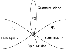
Figure 1: Single electron transistor device of Ref. [Oreg and Goldhaber-Gordon, 2003]. The two channels that hybridize with the dot are: (i) quantum island, and (ii) a linear combination of the electron channels $\Psi_{l}$ and $\Psi_{r}$ of the two Fermi liquid reservoirs.

Furthermore, as recent experiments reported in Ref. Watson et al., 2003 have realized a ”spin battery”, the two-channel Kondo device can be probed by spin transport as well. The ”spin battery”, which works by using adiabatic pumping of a chaotic cavity, provides a source for spin-bias which is controlled by the pumping frequency Mucciolo et al. (2002) and by spin-orbit interaction effects Sharma and Brouwer (2003) in the cavity.

The two-channel Kondo model that describes the low energy physics in the above mentioned system has several distinctive non-Fermi liquid features: (i) a logarithmic temperature dependence of the specific heat and magnetic susceptibity, (ii) a non-zero ground state entropy of magnitude $\frac{1}{2}\ln 2$. A simple description that captures these features is given in the language of abelian bosonization Emery and Kivelson (1992); Maldacena and Ludwig (1997); Jinwu Ye (1997); Zarand and von Delft (2000) by introducing new spinor excitations that are non-locally related to the conduction electrons. In the treatment of Ref. Emery and Kivelson, 1992, the Hamiltonian at the fixed point is written in terms of $C$-spinor degrees of freedom and a local fermion $\hat{d}$ representing the spin impurity. The entropy of the ground state that develops below the Kondo temperature, is associated with a local real (Majorana) fermion $\hat{d}+\hat{d}^{\dagger}$ that decouples from the conduction sea at the two-channel Kondo fixed point. The $C$-spinor of the “spin-flavour” sector couples to the local Majorana fermion $i[\hat{d}^{\dagger}-\hat{d}]$ only through the linear combination $C_{X}+C_{X}^{\dagger}$. The strength of this coupling is determined by the Kondo temperature $T_{K}$. This effective coupling implies that the phase variable $\hat{\theta}_{X}$ (conjugate to the difference in the number of spins between the two channels $\hat{N}_{X}$) is fixed at the bottom of a cosine potential well with a depth $T_{K}$. As a result, when the coupling is sufficiently strong ($T_{K}\gg T$), eigenstates of the fixed point Hamiltonian contain phase coherent superpositions of states with the same number of total spin but different numbers of spins in the two channels Zarand and von Delft (2000).

In this paper anomalous effects are shown in spin transport in the aforementioned quantum dot system, because of non-Fermi liquid physics near the two-channel Kondo fixed point. The predicted effects are: (i) A perfect spin conductance for isotropic Kondo coupling to the two channels, when the charge conductance is made negligible by asymmetrically coupling the right and left Fermi liquid reservoirs to the quantum dot. (ii) A sharp change from spin conducting to spin insulating behavior when the Kondo couplings are made anisotropic, i.e., there exists an anisotropy-dependent energy scale $T_{A}$ such that for $T\ll T_{A}$ the system has vanishing spin conductance. Based on the picture mentioned above, a heuristic understanding of this behavior may be arrived at as follows. When $T_{A}=0$ and $\hat{\theta}_{X}$ is a good quantum operator, a spin-bias $\lambda$ across one of the channels transforms the phase $\hat{\theta}_{X}\to\hat{\theta}_{X}+\lambda t/2$. In the phase representation the current operator is $\partial_{t}\hat{\theta}_{X}/2\pi$, and we immediately obtain a quantized spin-conductance in units of $\hbar/4\pi$. In the presence of anisotropy in the Kondo couplings, the ground state of the system is qualitatively different: the strongly coupled channel forms a singlet with the dot-spin, and $\hat{\theta}_{X}$ is no longer a good quantum operator. Therefore, the system is a spin insulator for energy scales below $T_{A}$, determined by the channel anisotropy. In what follows, we derive these results.

The modified single electron transistor can be described in terms of electron channels in the two Fermi liquid reservoirs $\Psi_{l,r}(x)$ and in the large quantum island $\Psi_{2}(x)$ (see Fig. 1), that hybridize with the spin-1/2 quantum dot. As we are interested in the low-energy physics, we linearize the electron excitation spectrum, and using open boundary conditions at the site of the single electron transistor ($x=0$) write the fields as chiral left-moving fermions. Only a linear combination $\psi_{1}(x)=\Psi_{l}(x)\sin\theta_{0}+\Psi_{r}(x)\cos\theta_{0}$ couples to the spin of the quantum dot at $x=0$, while the independent field $\psi_{0}(x)=\Psi_{l}(x)\cos\theta_{0}-\Psi_{r}(x)\sin\theta_{0}$ decouples Pustilnik et al. . The angle $\theta_{0}=\tan^{-1}[t_{l}/t_{r}]$ is dependent on the (real) tunneling amplitudes to the left ($t_{l}$) and right ($t_{r}$) Fermi liquid reservoirs.

The low-energy behavior of the above mentioned device, when the charge fluctuations in the quantum island are neglected, is that of the two-channel Kondo problem Oreg and Goldhaber-Gordon (2003); Florens and Rosch . In terms of chiral (left moving) Dirac fermions $\psi_{1,2}(x)$ Fabrizio and Gogolin (1995); Zarand and von Delft (2000) we can write the Hamiltonian ($\hbar=1$):

$$\cal{H} = \sum_{j=1,2}\sum_{\sigma=\uparrow,\downarrow}\int dx\;\psi^{\dagger}_{j\sigma}(x)\;iv\;\partial_{x}\psi_{j\sigma}(x)$$ (1)

$$- \sum_{j=1,2}\sum_{\sigma\sigma^{\prime}}J_{j}\vec{S}\cdot\psi^{\dagger}_{j\sigma^{\prime}}(0)\frac{\vec{\tau}_{\sigma^{\prime}\sigma}}{2}\psi_{j\sigma}(0).$$

Here, $\vec{S}$ represents the spin-1/2 degree of freedom of the quantum dot, $\vec{\tau}$ are the Pauli matrices, and $v$ is the Fermi velocity. Applying a spin chemical potential difference $\lambda$ between the right and left Fermi liquid leads adds a term

$$H_{\lambda} = \lambda\sum_{\sigma=\uparrow,\downarrow}\frac{\tau^{3}_{\sigma\sigma}}{2}\left[N_{l\sigma}-N_{r\sigma}\right],$$ (2)

$$N_{l\sigma} = \int_{-L/2}^{L/2}dx\;\Psi_{l\sigma}(x)\Psi_{l\sigma}(x),$$ (3)

to the Hamiltonian ${\cal H}$ in Eq. (1). This can be written in terms of the operator $\psi_{1}$ that couples to the spin of the dot, and the free field $\psi_{0}$, using the relation:

$$N_{l\sigma}-N_{r\sigma} = \cos 2\theta_{0}\;[N_{1\sigma}-N_{0\sigma}]-\sin 2\theta_{0}N_{01\sigma},$$ (4)

$$N_{01\sigma} = \int dx[\psi_{0\sigma}^{\dagger}(x)\psi_{1\sigma}(x)+H.c.].$$ (5)

Having chosen the spin quantization axis, we use abelian bosonization to calculate the spin current. The four chiral fermions $\psi_{j\sigma}(x)$ can be written in terms of chiral bosons $\phi_{j\sigma}$:

$$\psi_{j\sigma}(x) = \frac{\chi_{j\sigma}}{\sqrt{2\pi a_{0}}}e^{-i\hat{\theta}_{j\sigma}}e^{-i\hat{N}_{j\sigma}\frac{2\pi}{L}x}e^{-i\phi_{j\sigma}(x)}.$$ (6)

Here $v/a_{0}$ is the bandwidth, $\hat{N}_{j\sigma}$ counts the change in the number of electrons with spin $\sigma$ in channel $j$ with respect to a free electron ground state, $\hat{\theta}_{j\sigma}$ is its conjugate phase operator, $L/2$ is the length of each channel, and the cocycles $\chi_{j\sigma}$ are required to satisfy the relations: $\{\chi_{j\sigma},\chi_{j^{\prime}\sigma^{\prime}}\}=2\delta_{jj^{\prime}}\delta_{\sigma\sigma^{\prime}}$. It is clear from the form of ${\cal H}$ that it can be written entirely in the spin sector (involving only the bosonic fields $\phi_{j\uparrow}-\phi_{j\downarrow}$). The only term that couples spin fields to the charge fields ($\phi_{j\uparrow}+\phi_{j\downarrow}$) is the $N_{01\sigma}$ term in the external perturbation $H_{\lambda}$.

In the experimental set-up the parameter $\theta_{0}$ can be made small. As a result it is convenient to write the spin current operator $I_{\rm sp}$ as a sum of two distinct contributions:

$$I_{\rm sp} = \frac{1}{2}\frac{d}{dt}\tau^{3}_{\sigma\sigma}[N_{l\sigma}-N_{r\sigma}]=I_{11}+I_{01}$$ (7)

$$I_{11} = \cos 2\theta_{0}\frac{1}{2}\frac{d}{dt}\sum_{\sigma}\tau^{3}_{\sigma\sigma}N_{1\sigma}$$ (8)

$$I_{01} = \sin 2\theta_{0}\frac{1}{2}\frac{d}{dt}\sum_{\sigma}\tau^{3}_{\sigma\sigma}[\psi^{\dagger}_{0\sigma}\psi_{1\sigma}+H.c.]$$ (9)

It is important to note that the two-channel Kondo Hamiltonian (1) has spin- and charge- sectors separated, and also that the field $\psi_{0}$ does not couple to the dot spin. Therefore, the spin current $\langle I_{\rm sp}\rangle$ can only depend on even powers of $\sin 2\theta_{0}$. This is easy to see for $\langle I_{11}\rangle$, since $I_{11}$ depends only on the spin sector the lowest order contribution is quadratic in $V\sin 2\theta_{0}$. For $\langle I_{01}\rangle$, the lowest order contribution is from $N_{01}$ term of $H_{\lambda}$. This is apparently of order $V\sin^{2}2\theta_{0}$, however, it can easily be shown to vanish Pustilnik et al. . It follows then, that there is no contribution to the zero bias conductance upto terms of order $\sin^{2}2\theta_{0}$. Therefore, if one arranges the experimental set-up such that $\sin\theta_{0}\ll 1$, we can neglect these contributions altogether. As we show below, the remaining dominant contribution to the spin current shows scaling behavior with temperature and externally applied spin bias $\lambda$. The $\theta_{0}$ independent spin current is in marked contrast to the charge current (in response to a charge-bias) that has been shown to have a peak value of $2e^{2}/h\sin^{2}2\theta_{0}$ Pustilnik et al. . In what follows, we shall calculate the spin current $\langle I_{\rm sp}\rangle$ in response to the externally applied bias $H_{\lambda}=\sum_{\sigma}\lambda\frac{\tau^{3}_{\sigma\sigma}}{2}N_{1\sigma}.$ We begin by introducing charge (${\rm c}$), spin (${\rm s}$), flavour (${\rm f}$), and spin-flavour (${X}$) bosons:

$$\Phi_{\rm c(s)} = \frac{1}{2}\sum_{j=1,2}[\phi_{j\uparrow}\pm\phi_{j\downarrow}],\,\Phi_{{\rm f}}=\frac{1}{2}\sum_{\beta}[\phi_{1\beta}-\phi_{2\beta}],$$

$$\Phi_{X} = \frac{1}{2}[\phi_{1\uparrow}-\phi_{1\downarrow}-\phi_{2\uparrow}+\phi_{2\downarrow}].$$ (10)

Similar relations hold for defining the corresponding zero-mode number $\hat{N}_{\rm c,s,f,X}$ and phase operators $\hat{\theta}_{\rm c,s,{f},X}$. The physics near the two-channel-Kondo fixed point is conveniently described in terms of a new basis of $C$-spinors Emery and Kivelson (1992); Maldacena and Ludwig (1997):

$$C_{\alpha}(x)=\frac{\hat{\chi}_{\alpha}}{\sqrt{2\pi a_{0}}}e^{-i\hat{\theta}_{\alpha}}e^{-i\hat{N}_{\alpha}2\pi x/L}e^{-i\Phi_{\alpha}(x)},$$ (11)

where $\alpha={\rm c,s,f,X}$. Following Ref. [Emery and Kivelson, 1992], a unitary transform $U={\rm exp}[iS^{z}\Phi_{\rm s}(0)]$ yields the Hamiltonian ${\cal H}^{\prime}=U{\cal H}U^{\dagger}$ which has spin (${\rm s}$) and spin-flavour (${X}$) sectors decoupled from the charge (${\rm c}$) and flavour (${\rm f}$) sectors. The Hamiltonian ${\cal H}^{\prime}$ can be written in terms of the $C$-spinors and the local fermion $\hat{d}=\chi_{\rm s}e^{i\hat{\theta}_{\rm s}}S^{-}$, where $\hat{\theta}_{\rm s}$ is the phase conjugate to the total spin number operator $\hat{N}_{\rm s}$,

$${\cal H}^{\prime} = U{\cal H}U^{\dagger}$$ (12)

$$= i\int dx\;v\left[C_{X}^{\dagger}(x)\partial_{x}C_{X}(x)+C_{\rm s}(x)\partial_{x}C_{\rm s}(x)\right]$$

$$+ \Big{\{}\frac{J_{1}}{\sqrt{2\pi a_{0}}}\hat{d}\;C_{X}^{\dagger}(0)+\frac{J_{2}}{\sqrt{2\pi a_{0}}}\hat{d}\;C_{X}(0)+H.c.\Big{\}}$$

$$+ \frac{1}{2}\left[J_{1}+J_{2}-4\pi v\right][\hat{d}^{\dagger}\hat{d}-\frac{1}{2}]:C_{\rm s}^{\dagger}(0)C_{\rm s}(0):$$

$$+ \frac{1}{2}\left[J_{1}-J_{2}\right][\hat{d}^{\dagger}\hat{d}-\frac{1}{2}]:C_{X}^{\dagger}(0)C_{X}(0):$$

In the absence of channel anisotropy $J_{1}=J_{2}$, the above two-channel Kondo system flows to a fixed point with the critical coupling $[J_{1}+J_{2}]/2=J^{*}=2\pi v$, Fabrizio and Gogolin (1995); Jinwu Ye (1997) which gives the Kondo temperature $J^{*}/\sqrt{2\pi a}\equiv\sqrt{T_{K}}$, where $v/a$ is the reduced bandwidth. We restrict our attention to the effective Hamiltonian ${\cal H}_{\rm 2CK}$ that contains all the relevant (in the renormalization group sense) operators near the two-channel Kondo fixed point Affleck et al. (1992). This can be conveniently written by introducing Majorana (real) fermions

$$\hat{a} = \frac{\hat{d}-\hat{d}^{\dagger}}{i\sqrt{2}},\,\,\hat{b}=\frac{\hat{d}+\hat{d}^{\dagger}}{\sqrt{2}}$$

$$\eta_{a} = \frac{[C_{X}(x)+C_{X}^{\dagger}(x)]}{\sqrt{2}},\,\,\eta_{b}=\frac{[C_{X}(x)-C_{X}^{\dagger}(x)]}{\sqrt{2}}.$$ (13)

The effective Hamiltonian:

$${\cal H}_{\rm 2CK} = \frac{1}{2}\int\!dx\;\sum_{j=a,b}\eta_{j}(x)\left[iv{\partial_{x}}\right]\eta_{j}(x)$$ (14)

$$- i2\sqrt{T_{K}}\;\hat{a}\;\eta_{a}(0)-i2\sqrt{T_{A}}\;\hat{b}\eta_{b}(0),$$

valid for energy scales below the Kondo temperature $T_{K}$, also contains the crossover energy scale associated with channel anisotropy $T_{A}$. This energy scale is related to the Kondo couplings in Eq. (1) as Pustilnik et al. $T_{A}\sim[2\pi v(J_{1}-J_{2})/(J_{1}+J_{2})^{2}]^{2}T_{K}$. The external spin-bias in the basis of $C$-spinors

$$H_{\lambda}^{\prime} = UH_{\lambda}U^{\dagger}=\frac{\lambda}{2}N_{X}-\frac{\lambda}{2}S^{z},$$ (15)

where $N_{X}=\int dx:C_{X}^{\dagger}(x)C_{X}(x):$ and $S^{z}=-i\hat{a}\hat{b}$ in terms of the local Majorana fermions. The corresponding spin current operator is

$$I^{\prime}_{\rm sp}=UI_{\rm sp}U^{\dagger}=\frac{1}{2}\frac{d}{dt}\left[N_{X}+i\hat{a}\hat{b}\right]$$ (16)

A transformation $C_{X}\to C_{X}e^{i\lambda(x-vt)/2}$ removes the first term of $H_{\lambda}^{\prime}$, and corresponds to a change in the chemical potential of the $C_{X}$ fermions. We will calculate the energy dependent phase shift of these fermions as they scatter off the local Majorana fermions. As these are left-movers we choose the incoming states to the right of the impurity ($x>0$). The equations of motion of these fermions are:

$$\partial_{t}\eta_{a}(x) = v\partial_{x}\eta_{a}(x)+\delta(x)\sqrt{T_{K}}\hat{a}$$ (17a)

$$\partial_{t}\hat{a} = -\frac{1}{2}\lambda\hat{b}-2\sqrt{T_{K}}\eta_{a}(0)$$ (17b)

$$\partial_{t}\hat{b} = +\frac{1}{2}\lambda\hat{a}+2\sqrt{T_{A}}\eta_{b}(0)$$ (17c)

Integrating across the impurity gives us:

$$2\sqrt{T_{K}}\hat{a} = \eta_{a}(0^{-})-\eta_{a}(0^{+})$$ (18a)

$$2\sqrt{T_{A}}\hat{b} = \eta_{b}(0^{+})-\eta_{b}(0^{-})$$ (18b)

$$2\partial_{t}\hat{a} = -\lambda\hat{b}-2\sqrt{T_{K}}[\eta_{a}(0^{+})+\eta_{a}(0^{-})]$$ (18c)

$$2\partial_{t}\hat{b} = \lambda\hat{a}+2\sqrt{T_{A}}[\eta_{b}(0^{+})+\eta_{b}(0^{-})]$$ (18d)

Introducing the scattering matrix ${\cal S}$ allows us to write the outgoing fields near the impurity

$$\eta_{Y=a,b}(0^{-})=\sum_{Y^{\prime}=a,b}\sum_{k}{\cal S}_{YY^{\prime}}(k)\eta_{Y^{\prime},k}$$ (19)

where $\eta_{Y,k}$ is the $k$-th mode of the incoming field $\eta_{Y}(0^{+})$. Using this ansatz in Eqs. (18) we obtain:

$${\cal S}_{aa} = 1+\frac{(e^{i\delta_{a}}-1)}{\left[1+\left(\frac{\lambda}{8\sqrt{T_{K}}}\right)^{2}(e^{i\delta_{a}}-1)(e^{i\delta_{b}}-1)/T_{A}\right]}$$ (20)

$${\cal S}_{ba} = \frac{\lambda}{2}\sqrt{\frac{T_{A}}{T_{K}}}\frac{(e^{i\delta_{b}}-1)}{4T_{A}}{\cal S}_{aa},$$ (21)

$$e^{i\delta_{a}} = \frac{ivk+2T_{K}}{ivk-2T_{K}},\,\,\,e^{i\delta_{b}}=\frac{ivk+2T_{A}}{ivk-2T_{A}}.$$ (22)

The scattering phase shift of the $C_{X}$ fermion at the two-channel Kondo fixed point (when $T_{A}=0=\lambda$) is easily verified to be $\delta_{a}(k=0)=\pi,\,\delta_{b}=0$, in accordance with Ref. [Maldacena and Ludwig, 1997]. The spin current (16) can be written in terms of the incoming and outgoing fields at the impurity, using (18), and evaluated at finite bias and temperature:

$$\langle I_{\rm sp}\rangle = v\left\langle C_{X}^{\dagger}(0^{+})C_{X}(0^{+})-C_{X}^{\dagger}(0^{-})C_{X}(0^{-})\right\rangle$$ (23)

$$= \frac{v}{4\pi}\int dk\;{\rm Re}\left[{\cal S}_{aa}^{*}{\cal S}_{bb}-1-|{\cal S}_{ab}|^{2}\right]$$

$$\times \left[f(vk-\lambda/2)-f(vk+\lambda/2)\right].$$

Here $f(x)$ is the Fermi function, and the integral is limited by the upper momentum cut-off $T_{K}/v$.

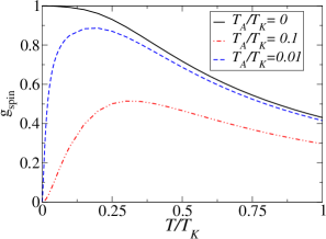
Figure 2: Differential spin conductance $g_{\rm sp}$ as a function of temperature for three different values of the channel anisotropy energy scale $T_{A}$. Two-channel Kondo behavior is evident for $T_{A}\ll T\ll T_{K}$, while one-channel Kondo behaviour for $T\ll T_{A}$.

At the two-channel Kondo fixed point ($T_{A}=0$) the current at low bias $\lambda\ll T_{K}$,

$$\langle I_{\rm sp}\rangle \equiv \frac{\lambda}{4\pi}{g_{\rm sp}}=-\frac{\lambda}{4\pi}\int dk\;\sin^{2}\left(\frac{\delta_{a}}{2}\right)\frac{df(vk)}{dk}$$

$${g_{\rm sp}} = \frac{2T_{K}}{\pi T}\Psi^{\prime}\left(\frac{1}{2}+\frac{2T_{K}}{\pi T}\right)\approx 1-\frac{1}{3}\left(\frac{\pi T}{2T_{K}}\right)^{2}.$$ (24)

Here $\Psi^{\prime}(x)$ is the derivative of the psi function, and the last expression is valid for $T\ll T_{K}$. The quantized spin conductance $g_{\rm sp}$ is the signature of the two-channel Kondo fixed point. Deviations from the fixed point, because of $T_{A}\neq 0$ and also because of an external magnetic field at the quantum dot site, decrease the zero-bias spin conductance: At $T=0$ a non-zero $T_{A}$ leads to a vanishing zero-bias conductance, while

$$g_{\rm sp} = -\int dk\;\sin^{2}\left(\frac{\delta_{a}-\delta_{b}}{2}\right)\frac{df(vk)}{dk}$$ (25)

$$\approx \left(1-\frac{T_{A}^{2}}{T_{K}^{2}}\right)\zeta(2)\left(\frac{T}{T_{A}}\right)^{2},\,{\rm for}\,T\ll T_{A}\ll T_{K}.$$

The full temperature dependence is plotted in Fig. 2.

The role of local magnetic field is similar to that of channel anisotropy. The zero-bias spin conductance in the presence of a local magnetic field with Zeeman energy $\lambda_{h}$ is obtained by replacing the spin-bias $\lambda\to\lambda_{h}$ in the phase shifts $\delta_{a,b}$. The Zeeman energy corresponding to the crossover energy $T_{A}$ is then found to be $\lambda_{h}\sim\sqrt{T_{A}T_{K}}$. Note that we have shown the zero temperature behavior of spin conductance to be identical to that of the impurity entropy Fabrizio et al. (1995). Therefore, the presence of a degenerate ground state at the two-channel Kondo fixed point implies perfect conductance. Also, note that the temperature dependence of the spin conductance in this device, for $T_{A}=0$, is similar to that of charge conductance in a one-channel Kondo set-up Kaminski et al. (2000), i.e., in the absence of the quantum island.

In conclusion, we have calculated the spin current through the two-channel-Kondo quantum dot device of Ref. Oreg and Goldhaber-Gordon, 2003 for temperature and spin-bias smaller than the Kondo temperature $T_{K}$. We have shown that the spin conductance is simply related to the phase shift of the $C_{X}$ spinor, and that the two-channel Kondo fixed point can be identified by tuning the device parameters to obtain perfect spin conductance. Deviations from the fixed point, because of channel anisotropy and external magnetic field at the quantum dot site, are shown to lead to a spin insulator.

This work was supported by the Packard foundation.

References

- Hewson (1993) A. C. Hewson, The Kondo Problem to Heavy Fermions (Cambridge University Press, 1993).
- Ph Nozieres and Blandin (1980) Ph Nozieres and A. Blandin, J. Phys. (Paris) 41, 193 (1980).
- Goldhaber-Gordon, et al. (1998a) D. Goldhaber-Gordon, et al., Nature 391, 156 (1998a).
- Cronenwert et al. (1998) S. M. Cronenwert, T. H. Oosterkamp, and L. P. Kouwenhoven, Science 540, 281 (1998).
- Goldhaber-Gordon, et al. (1998b) D. Goldhaber-Gordon, et al., Phys. Rev. Lett. 81, 5225 (1998b).
- van der Wiel et al. (2000) W. G. van der Wiel et al., Science 289, 2105 (2000).
- Nygard et al. (2000) J. Nygard, D. H. Cobden, and P. E. Lindelof, Nature 408, 342 (2000).
- Liang et al. (2002) W. Liang, M. Bockrath, and H. Park, Phys. Rev. Lett. 88, 126801 (2002).
- Pustilnik and Glazman (2001) M. Pustilnik and L. I. Glazman, Phys. Rev. Lett. 87, 216601 (2001).
- Affleck and Simon (2001) I. Affleck and P. Simon, Phys. Rev. Lett. 86, 2854 (2001).
- Kaminski et al. (1999) A. Kaminski, Y. V. Nazarov, and L. I. Glazman, Phys. Rev. Lett. 83, 384 (1999).
- Kaminski et al. (2000) A. Kaminski, Y. V. Nazarov, and L. I. Glazman, Phys. Rev. B 62, 8154 (2000).
- (13) X. G. Wen, eprint cond-mat/9812431v2.
- Coleman et al. (2001) P. Coleman, C. Hooley, and O. Parcollet, Phys. Rev. Lett. 86, 4088 (2001).
- Rosch et al. (2001) A. Rosch, J. Kroha, and P. Wölfle, Phys. Rev. Lett. 87, 156802 (2001).
- Fabrizio and Gogolin (1995) M. Fabrizio and A. O. Gogolin, Phys. Rev. B 51, 17827 (1995).
- (17) E. H. Kim, G. Sierra, and C. Kallin, eprint cond-mat/0202387.
- Oreg and Goldhaber-Gordon (2003) Y. Oreg and D. Goldhaber-Gordon, Phys. Rev. Lett. 90, 136602 (2003).
- (19) S. Florens and A. Rosch, eprint cond-mat/0311219.
- (20) M. Pustilnik, L. Borda, L. I. Glazman, and J. von Delft, eprint cond-mat/0309646.
- Watson et al. (2003) S. K. Watson, R. M. Potok, C. M. Marcus, and V. Umansky, Phys. Rev. Lett. 91, 258301 (2003).
- Mucciolo et al. (2002) E. R. Mucciolo, C. Chamon, and C. M. Marcus, Phys. Rev. Lett. 89, 146802 (2002).
- Sharma and Brouwer (2003) P. Sharma and P. W. Brouwer, Phys. Rev. Lett. 91, 166801 (2003).
- Emery and Kivelson (1992) V. J. Emery and S. Kivelson, Phys. Rev. B 46, 10812 (1992).
- Maldacena and Ludwig (1997) J. M. Maldacena and A. W. W. Ludwig, Nucl. Phys. B 506, 565 (1997).
- Jinwu Ye (1997) Jinwu Ye, Phys. Rev. Lett. 79, 1385 (1997).
- Zarand and von Delft (2000) G. Zarand and J. von Delft, Phys. Rev. B 61, 6918 (2000).
- Affleck et al. (1992) I. Affleck, A. W. W. Ludwig, H. B. Pang, and D. L. Cox, Phys. Rev. B 45, 7918 (1992).
- Fabrizio et al. (1995) M. Fabrizio, A. O. Gogolin, and Ph. Nozierés, Phys. Rev. Lett. 74, 4503 (1995).