Transition matrix Monte Carlo method for quantum systems

Abstract

We propose an efficient method for Monte Carlo simulation of quantum lattice models. Unlike most other quantum Monte Carlo methods, a single run of the proposed method yields the free energy and the entropy with high precision for the whole range of temperature. The method is based on several recent findings in Monte Carlo techniques, such as the loop algorithm and the transition matrix Monte Carlo method. In particular, we derive an exact relation between the DOS and the expectation value of the transition probability for quantum systems, which turns out to be useful in reducing the statistical errors in various estimates.

I Introduction

The Monte Carlo method for classical and quantum lattice models has been improved dramatically since the proposal of the Metropolis methodMetropolis . The introduction of the extended ensemble, being one of the ideas that enhanced the Monte Carlo method, is characterized by a random walker traveling in the energy space. The most well-known methods among the ones based on the extended ensemble is the multicanonical method BergN ; Lee . In this method, one can obtain the density of states (DOS) from the histogram of visiting frequency at each value of the energy. Since the random walk in the extended ensemble methods is typically biased in a complicated way, the scaling property of the the traveled distance of the walker deviates from that of the free random walk, i.e., $R\sim\sqrt{t}$. This means that the random-walk nature of the method does not necessarily guarantee a quick equilibration. However, in many important application, it turns out that the random walker can still travel the whole range of the energy within a reasonable computational time, i.e., a computational time bounded by some polynomial in the system size. Therefore, the method is quite useful for models that has a first-order phase transition and/or ones that have local minima in the free energy. In addition, the direct calculation of the DOS makes it possible to calculate the absolute value of the free energy of a given system with high precision. Another advantage of this type of approach is that thermal averages of various quantities can be obtained for the whole range of the temperature from only a single run of simulation. While the early versions of extended ensemble methods still suffered from a slow diffusion, even this problem was removed recently by the acceleration method proposed by Wang and Landau (WL) WangL , in which the random walker is forced to move away whenever it lingers about a place for a long time.

For many important models, classical or quantum, it was found that the loop/cluster algorithm SwendsenW ; Evertz is so efficient that the simulation can be done with no (or negligible) difficulty of slowing down at any temperature. However, since the algorithm is originally designed for a simulation at a fixed temperature, one cannot obtain from a single run the whole temperature dependence of various quantities nor can one estimate the free energy. Therefore, it is natural to wonder if the loop/cluster algorithm can be used together with the extended ensemble methods. An apparent obstacle is that the energy in the quantum case is not defined so that constructing a histogram on it is straightforward and meaningful. Janke and Kappler proposedJankeK that in the cluster algorithm for classical spin systems one can use the number of graph elements (such as bonds in the Swendsen-Wang algorithm) instead of the energy for constructing the histogram, showing a way for combining the extended ensemble method and the cluster algorithm for classical spin systems. Furthermore, two of the present authors demonstratedYamaguchiK the enhancement of the efficiency achieved with the use of the WL method, and also suggested that the resulting framework can be generalized to quantum systems. Later, the application to the quantum systems was done with a different formulation by Troyer, Wessel and Alet TroyerWA , who also showed the efficiency of the resulting algorithm.

In the present paper, we propose that a further improvement can be achieved for quantum models by using the broad-histogram (BH) relation for estimating the DOS. The idea has been partially described in our previous paper YamaguchiKO for the classical models. For the Ising models, it was pointed out Oliveira1 that a ratio of the densities of states at two neighboring values of the energy can be expressed in terms of the microcanonical averages of the numbers of distinct potential moves. In the application to the Ising model, the number of potential moves is nothing but the number of spins such that flipping one of them causes a change in the energy by a given amount. Since this is a macroscopic quantity, whereas the number of the visits at each value of the energy is not, we can estimate the DOS more precisely by using the relation than we do so directly from the histogram. In the case that we discuss here, our DOS is not simply the total number of states. Therefore we have to use the generalized form of the transition matrix Monte Carlo method WangTS . In what follows, we describe the method specialized for quantum systems.

II The outline of the algorithm

The simulation consists of two stages. In the first stage we perform short runs using the WL method for obtaining a working estimate of the DOS. As explained below, each run in the first stage is characterized by a parameter called the modification factor, which controls the adoptive change of the fictitious weight of the random walk. A stronger control is imposed on earlier runs whereas a weaker control for the latter runs. Because of this adoptively changing weight, the microcanonical ensemble obtained in each run of the first stage deviates from the correct one. This leads to some systematic error. However, we need unbiased estimates of microcanonical averagesNote1 because we use them for obtaining the DOS from the BH relation. Therefore, in the second stage we perform a single long run with the weight fixed to the one obtained in the first stage. This is in contrast to the ordinary WL method where the outcome of the first stage is taken as the final estimate of the DOS. The organization of the whole simulation is schematically depicted in Fig. 1. We will show this two-stage procedure gives more precise results for quantum systems than the one-stage procedure of the WL method described in TroyerWA , within the same amount of the total CPU time.

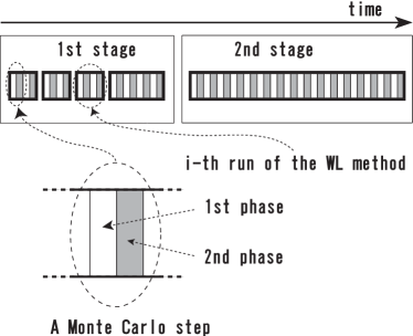
Figure 1: The organization of a set of simulation.

A little more specifically, the whole simulation can be described as follows. We construct a histogram of the expansion order or the number of active vertices, which we denote as $n$, instead of the histogram of the energy. Accordingly, the fictitious weight $f(n)$ is introduced as a function of $n$, rather than the energy. The Monte Carlo dynamics is defined so that the detailed balance holds for this weight. We start the first run of the first stage by setting the weight $f(n)$ to be constant, i.e., $f(n)=1$ for all $n$. At the beginning of each run, the counter (or the histogram), $H(n)$, of visits to the value $n$ is set to be 0 while $f(n)$ is not reset except at the beginning of the first run. For the $i$-th run we use the modification factor $\lambda_{i}\equiv e^{-2^{-i}}$. Every time the random walker visit a state with $n(S)=n$, $f(n)$ is replaced by $\lambda_{i}f(n)$ in order to penalize the random walker staying at this value of $n$. At the same time, $H(n)$ is increased by one. The $i$-th run is terminated when the histogram becomes flat. To be specific, the flatness condition is

$$H(n)\geq 0.8\times\sum_{n^{\prime}}H(n^{\prime})/\sum_{n^{\prime}}1$$

for all $n$. Since the first stage is only for obtaining a working estimate of the DOS, we stop when $-\ln\lambda_{i}<10^{-5}$ whereas in the original WL method $-\ln\lambda_{i}<10^{-8}$ was used instead. At the end of the first stage, $(f(n))^{-1}$ is approximately proportional to the generalized DOS discussed below. In the second stage, we do the same as the first stage but with a longer run and with $f(n)$ fixed to be the result of the first stage. In this way, we can compute non-biased microcanonical averages of various quantities in the second stage.

In both the first and the second stages, the update of the configuration is done using the loop update if the update does not involve a change in $n$. Other similar algorithms such as the directed loop algorithm SS can be used as well, and the generalization is straight-forward. The choice, however, is only of the secondary importance for the applications to the models without the magnetic field as considered in the present paper. For the loop algorithm, there are two formulations; one is based on the continuous imaginary time and the other is the discrete imaginary time. Although the difference in the efficiencies of two formulations is minor, in the present paper we have used the discrete time formulation following Troyer, Wessel and AletTroyerWA . In what follows, we reformulate their algorithm, use it for deriving the BH relation, and describe how the relation is used in the second stage of the simulation.

The systematic error due to the discretization in the discrete time formulation can be removed by starting from the high-temperature series expansion Sandvik rather than the path-integral representation. Therefore, we start with expressing the partition function $Z$ as a high-temperature series expansion truncated at the $L$-th order,

$$Z_{0} = {\rm Tr}e^{-\beta{\cal H}}\approx\sum_{n=0}^{L}\frac{\beta^{n}}{n!}{\rm Tr}\left(-{\cal H}\right)^{n}$$ (1)

$$= \sum_{n=0}^{L}\beta^{n}\frac{L!}{(L-n)!}\sum_{\{\gamma_{l}\}\atop(\sum\gamma_{l}=n)}{\rm Tr}\prod_{l}(-{\cal H})^{\gamma_{l}}$$

$$= \sum_{n=0}^{L}\beta^{n}\,\omega(n)\,,$$

where $\beta$ is inverse temperature $1/k_{B}T$, $k_{B}$ is Boltzmann’s constant, and $\gamma_{l}$ is a variable that takes on $0$ or $1$. The high-temperature expansion coefficient, $\omega(n)$, is here regarded as the generalized DOS for the series order $n$. When the Hamiltonian is expressed as a sum of $M$ local interaction terms as ${\cal H}=\sum_{b=1}^{M}{\cal H}_{b}$, the generalized DOS is given by

$$\omega(n)=\frac{(L-n)!}{L!}\sum_{\{\gamma_{l,b}\}\atop\left({\sum_{l,b}\gamma_{l,b}=n\atop\sum_{b}\gamma_{l,b}\leq 1}\right)}\sum_{\{\psi_{l}\}}\prod_{l,b}\langle\psi_{l+1}|(-{\cal H}_{b})^{\gamma_{l,b}}|\psi_{l}\rangle.$$ (2)

We can simplify the notation by defining a vertex, $v$, as a pair of indices $l$ and $b$, i.e., $v=(l,b)$. Several other symbols are also introduced for simplification of the notation: $\Gamma\equiv\{v\,|\,\gamma_{v}=1\}$, $\Psi\equiv(\psi_{1},\psi_{2},\cdots,\psi_{L})$, $\Psi_{v}\equiv(\psi_{l+1},\psi_{l})$, $u(\Psi_{v})\equiv\langle\psi_{l+1}|(-H_{b})|\psi_{l}\rangle$, $S\equiv(\Psi,\Gamma)$, and $n(S)\equiv|\Gamma|$. As a result, we can rewrite the generalized DOS as

$$\omega(n)=\sum_{{S\atop(n(S)=n)}}U(S)$$ (3)

where

$$U(S)\equiv\frac{(L-n(S))!}{L!}\prod_{v\in\Gamma}u(\Psi_{v})\prod_{v\notin\Gamma}\Delta(\Psi_{v}).$$ (4)

Here, $\Delta(\Psi_{v})\equiv\delta_{\psi_{l+1},\psi_{l}}$. By comparing these expressions to those in YamaguchiK it is natural to identify $n$ as the number of graph elements. Here we call a vertex $v$ for which $\gamma_{v}=1$ an active vertex.

We then replace the factor $\beta^{n}$ in (1) by an adjustable function $f(n)$, which makes the simulated partition function to be

$$Z=\sum_{n=0}^{L}f(n)\omega(n)=\sum_{S}W(S)$$

with the weight of the state $S$ being

$$W(S)=f(n(S))U(S).$$ (5)

In the first stage, the function $f(n)$ is adaptively modified so that the probability of having $n(S)$ to be independent of $n$. In other words, in the first stage we try to make $f(n)\omega(n)$ constant by adjusting $f(n)$. This goal is achieved by the use of the WL method. As a result, we obtain $\omega(n)$ as the inverse of $f(n)$.

III The first phase and the BH relation

The algorithm used for updating $S$ can be viewed as the dual Monte Carlo KandelDomany ; KawashimaG1995a . Namely, by regarding the variable $\gamma_{v}$ as a graph element, analogous to the bond in the Swendsen-Wang algorithm, one can establish a correspondence between the present algorithm and the Swendsen-Wang algorithm. One step in a dual Monte Carlo simulation consists of two phases; the “graph” $\Gamma$ is updated in the first phase with “spin configuration” $\Psi$ being fixed and the $\Psi$ is updated in the second phase with fixed $\Gamma$. While the first phase changes $n$, the latter does not. In what follows, we describe updating of $\Gamma$ and show how to estimate $\omega(n)$ based on estimates of macroscopic quantities. The second phase, i.e., how the update $\Psi$ with fixed $n$, is described in the next section.

In order to relate $\omega(n)$ to the microcanonical averages of some macroscopic quantities, we consider an arbitrary function $T(S^{\prime}|S)$ that satisfies

$$T(S^{\prime}|S)W(S)=T(S|S^{\prime})W(S^{\prime}).$$ (6)

While $T(S^{\prime}|S)$ could be the transition probability from $S$ to $S^{\prime}$, in which case the above equation is nothing but the detailed balance condition, it does not have to be so for the derivation of the BH relation. We sum up each side of the above equation over such $S$ and $S^{\prime}$ that $n(S)=n$ and $n(S^{\prime})=n^{\prime}$, yielding

$$\langle T(n^{\prime}|S)\rangle_{n}f(n)\omega(n)=\langle T(n|S^{\prime})\rangle_{n^{\prime}}f(n^{\prime})\omega(n^{\prime})$$ (7)

where

$$T(n^{\prime}|S)\equiv\sum_{S^{\prime}\atop(n(S^{\prime})=n^{\prime})}T(S^{\prime},S),$$

and $\langle\cdots\rangle_{n}$ is the microcanonical average, i.e.,

$$\langle Q(S)\rangle_{n}\equiv\left.\sum_{S\atop(n(S)=n)}Q(S)\right/\sum_{S\atop(n(S)=n)}1.$$

For the derivation of the BH relation, we only have to consider the case where $S^{\prime}$ and $S$ have the same spin configuration $\Psi$ in common. Then, the procedure for generating $S^{\prime}=(\Psi,\Gamma^{\prime})$ from $S=(\Psi,\Gamma)$ is as follows:

1.

Generate an integer $l$ ($1\leq l\leq L$) uniform-randomly.

2.

If $\gamma_{l}=0$, generate an integer $b$ ($1\leq b\leq M$) uniform-randomly, and change $\Gamma$ into $\Gamma^{\prime}\equiv\Gamma\cup\{v\}$ (i.e., activate $v$) with the probability $p_{v}^{+}(S)$ where $v\equiv(l,b)$.

2’.

If $\gamma_{l}=1$, change $\Gamma$ into $\Gamma^{\prime}\equiv\Gamma\backslash\{v\}$ (i.e., inactivate $v$) with the probability $p_{v}^{-}(S)$ where $v$ is the vertex $(l,b)$ such that $\gamma_{l,b}=1$.

3.

Repeat 1 and 2 (or 2’) $LM$ times.

The overall transition probability corresponding to one repetition of 1 and 2 (or 2’) can be written in the form of the transition matrix as

$$T(S^{\prime}|S) = \frac{1}{L}\sum_{l}\Big{(}\delta_{\gamma_{l},0}\sum_{b}\frac{1}{M}p_{lb}^{+}(S)\Delta(\Gamma^{\prime},\Gamma\cup\{(lb)\})$$

$$+\delta_{\gamma_{l},1}\sum_{b}\delta_{\gamma_{l,b},1}p_{lb}^{-}(S)\Delta(\Gamma^{\prime},\Gamma\backslash\{(lb)\})\Big{)},$$

where some Kronecker’s delta’s have been written as $\Delta(A,B)$ instead of $\delta_{A,B}$ for clarity. In order for this transition probability to satisfy (6) with (5) and (4), $p_{v}^{\pm}$ must satisfy

$$\frac{1}{M}(L-n)\Delta(\Psi_{v})f(n)p_{v}^{+}(S)=u(\Psi_{v})f(n+1)p_{v}^{-}(S^{\prime})$$

where $n\equiv n(S)$ and $v$ is the vertex at which $S$ and $S^{\prime}$ differ from each other. The simplest choice is

$$p_{v}^{+}(S)\equiv\frac{Mu(\Psi_{v})}{L-n}\frac{f(n+1)}{f(n)}\quad\mbox{and}\quad p_{v}^{-}(S)\equiv\Delta(\Psi_{v}).$$ (8)

Note here that we do not have to make $p_{v}^{\pm}$ smaller than 1 if we only need to make $T(S^{\prime}|S)$ satisfy (6) and if $T$ does not have to be a real transition matrix. Since this is the case for obtaining the BH relation, we shall forget about the condition $p_{v}^{\pm}\leq 1$ for a time being. With (8), $T(n+1|S)$ and $T(n-1|S)$ become

$$T(n+1|S)=\frac{1}{L}\sum_{l}\delta_{\gamma_{l},0}\sum_{b}\frac{u(\Psi_{v})}{L-n}\frac{f(n+1)}{f(n)}$$

and

$$T(n-1|S)=\frac{1}{L}\sum_{l}\delta_{\gamma_{l},1}\sum_{b}\delta_{\gamma_{l,b},1}\Delta(\Psi_{v})=\frac{1}{L}(n-n_{\rm kink}),$$

where $n_{\rm kink}$ is the number of kinks, i.e., the vertices at which $\Delta(\Psi_{v})=0$. Thus we obtain from (7) for $n^{\prime}=n+1$,

$$\frac{\langle\sum_{v}\delta_{\gamma_{l},0}u(\Psi_{v})\rangle_{n}}{L-n}\,\omega(n)=(n+1-\langle n_{\rm kink}\rangle_{n+1})\,\omega(n+1).$$ (9)

We call this relation the BH relation for quantum systems. When multiplied $\omega(n+1)/\omega(n)$ for $n=0,1,2,\cdots$, this yields

$$\omega(n)=\frac{(L-n)!}{L!}\,2^{N}\,\prod_{m=1}^{n}\frac{\langle\sum_{v}\delta_{\gamma_{l},0}u(\Psi_{v})\rangle_{m-1}}{m-\langle n_{\rm kink}\rangle_{m}}\,,$$ (10)

where $\omega(0)=2^{N}$ has been used. Note that the validity of (9) and (10) does not depend on what transition probability we use in the simulation although we have used a particular form of it in deriving the relation (9). Therefore, we can use any algorithm to estimate the DOS as long as it produces the correct microcanonical ensemble.

In fact, since we have not guaranteed that $p_{v}^{+}\leq 1$ above in (8), $T(S^{\prime}|S)$ mentioned above may not serve as the transition probability. To obtain the real transition probability, we simply replace (8) by

$$p_{v}^{+}(S)\equiv\min(1,R_{n(S)})\quad\mbox{and}\quad$$

$$p_{v}^{-}(S)\equiv\min(1,R_{n(S)-1}^{-1})\Delta(\Psi_{v}),$$

with

$$R_{n}\equiv\frac{Mu(\Psi_{v})}{L-n}\frac{f(n+1)}{f(n)}.$$

This is the transition probability that is actually used in the simulation presented below.

IV The second phase

We now turn to the second phase in which the state $S=(\Psi,\Gamma)$ is updated to $S^{\prime}=(\Psi^{\prime},\Gamma)$ with $\Gamma$ fixed. This can be done by either of the loop algorithm or the worm-type algorithm. We here adopt the loop type update Sandvik99 . The weight with which $\Psi$ must be sampled is $W(\Psi,\Gamma)$. Following the general framework of the loop algorithm we decompose the weight at every active vertex $v$ in $\Gamma$ as

$$u(\Psi_{v})=\sum_{G_{v}}a(G_{v})\Delta(\Psi_{v},G_{v})$$ (11)

where $G_{v}$ is a graph and $\Delta(\Psi_{v},G_{v})$ is the function that takes on $0$ or $1$ depending on the matching between $\Psi_{v}$ and $G_{v}$. The readers are referred to Ref.KawashimaG1995b for the details of the graphs and the $\Delta$-functions. Here we only show an example for the compactness of the description. In the case of the $S=1/2$ antiferromagnetic Heisenberg model, the decomposition consists of a single term since the local Hamiltonian can be expressed as a single delta function.

$$u(\Psi_{v})=\frac{J}{2}\Delta(\Psi_{v},G_{v}^{{\rm H}})$$

where $G_{v}^{{\rm H}}$ is a horizontal graph that consists of two horizontal lines connecting $(i,l)$ to $(j,l)$ and $(i,l+1)$ to $(j,l+1)$. The function $\Delta(\Psi_{v},G_{v}^{{\rm H}})$ is defined for $v=((ij),l)$ as

$$\Delta(\Psi_{v},G_{v}^{{\rm H}})\equiv\left\{\begin{array}[]{ll}1&(\psi_{l}(i)+\psi_{l}(j)=\psi_{l+1}(i)+\psi_{l+1}(j)=0)\\ 0&(\mbox{Otherwise})\end{array}\right..$$

Here we have assumed that the state $|\psi_{l}\rangle$ is the simultaneous eigenstate of all the $z$-components of spins. Namely, $\psi_{l}(i)$ $(=\pm 1/2)$ denotes the eigenvalue of $S_{i}^{z}$ of the eigenstate $|\psi_{l}\rangle$. Therefore, the update is done by placing horizontal graphs on all the vertices in $\Gamma$, and connect the end points of horizontal lines by vertical lines to form loops, then finally flip every loop with probability 1/2. The generalization to the case where the expansion of the Hamiltonian (11) consists of multiple terms is straight-forward. In such a case, we simply choose a graph from the ones for which $\Delta(\Psi_{v},G_{v})=1$ with the probability proportional to $a(G_{v})$.

V Results

In order to see if the present procedure yields better statistics than previous methods, we calculate the spin-1/2 antiferromagnetic Heisenberg chain of ten sites. We set the initial value of the modification factor to $e^{-128}$ for the whole calculation in the paper. (For an appropriate initial value of the modification factor, see the discussions in the referencesWangL ; TroyerWA .)

We set the cut off $L$ to be 500. This limits the accessible temperature range to $T\gtrsim 0.05J$. In the first stage, it takes approximately $6\times 10^{6}$ Monte Carlo steps (MCS) before the last run with $-\ln\lambda_{i}<10^{-5}$ terminates. In the second stage of simulation, we fix $f(n)$ and let the random walker travel for $1\times 10^{8}$ MCS. The final estimate of the DOS is shown in Fig. 2.

Figure 2: The density of states for the series orders for the antiferromagnetic spin-1/2 Heisenberg chain on ten-site. The cut off of series orders is $L=500$. The first stage of simulation was performed for $6\times 10^{6}$ Monte Carlo sweeps and the second stage was calculated for $1\times 10^{8}$ Monte Carlo sweeps.

By using the DOS in Fig. 2, canonical (fixed-temperature) averages of the energy, the specific heat, the free energy, and the entropy are calculated as functions of temperature.

In Fig. 3, we show the relative error in the free energy,

$$\epsilon_{F}\equiv\left|\frac{F^{({\rm Exact})}(T)-F^{({\rm Simulation})}(T)}{F^{({\rm Exact})}(T)}\right|\,.$$

Figure 3: Relative errors of the free energy for the antiferromagnetic spin-1/2 Heisenberg chain on ten-site. The cut off of series orders is $L=500$. The solid line is the result of the Wang-Landau algorithm of the first stage, which took $6\times 10^{6}$ MCS. The dotted line represents the result of the multicanonical method in the second stage of simulation. The short dashed line is the result by using the broad histogram relation in the second stage of simulation. The dashed line is the result of Troyer et. al. TroyerWA that is drawn at the worst value.

The top solid line is the one that is obtained based on the working estimate of $\omega(n)$ resulting from the first stage that takes about $6\times 10^{6}$ sweeps. The bottom dashed line represent the one based on the final estimate of $\omega(n)$ obtained from the second stage using the estimator (10). The middle dotted line also represent the free energy based on the second stage data but without using the estimator (10). This corresponds to the standard procedure of the multicanonical simulation BergN ; Lee . Namely, the middle curve is based on the naive estimate of the DOS using the histogram itself, i.e., the estimate using the relation $\omega(n)\propto H(n)\omega^{\rm trial}(n)$ where $\omega^{\rm trial}\propto(f(n))^{-1}$ is the trial DOS estimated in the first stage and $H(n)$ is the number of visits to the value $n$ counted during the second stage simulation. The difference between the middle curve and the bottom one is as much as 1 to 2 orders of magnitude, and it clearly shows the utility of the estimator (10). The horizontal dashed line indicates the level of the largest error of the previous simulation by Troyer, Wessel and AletTroyerWA for the same system with the same size. The number of Monte Carlo sweeps performed in their simulation was the same as the second stage of our simulation. It is natural that their result is about the same position as the worst (i.e., the highest) point in the middle curve, since the last few runs in the WL method, where the modification factor is very close to one, are almost equivalent to the ordinary multicanonical simulation with fixed weight.

In order to see the system-size dependence of the efficiency, we calculate the standard deviation $\sigma$ of the specific heat per site at temperature $T=0.5J$ for various system sizes. Again, we compare three results: (1) the one based on a WL method only with the termination condition $-\ln\lambda_{i}<10^{-8}$ (denoted as “Wang-Landau” in the figure), (2) the one based on the two stage simulation with the termination condition $-\ln\lambda_{i}<10^{-5}$ for the first stage and with the naive estimation of the DOS using the histogram itself in the second stage (denoted as “multicanonical”), and (3) the same as the above but with the estimator (10) (denoted as “broad histogram”). In (2) and (3), the total number of Monte Carlo sweeps are chosen to be the same as that is spent in (1) in order to make the comparison fair. We choose $L$ and $M$ so that $L/M=50$ is fixed. With this choice the accessible temperature range is $T\gtrsim 0.05J$. 40 independent sets are performed for $M=8,12,16,20$ whereas 12 for $M=24$. The results are shown in Fig. 4.

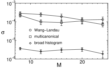
Figure 4: The system-size dependences of the standard deviation $\sigma$ for the specific heat per one site at $T=0.5J$ for the spin-1/2 antiferromagnetic Heisenberg chain. Three methods were compared: the generalized WL algorithm (circles), the combination of the multicanonical method and the generalized WL algorithm (squares), and the proposed method (diamonds). The methods spent the same MCS for each $M$. We took the $M$ and the $L$ as $(M,L)=(8,400),(12,600),(16,800),(20,1000)$. The accessible temperature range is $T\gtrsim 0.05J$. 40 sets of simulation are performed for $M=8,12,16,20$ and 12 sets for $M=24$.

The system size dependence is small. The results of the WL algorithm and the naive estimate of the DOS based on the two-stage simulation are close to each other again. The proposed method outperforms the other method by more than an order of magnitude in all the cases studied here.

VI Summary

Generalizing the histogram methodsJankeK ; YamaguchiK ; YamaguchiKO based on the graph representation, we have presented a Monte Carlo method for quantum lattice models that consists of two stages. For the method’s performance, the generalized broad histogram relation (9), proved for quantum systems, is crucial. In the first stage, the WL method is employed as in TroyerWA for obtaining the working estimate of the DOS with a short CPU time. In the second stage, microcanonical averages are computed and the final estimate of the DOS is obtained from them through the use of the generalized BH relation. In both the stages, the update of the states are performed by loop algorithm. We have demonstrated that the proposed method yields very accurate estimates of the DOS in the case of the $S=1/2$ antiferromagnetic Heisenberg model, which we believe to be a typical case that represents many other cases. In Ref. TroyerWA , an alternative usage of the extended ensemble method was proposed in which one takes the series expansion not in $\beta$ but in other coupling constants. This type of extension is also available in the present method.

VII Acknowledgment

We thank M. Troyer, S. Wessel and F. Alet for comments and the exact diagonalization results that were useful for the error estimation. We are also grateful to K. Harada, H. Otsuka, Y. Tomita, and T. Surungan for useful comments. C.Y. thanks T. Horiguchi, Y. Fukui, K. Tanaka, K. Katayama, N. Yoshiike, and T. Omori for useful comments. N.K.’s work was supported by the grant-in-aid (Program No.14540361) from Monka-sho, Japan.

References

- (1) N. Metropolis, A. Rosenbluth, M. Rosenbluth, A. Teller, and E. Teller, J. Chem. Phys. 21, 1087 (1953).
- (2) B. A. Berg and T. Neuhaus, Phys. Lett. B 267, 249 (1991).
- (3) J. Lee, Phys. Rev. Lett. 71, 211 (1993).
- (4) F. Wang and D. P. Landau, Phys. Rev. Lett. 86, 2050 (2001); Phys. Rev. E 64, 056101 (2001).
- (5) H. G. Evertz, in Numerical Methods for Lattice Quantum Many-Body Problems, edited by D. J. Scalapino (Perseus Books, Cambridge, 2001).
- (6) R. Swendsen and J.-S. Wang, Phys. Rev. Lett. 58, 86 (1987).
- (7) W. Janke and S. Kappler, Phys. Rev. Lett. 74, 212 (1995).
- (8) C. Yamaguchi, N. Kawashima, Phys. Rev. E 65, 056710 (2002).
- (9) M. Troyer, S. Wessel, and F. Alet Phys. Rev. Lett. 90, 120201 (2003).
- (10) C. Yamaguchi, N. Kawashima, and Y. Okabe, Phys. Rev. E 66, 036704 (2002).
- (11) P. M. C. de Oliveira, T. J. P. Penna, and H. J. Herrmann, Braz. J. Phys. 26, 677 (1996); Eur. Phys. J. B 1, 205 (1998).
- (12) J. -S. Wang, T. K. Tay and R. H. Swendsen, Phys. Rev. Lett. 82, 476 (1999).
- (13) Throughout this paper, we refer to the average with a fixed number of graphs as well as the one with a fixed value of the energy as a microcanonical average.
- (14) O. F. Syljuåsen and A. W. Sandvik, Phys. Rev. E 66, 046701 (2002).
- (15) A. W. Sandvik and J. Kurkijarvi, Phys. Rev. B 43, 5950 (1991); A. W. Sandvik, J. Phys. A 25, 3667 (1992).
- (16) D. Kandel and E. Domany, Phys. Rev. B, 43, 8539 (1991).
- (17) N. Kawashima and J. Gubernatis, Phys. Rev. E 51, 1527 (1995).
- (18) A. W. Sandvik, Phys. Rev. B 59, R14157 (1999).
- (19) N. Kawashima and J. Gubernatis, J. Stat. Phys. 80, 169 (1995); N. Kawashima, J. Stat. Phys. 82, 131 (1996).