Superradiant and Aharonov-Bohm effect for the quantum ring exciton

Abstract

The Aharonov-Bohm and superradiant effect on the redaitive decay rate of an exciton in a quantum ring is studied. With the increasing of ring radius, the exciton decay rate is enhanced by superradiance, while the amplitude of AB oscillation is decreased. The competition between these two effects is shown explicitly and may be observable in time-resolved exeriments.

PACS: 42.50.Fx, 32.70.Jz, 71.35.-y, 71.45.-d

With the advances of modern fabrication technologies, it has become possible to fabricate the ring-shaped dots of InAs in GaAs 1 . In the circumstances of Aharonov-Bohm (AB) effect, one of the important features is the periodic dependence of interference patterns on magnetic flux $\Phi$2 . Most of the measurements, however, are available only from the transport experiments on metallic rings in the mesoscopic regime 3 . Very recently, optical detection of the AB effect on an exciton in a single quantum ring has become possible 4 . This makes it more interesting to study the optical properties of the quantum ring exciton.

On the other hand, the electron-hole pair is naturally a candidate for examining the spontaneous emission. However, as it was well known, the excitons in a three dimensional system will couple with photons to form polaritons–the eigenstate of the combined system consisting of the crystal and the radiation field which does not decay radiatively5 . Thus, in a bulk crystal, the exciton can only decay via impurity, phonon scatterings, or boundary effects. The exciton can render radiative decay in lower dimensional systems such as quantum wells, quantum wires, or quantum dots as a result of broken symmetry. The decay rate of the exciton is superradiant enhanced by a factor of $\lambda/d$ in a 1D system6 and ($\lambda/d)^{2}$ for 2D exciton-polariton7 , where $\lambda$ is the wave length of emitted photon and $d$ is the lattice constant of the 1D system or the thin film. In the past decades, the superradiance of excitons in these quantum structures have been investigated intensively8 .

Although many investigations have been focused on superradiance of the quantum confined excitons, the coherent radiation together with the AB effect for an exciton in the ring geometry has received little attention so far. In this paper, we investigate the decay properties of a neutral exciton in the one-dimensional quantum ring. It is found that there is a competition between the superradiant and AB effect for the exciton decay rate.

Consider first an exciton in a quantum ring with radius $\rho\sim Nd/2\pi$, where $d$ is the lattice spacing and $N$ is the number of the lattice points. In our model, the circular ring is joined by the $N$ lattice points, and we also assume the effective mass approximation is valid in the circumference direction. The validity of these assumptions will be discussed later. Therefore, the state of the exciton can be specified as $\left|\nu,n,m\right\rangle$, where $\nu$ is the exciton wave number. $n$ and $m$ are quantum numbers for internal structure of the exciton, and will be specified later. Here, $\nu$ takes the value of an integer. The matter Hamiltonian can be written as

$$H_{ex}=\sum_{\nu nm}E_{\nu nm}c_{\nu nm}^{\dagger}c_{\nu nm},$$ (1)

where $c_{\nu nm}^{\dagger}$ and $c_{\nu nm}$ are the creation and destruction operators of the exciton, respectively. The Hamiltonian of free photon is

$$H_{ph}=\sum_{\mathbf{q}^{\prime}k_{z}^{\prime}\lambda}\hbar c(q^{\prime 2}+k_{z}^{\prime 2})^{1/2}b_{\mathbf{q}^{\prime}k_{z}^{\prime}\lambda}^{\dagger}b_{\mathbf{q}^{\prime}k_{z}^{\prime}\lambda},$$ (2)

where $b_{\mathbf{q}^{\prime}k_{z}^{\prime}\lambda}^{\dagger}$ and $b_{\mathbf{q}^{\prime}k_{z}^{\prime}\lambda}$ are the creation and destruction operators of the photon, respectively. The wave vector $\mathbf{k}^{\prime}$  of the photon were separated into two parts: $k_{z}^{\prime}$ is the perpendicular component of $\mathbf{k}^{\prime}$ on the ring plane such that $k^{\prime 2}=q^{\prime 2}+k_{z}^{\prime 2}$.

The interaction between the exciton and the photon can be expressed as

$$H^{\prime} = \sum_{i}\sum_{\mathbf{q}^{\prime}k_{z}^{\prime}\lambda}\frac{e}{mc}\sqrt{\frac{2\pi\hbar c}{(q^{\prime 2}+k_{z}^{\prime 2})^{1/2}v}}$$

$$\times[b_{\mathbf{q}^{\prime}k_{z}^{\prime}\lambda}^{\dagger}H_{\nu}^{(1)}(q^{\prime}\rho)\exp(i\nu^{\prime}\varphi_{i})+\mathbf{h.c}.](\mathbf{\epsilon}_{\mathbf{q}^{\prime}k_{z}^{\prime}\lambda}\cdot\mathbf{p}_{i}),$$

where $H_{\nu}^{(1)}$ is the Hankel function, $(\mathbf{\rho},\varphi_{i})$ is the position of the electron $i$ in the ring, $\mathbf{p}_{i}$ is the corresponding momentum of the electron $i$ operator, and $\mathbf{\epsilon}_{\mathbf{q}^{\prime}k_{z}^{\prime}\lambda}$ is the polarization vector of the photon. The using of Hankel function in Eq. (3) means the wave which generated by the recombination of the exciton moves outward to infinity 9 . For large radius, the Hankel function behaves like $e^{iq^{\prime}\rho}.$

The exciton state in a quantum ring can be expressed as

$$\left|\nu,n,m\right\rangle=\sum_{\varphi_{e},\varphi_{h}}U_{\nu,n,m}^{*}(\varphi_{e},\varphi_{h})\left|c,\varphi_{e}+\varphi_{h};v,\varphi_{h}\right\rangle,$$ (4)

and the interaction matrix elements can be written as

$$\left\langle\nu,n,m\right|H^{\prime}\left|G\right\rangle = \sum_{\varphi_{e},\varphi_{h}}\left\langle c,\varphi_{e}+\varphi_{h};v,\varphi_{h}\right|$$ (5)

$$\times U_{\nu,n,m}^{\ast}(\varphi_{e},\varphi_{h})H^{\prime}\left|G\right\rangle,$$

in which the excited state $\left|c,\varphi_{e}+\varphi_{h};v,\varphi_{h}\right\rangle$ is defined as

$$\left|c,\varphi_{e}+\varphi_{h};v,\varphi_{h}\right\rangle=a_{c,\varphi_{e}+\varphi_{h}}^{\dagger}a_{v,\varphi_{h}}\left|G\right\rangle,$$ (6)

where $a_{c,\varphi_{e}+\varphi_{h}}^{\dagger}$ ($a_{v,\varphi_{h}}$) is the creation (destruction) operator for an electron (hole) in the conduction (valence) band at site $\varphi_{e}+\varphi_{h}(\varphi_{h})$. The expansion coefficient $U_{\nu,n,m}^{*}(\varphi_{e},\varphi_{h})$ is the exciton wave function in the quantum ring:

$$U_{\nu,n,m}^{\ast}(\varphi_{e},\varphi_{h})=\frac{1}{\sqrt{N}}\exp(i\nu r_{c})F_{nm}(\varphi_{e}),$$ (7)

where the coefficient $1/\sqrt{N}$ is for the normalization of the state $\left|\nu,n,m\right\rangle$, and $r_{c}=\frac{m_{e}^{\ast}(\varphi_{e}+\varphi_{h})+m_{h}^{\ast}\varphi_{h}}{m_{e}^{\ast}+m_{h}^{\ast}}$ is the center of mass of the exciton. Here, $m_{e}^{\ast}$ and $m_{h}^{\ast}$ are, respectively, the effective masses of the electron and the hole. $F_{nm}(\varphi_{e})$ is the hydrogenic wavefunction in the ring and will be calculated later.

After summing over $\varphi_{h}$, we have

$$\left\langle\nu,n,m\right|H^{\prime}\left|G\right\rangle = \sum_{\mathbf{q}^{\prime}k_{z}^{\prime}\lambda}\frac{e}{mc}\sqrt{\frac{2\pi\hbar c}{(q^{\prime 2}+k_{z}^{\prime 2})^{1/2}v}}$$

$$\times[b_{\mathbf{q}^{\prime}k_{z}^{\prime}\lambda}(\mathbf{\epsilon}_{\mathbf{q}^{\prime}k_{z}^{\prime}\lambda}\cdot\mathbf{A}_{\nu nm})H_{\nu}^{(1)}+\mathbf{h.c}.],$$

where

$$\mathbf{A}_{\nu nm} = \sqrt{N}\sum_{\varphi_{e}}F_{nm}(\varphi_{e})\int d\mathbf{\varphi}w_{c}(\varphi-\varphi_{e})$$ (9)

$$\times\exp(i\nu(\varphi-\frac{m_{e}^{\ast}\varphi_{e}}{m_{e}^{\ast}+m_{h}^{\ast}}))(-i\hbar\frac{\partial}{\partial\varphi})w_{v}(\varphi).$$

Here, $w_{c}(\varphi)$ and $w_{v}(\varphi)$ are, respectively, the Wannier functions for the conduction band and the valence band.

The essential quantity involved is the matrix element of $H^{\prime}$ between the ground state $\left|G\right\rangle$ and the exciton state $\left|\nu,n,m\right\rangle$. Hence the interaction between the exciton and the photon (in the resonance approximation) can be written in the form

$$H^{\prime}=\sum_{k_{z}^{\prime}nm}\sum_{\mathbf{q}^{\prime}\lambda}D_{\mathbf{q}^{\prime}k_{z}^{\prime}\nu nm}b_{k_{z}^{\prime}\mathbf{q}^{\prime}\lambda}c_{\nu nm}^{\dagger}+\mathbf{h.c.,}$$ (10)

where

$$D_{\mathbf{q}^{\prime}k_{z}^{\prime}\nu nm}=H_{\nu}^{(1)}(q^{\prime}\rho)\frac{e}{mc}\sqrt{\frac{2\pi\hbar c}{(q^{\prime 2}+k_{z}^{\prime 2})^{1/2}v}}\mathbf{\epsilon}_{\mathbf{q}^{\prime}k_{z}^{\prime}\lambda}\cdot\mathbf{A}_{\nu nm}.$$ (11)

By the method of Heitler and Ma in the resonance approximation, the decay rate of the exciton can be expressed as

$$\gamma_{{}_{\nu nm}}=2\pi\sum_{\mathbf{q}^{\prime}k_{z}^{\prime}\lambda}\left|D_{\mathbf{q}^{\prime}k_{z}^{\prime}\nu nm}\right|^{2}\delta(\omega_{\mathbf{q}^{\prime}k_{z}^{\prime}\nu nm}),$$ (12)

where $\omega_{\mathbf{q}^{\prime}k_{z}^{\prime}\nu nm}=E_{\nu nm}/\hbar-c\sqrt{q^{\prime 2}+k_{z}^{\prime 2}}.$

The exciton decay rate in the optical region can be calculated straightforwardly and is given by

$$\gamma_{\nu nm} = \frac{e^{2}\hbar}{m^{2}c}\frac{\rho}{d}\int\left|H_{\nu}^{(1)}(q^{\prime}\rho)\right|^{2}q^{\prime}$$

$$\times\int\frac{\delta(\omega_{\mathbf{q}^{\prime}k_{z}^{\prime}\nu nm})}{\sqrt{k_{z}^{\prime 2}+q^{\prime 2}}}\left|\mathbf{\epsilon}_{\mathbf{q}^{\prime}k_{z}^{\prime}\lambda}\cdot\mathbf{\chi}_{\nu nm}\right|^{2}dk_{z}^{\prime}dq^{\prime},$$

where

$$\mathbf{\chi}_{\nu nm}=\sum_{\varphi_{e}}F_{nm}^{*}(\varphi_{e})\int d\mathbf{\varphi}w_{c}^{*}(\varphi-\varphi_{e})(-i\hbar\frac{\partial}{\partial\varphi})w_{v}(\mathbf{\varphi}).$$ (14)

Here, $\mathbf{\chi}_{\nu nm}^{\ast}$ represents the effective dipole matrix element for an electron jumping from the excited Wannier state in the conduction band back to the hole state in the valence band. As one can see from Eq. (13), the decay rate $\gamma_{\nu nm}$ is proportional to $\rho/d$. This is just the superradiant factor implying the coherent contributions. Furthermore, the asymptotic limit of $\gamma_{\nu nm}$ ($\rho\rightarrow\infty$) recovers the exciton decay rate in one-dimensional quantum wire: $R_{1d}=\frac{3\pi}{2k_{0}d}\gamma_{0}$, where $k_{0}=2\pi/\lambda$   and $\gamma_{0}$ is the decay rate of an isolated two level atom.

Now let us consider the AB effect for a superradiant exciton. For the one-dimensional quantum ring, the exciton wavefunction can be solved by Römer and M. E. Raikh’s approach10 . The wavefunction in the ground state$(n=m=0)$ can be expressed as,

$$F_{00}(0)=[V_{0}^{2}\sum_{N^{\prime}=1}^{\infty}\frac{1}{(E_{N^{\prime}}^{(e)}+E_{-N^{\prime}}^{(h)}-\bigtriangleup_{0}^{0})^{2}}]^{-1},$$ (15)

where $E_{N^{\prime}}^{(e)}=\frac{\hbar^{2}}{2m_{e}\rho^{2}}(N^{\prime}-\frac{\Phi}{\Phi_{0}})$ and $E_{-N^{\prime}}^{(h)}=\frac{\hbar^{2}}{2m_{e}\rho^{2}}(N^{\prime}+\frac{\Phi}{\Phi_{0}})$ with the universal flux $\Phi_{0}=hc/e$. The constant $V_{0}<0$ is defined as

$$V_{0}=\frac{1}{2\pi}\int d\varphi V[R(\varphi)].$$ (16)

And the exciton energy $\bigtriangleup_{0}^{0}$ takes the form

$$(\frac{\bigtriangleup_{0}^{0}}{\varepsilon_{0}})^{1/2}=-(\frac{\pi V_{0}}{\varepsilon_{0}})\frac{\sin(2\pi(\frac{\bigtriangleup_{0}^{0}}{\varepsilon_{0}})^{1/2})}{\cos(2\pi(\frac{\bigtriangleup_{0}^{0}}{\varepsilon_{0}})^{1/2})-\cos(2\pi(\frac{\Phi}{\Phi_{0}}))},$$ (17)

where $\varepsilon_{0}=\frac{\hbar^{2}}{2\rho^{2}}(\frac{1}{m_{e}}+\frac{1}{m_{h}})$.

In the limit of large radius, the corresponding ground state energy is

$$\bigtriangleup_{0}^{0}=-\frac{\pi^{2}V_{0}^{2}}{\varepsilon_{0}}[1+4\cos(\frac{2\pi\Phi}{\Phi_{0}})\exp(-\frac{2\pi^{2}\left|V_{0}\right|}{\varepsilon_{0}})].$$ (18)

One should note $V[R(\varphi)]$ is not specified since it describes the interaction between the electron and hole in a realistic quantum ring. However, $V_{0}$ can still be extracted from Eq. (18) in large radius limit, i.e. applying real experimental data of a quantum wire exciton energy $\bigtriangleup_{0}^{0}$. Besides, the exponential factor in Eq. (18) can be represented by $exp(-2\pi\rho/l$) 10 , where $l$ is the decay length of the wave function of the internal motion of electron and hole. Thus, the magnitude of the AB effect in the limit of large radius represents the amplitude for bound electron and hole to tunnel in the opposite directions and meet each other on the opposite side of the ring.

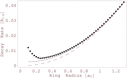
Figure 1: Effect of Aharonov-Bohm on the radiative decay of a quantum ring exciton. The dashed(– –), solid, and dotted( $\cdot$) curves correspond to $\Phi=0\Phi_{0},$ $0.25\Phi_{0},$ and $0.5\Phi_{0},$ respectively. In small radius limit, $F_{nm}^{\ast}$ depends strongly on radius $\rho$, and its influence on the decay rate is evident. The vertical and horizontal units here are $\frac{3\pi}{2k_{0}d}\gamma_{0}$ and ring radius (in units of $a_{0}$), respectively.

The dipole matrix element $\mathbf{\chi}_{\nu nm}$ in Eq. (14) corresponds to an average of dipole transitions between different sites, weighted by the exciton wave function $F_{nm}^{\ast}(\varphi_{e}).$ The sum in Eq. (14) contains a $\varphi_{e}\rightarrow 0$ term in which the electron and the hole are at the same site. If the corresponding integral does not vanish, this term dominates the sum. The effective dipole transition matrix element becomes

$$\mathbf{\chi}_{\nu nm}\sim F_{nm}^{\ast}(0)\int d\mathbf{\varphi}w_{c}^{\ast}(\varphi)(-i\hbar\mathbf{\nabla})w_{v}(\mathbf{\varphi})=F_{nm}^{\ast}(0)\chi_{s},$$ (19)

where $\chi_{s}$ is essentially the dipole matrix element between the atomic states at the same site. Combing Eqs. (13), (15), (17), and (19), one can obtain the AB effect for a superradiant exciton. In Fig. 1 three curves of different flux $\Phi$ are presented as a function of radius $\rho$. To plot the figure, we have assumed the wavelength of the emitted photon $\lambda=8000\overset{\circ}{A}$ and lattice spacing $d=5\overset{\circ}{A}$. The dashed, solid, and dotted curves represent the cases of $\Phi=0\Phi_{0},$ $0.25\Phi_{0},$ and $0.5\Phi_{0},$ respectively. As can be seen, AB effect becomes important in small radius limit. For $\Phi=0.5\Phi_{0}$, the decay rate decreases with the decreasing of ring radius but reaches the minimum point as $\rho$ is about 0.25$a_{0}$ (where $a_{0}=100\overset{\circ}{A}$ is the effective Bohr radius we assumed in 1D limit). This is because the probability, for electron and hole to meet each other on the opposite side of the ring, increases with the decreasing of ring radius, while the coherent effect (superradiance) decreases with the decreasing of the radius. As a result, there is a competition between these two effects. One also notes the AB oscillation is not of constant amplitude. In Fig. 2, relative decay rates [$\gamma_{{}_{\nu nm}}(\Phi)-\gamma_{{}_{\nu nm}}(\Phi=0)$] as a function of magnetic flux $\Phi$ are plotted. The solid and dashed lines represent the cases of $\rho=1$ $a_{0}$ and $\rho=0.5$ $a_{0}$ , respectively. The larger the radius, the smaller the AB oscillation amplitude. As expected, the superradiant decay rate is most enhanced for $\Phi=0.5\Phi_{0}$, and the oscillation period is equal to $\Phi_{0}=hc/e$.

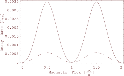
Figure 2: Dependence of relative decay rate [$\gamma_{{}_{\nu nm}}(\Phi)-\gamma_{{}_{\nu nm}}(\Phi=0)$] on the magnetic flux. The dashed and solid curves correspond to $\rho=0.5$ $a_{0}$ and $\rho=1$ $a_{0},$ respectively. The vertical and horizontal units are $\frac{3\pi}{2k_{0}d}\gamma_{0}$ and universal flux quantum $\Phi_{0}=hc/e,$ respectively.

Although present model considers the ideal one-dimensional quantum ring, the physics discussed above can be applied to the realistic quantum ring with finite width. The modified quantity is the exciton wavefunction $F_{nm},$ which only changes the amplitude of AB oscillation. In addition, the coherent radiation from the lattice points within a wavelength still holds as long as the angular momentum is preserved, i.e. not broken by impurities or phonons. This means a high quality quantum is required to observe the mentioned effects.

In summary, we have calculated the superradiant decay rate of an exciton in a quantum ring. Flux dependent oscillation of the superradiant exciton is shown explicitly. With the decreasing of ring radius, there is a competition between the superradiant and AB effects. The distinguishing features are pointed out and may be observed in a suitably designed experiment.

This work is supported partially by the National Science Council, Taiwan under the grant number NSC 92-2120-M-009-010.

References

(1) A. Lorke, R. J. Luyken, A. O. Govorov, J. P. Kotthaus, J. M.
Garcia, and P. M. Petroff, Phys. Rev. Lett. 84, 2223 (2000).
(2) V. Gudmundsson, C. S. Tang, and A. Manolescu, Phys. Rev. B 67, 161301 (2003); A. O. Govorov, S. E. Ulloa, K. Karrai, and R. J.
Warburton, Phys. Rev. B 66, 081309 (2002); O. Voskoboynikov, Yiming
Li, Hsiao-Mei Lu, Cheng-Feng Shih, and C. P. Lee, Phys. Rev. B 66,
155306 (2002); Hui Hu, Guang-Ming Zhang, Jia-Lin Zhu, and Jia-Jiong Xiong,
Phys. Rev. B 63, 045320 (2001).
(3) Y. Gefen, Y. Imry, and M. Y. Azbel, Phys. Rev. Lett. 52, 129 (1984); M. Büttiker, Y. Imry, R. Landauer, and S. Pinhas, Phys.
Rev. B 31, 6207 (1985); Z. S. Ma, K. A. Chao, G. P. He, Solid
State Commun. 122 , 217 (2002).
(4) M. Bayer, M. Korkusinski, P. Hawrylak, T. Gutbrod, M. Michel,
and A. Forchel, Phys. Rev. Lett. 90, 186801 (2003).
(5) J. J. Hopfield, Phys. Rev. 112, 1555 (1958).
(6) V. M. Agranovich and O. A. Dubovskii, JETP Lett. 3, 223
(1966); A. L. Ivanov and H. Haug, Phys. Rev. Lett. 71, 3182 (1993);
Y. N. Chen, D. S. Chuu, T. Brandes, and B. Kramer, Phys. Rev. B 64,
125307 (2001).
(7) K. C. Liu and Y. C. Lee, Physica 102A, 131 (1980); J.
Knoester, Phys. Rev. Lett. 68, 654 (1992); D. S. Citrin, Phys.
Rev. B 47, 3832 (1993); D. Ammerlahn, J. Kuhl, B. Grote, S. W.
Koch, G. Khitrova, and H. Gibbs, Phys. Rev. B 62, 7350 (2000); Y.
N. Chen and D. S. Chuu, Phys. Rev. B 61, 10815 (2000).
(8) E. Hanamura, Phys. Rev. B 38, 1228 (1988); G. Björk
, S. Pau, J. M. Jacobson, H. Cao, and Y. Yamamoto, Phys. Rev. B 52,
17310(1995); Y. N. Chen, D. S. Chuu, and T. Brandes, Phys. Rev. Lett.
90, 166802 (2003).
(9) Y. N. Chen and D. S. Chuu, Physica B 334, 175 (2003).
(10) R. A. Römer and M. E. Raikh, Phys. Rev. B 62, 7045
(2000).