Phase slips in superconducting films with constrictions

Abstract

A system of two coplanar superconducting films seamlessly connected by a bridge is studied. We observe two distinct resistive transitions as the temperature is reduced. The first one, occurring in the films, shows some properties of the Berezinskii-Kosterlitz-Thouless (BKT) transition. The second apparent transition (which is in fact a crossover) is related to freezing out of thermally activated phase slips (TAPS) localized on the bridge. We also propose a powerful indirect experimental method allowing an extraction of the sample’s zero-bias resistance from high-current-bias measurements. Using direct and indirect measurements, we determined the resistance $R(T)$ of the bridges within a range of eleven orders of magnitude. Over such broad range, the resistance follows a simple relation $R(T)=R_{N}\text{ exp }[-(c/t)(1-t)^{3/2}]$, where $c=\Delta F(0)/kT_{c}$ is the normalized free energy of a phase slip at zero temperature, $t=T/T_{c}$ is normalized temperature, and $R_{N}$ is the normal resistance of the bridge.

I Introduction

Thermally activated vortex-like excitations (topological defects) of the superconducting condensate is the primary source of dissipation in mesoscopic superconducting structures.tinkham_text These fluctuations take different forms in one-dimensional (1D) and two-dimensional (2D) systems. In 2D thin films the fluctuations are known to be broken vortex-antivortex pairs berezinskii ; kosterlitz_thouless ; kosterlitz ; beasley_etal ; halperin_nelson ; minnhagen ; bancel_gray ; hebard_fiory ; rosario_etal ; strachan_etal while in 1D wires the resistance is due to phase slips.little ; langer_ambegaokar ; mccumber_halperin ; lukens_etal ; newbower_etal ; sharifi_etal ; lau_etal ; tinkham_lau ; rogachev_bezryadin ; bollinger_etal One important difference between these two types of fluctuations is that vortices and antivortices form bound pairs below a certain critical temperature, known as the Berezinskii-Kosterlitz-Thouless (BKT) transition temperature, while phase slips and anti-phase-slips are unbound at any finite temperature. Thus the resistance of 1D wires is greater than zero at any finite temperature due to the presence of phase slips, which are described by the theory of Langer, Ambegaokar, McCumber, and Halperin (LAMH), langer_ambegaokar ; mccumber_halperin

Here we report a study of structures in which both types of fluctuations can coexist, namely thin films containing constrictions, which are comparable in size to the coherence length. The goals of this work are (i) to test the applicability of the LAMH theory for short and rather wide constrictions and (ii) to test the effect of the vortex-antivortex sea existing in the thin film banks adjacent to the constriction on the phase slippage rate on the constriction itself. For this purpose we fabricate and measure a series of thin superconducting MoGe filmsgraybeal_thesis (which are about 15 $\mu$m wide) interrupted by constrictions or “bridges” (see Fig. 1a). The width of the narrowest point of the bridges is in the range of 13-28 nm, i.e. a few times larger than the coherence length (we estimate $\xi(0)\approx 7$ nm for our MoGe filmsbezryadin_etal ). Two resistive transitions are observed in such samples indicating that vortex-antivortex pair binding-unbinding transition (if any) and thermally activated phase slip processes occur separately. For $T>T_{\text{BKT}}$ the contribution of vortex-antivortex pairs is dominant. On the other hand, below $T_{\text{BKT}}$ the transport properties are determined by the phase slip process on the bridge, which may be regarded as a vortex-antivortex pair breaking assisted by the bridge.

Using direct and indirect techniques we have tracked the sample’s resistance within a range of eleven orders of magnitude. The resulting $R(T)$ curves are compared with the LAMH theory. Regardless of the large width of the bridges and their shortness, the shape of the measured $R(T)$ curves is in perfect agreement with the overall shape of the curves computed using the standard LAMH theory (note that this theory was originally derived for very long wires that are much thinner than the coherence length). The only disagreement found with LAMH is that the pre-exponential factor had to be modified in order to obtain a reasonably low critical temperature of the bridges. (The critical temperature is used as an adjustable parameter in the fitting procedure.) Following the argument of Littlelittle we arrive at the conclusion that the pre-exponential factor should be simply $R_{N}$ and obtain a good agreement with measured curves. The measurements show that the bridges with intermediate dimensions (i) allow phase slippage which does not quench at any finite temperature, (ii) behave independently of the thin film banks, and (iii) exhibit a higher rate of phase slippage in the cases when the width of the bridge is smaller and therefore when the coupling between the thin film banks is weaker.

Before presenting our experimental results we give a brief summary of the BKT theory of topological phase transitions and the LAMH theory of thermally activated phase slips. In thin superconducting films, even in the absence of a magnetic field, an equal population of free vortices and antivortices is expected to occur. The BKT theory predicts a universal jump in the film superfluid density $n_{s}$ at the characteristic temperature $T_{\text{BKT}}$, lower than the mean field critical temperature of the film $T_{c0}$. Such a jump is related to the vortex-antivortex pair binding through a logarithmic interaction potential between free vortices kosterlitz_thouless ; goldman_etal . Applied currents can break bound pairs producing free vortices and leading to non-linear $V(I)$ curves. Above $T_{\text{BKT}}$ the linear resistance of a film is given by the Halperin-Nelson (HN) formulahebard_fiory ; halperin_nelson

$$R_{\text{HN}}=10.8bR_{n,\text{f}}\ \text{exp}\left[-2\sqrt{b(T_{c0}-T_{\text{BKT}})/(T-T_{\text{BKT}})}\right]$$ (1)

where $R_{n,\text{f}}$ is the normal state resistance per square of the film and $b$ is a non-universal constant. Note that the HN equation predicts zero resistance for temperatures below the BKT phase transition temperature $T_{\text{BKT}}$.

The LAMH theorytinkham_text ; little ; langer_ambegaokar ; mccumber_halperin applies to narrow superconducting channels, in which thermal fluctuations can cause phase slips, i.e. jumps by $2\pi$ of the phase difference of the superconducting order parameter. In unbiased samples the number of phase slips (which change the phase difference by $2\pi$) equals the number of anti-phase-slips (which change the phase difference by $-2\pi$). An applied bias current pushes the system away from the equilibrium and the number of phase slips becomes larger than the number of anti-phase-slips. Thus a net voltage appears on the sample, which can be calculated, following LAMH, as $V=\hbar\dot{\phi}/2e$ (below we will also discuss an alternative approach to the voltage definition). Here $\hbar$ is Planck’s constant, $e$ is the electron charge, and $\dot{\phi}$ is the rate of change of the phase difference between the ends of the wire. During the phase slip process the energy of the system increases since the order parameter becomes suppressed to zero in the center of the phase slip. Thermal activations of the system over this free energy barrier $\Delta F(T)$ occur at a rate given by $(\Omega(T)/2\pi)e^{-\Delta F/kT}$. If the bias current is not zero, then the net rate of the phase slippage is $\dot{\phi}=\Omega(T)(e^{-\Delta F_{+}(I)/kT}-e^{-\Delta F_{-}(I)/kT})$. Here $I$ is the bias current, and $\Delta F_{+}$ and $\Delta F_{-}$ are the barriers for phase slips and anti-phase-slips correspondingly (these two barriers become equal to each other at zero bias current). The attempt frequency derived from a time-dependent Ginzburg-Landau (GL) theory, for the case of a long and thin wire, ismccumber_halperin

$$\Omega(T)=\frac{L}{\xi(T)}\frac{1}{\tau_{\text{GL}}}\left(\frac{\Delta F}{kT}\right)^{1/2}$$ (2)

where $T$ is the temperature of the wire, and $L/\xi(T)$ is the length of the wire measured in units of the GL coherence length $\xi(T)$. The attempt frequency is inversely proportional to the relaxation time $\tau_{\text{GL}}=\pi\hbar/8k(T_{c}-T)$ of the time-dependent GL theory, with $T_{c}$ being the mean field critical temperature of the wire (or of the bridge, as in our discussions below). The factor $\left(\Delta F/kT\right)^{1/2}$ provides a correction for the overlap of fluctuations at different places of the wire and the factor $L/\xi(T)$ gives the number of statistically independent regions in the wiremccumber_halperin . The free energy barrier for a single phase slip is given langer_ambegaokar ; tinkham_lau by

$$\Delta F=\frac{8\sqrt{2}}{3}\frac{H_{c}^{2}(T)}{8\pi}A\xi(T),$$ (3)

which is essentially the condensation energy density $H_{c}^{2}(T)/8\pi$ multiplied by the effective volume $8\sqrt{2}A\xi(T)/3$ of a phase slip ($A$ is the cross-section area of the wire).

A bias current $I$ causes a non-zero voltage (time averaged) given by

$$V=\frac{\hbar\Omega(T)}{e}e^{-\Delta F/kT}\sinh(I/I_{0})$$ (4)

where $I_{0}=4ekT/h$ ($I_{0}=13.3$ nA at $T=1$ K). Differentiation of this expression with respect to the bias current $I$ gives the differential resistance

$$dV/dI=\frac{\hbar\Omega(T)}{eI_{0}}e^{-\Delta F/kT}\cosh(I/I_{0})$$ (5)

The dependence of the attempt frequency and free energy on the bias current is neglected in this derivation. In the limit of low currents $I\ll I_{0}$, Ohm’s law is recovered

$$R_{\text{LAMH}}(T)=\frac{\hbar\Omega(T)}{eI_{0}}e^{-\Delta F/kT}=R_{q}\left(\frac{\hbar\Omega(T)}{kT}\right)e^{-\Delta F/kT}$$ (6)

where $R_{q}=h/(2e)^{2}=6.5$ k$\Omega$. In this approach the fluctuation resistance does not have any explicit dependence on the normal resistance of the wire.

II Experimental Setup

The sample geometry is shown schematically in Fig. 1a. The fabrication is performed starting with a Si wafer covered with SiO₂ and SiN films. A suspended SiN bridge is formed using electron beam lithography, reactive ion etching, and HF wet etching.bezryadinJVST The bridge and the entire substrate are then sputter-coated with amorphous Mo₇₉Ge₂₁ superconducting alloy, topped with a $2$ nm overlayer of Si for protectionsputter . The resulting bridges are $100$ nm long with a minimum width $w\approx$ 13-28 nm as measured with a scanning electron microscope (SEM) (Fig. 1b). All samples are listed in Table I.

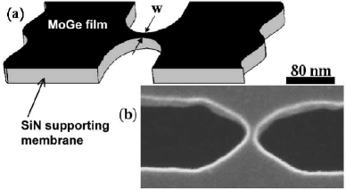
Figure 1: (a) Sample schematic. MoGe film (black) of thickness $d=$ 2.5–4.5 nm is deposited over a SiN membrane (gray) substrate with a constriction of width $w$. (b) An SEM micrograph of a typical sample. The MoGe coated SiN bridge (gray) is suspended over a deep trench (black).

Transport measurements are performed in a pumped ⁴He cryostat equipped with a set of rf-filtered leads. The linear resistance $R(T)$ is determined from the low-bias slope (the bias current is in the range of 1-10 nA) of the voltage versus current curves. The high-bias differential resistance is measured using an ac excitation on top of a dc current offset generated by a low-distortion function generator (SRS-DS360) connected in series with a 1 M$\Omega$ resistor. One sample was measured down to the m$\Omega$ level using a low temperature transformer manufactured by Cambridge Magnetic Refrigeration.

Sample	$w$ (nm)	$R_{N}$ ($\Omega$)	$T_{c}$ (K)	$T_{c0}$ (K)	$d$ (nm)	$\beta$
A1	$27\pm 4$	$1380$	$3.88$	$3.90$	$2.5$	$1.47$
B1	$13\pm 4$	$1650$	$4.80$	$4.91$	$3.5$	$0.723$
B2	$28\pm 4$	$1320$	$4.81$	$4.91$	$3.5$	$1.10$
C1	$13\pm 4$	$1440$	$5.16$	$5.50$	$4.5$	$0.653$
C2	$27\pm 4$	$680$	$5.39$	$5.50$	$4.5$	$2.21$

Table 1: Sample parameters, including the width of the constriction ($w$), determined from SEM images, normal resistance of the bridge ($R_{N}$), determined from the $R(T)$ curves (at a temperature slightly below the resistive transition of the thin film banks), critical temperature ($T_{c}$), determined from $R_{\text{WL}}(T)$ fits given by Eq. (9)), critical temperature of the film ($T_{c0}$), film thickness ($d$), and a geometrical fitting parameter ($\beta$).

III Results

First we compare a sample with a hyperbolic constriction (“bridge sample”) with a reference sample, which is a plain MoGe film of the same thickness, without any constriction (“film sample”). Both are fabricated on the same substrate simultaneously. A resistive transition measured on the film sample is shown in Fig. 2. The HN fit generated by Eq. (1) is shown as a solid line and exhibits a good agreement with the data, yielding a BKT transition temperature of $T_{\text{BKT}}=4.8$ K and the mean field critical temperature $T_{c0}=4.91$ K. Such good fit suggests that the transition observed in the banks might be the BKT transition, although a more extensive set of experiments is necessary in order to prove this assumption rigorously. As expected, $T_{\text{BKT}}$ is slightly lower than $T_{c0}$. The inset of Fig. 2 compares the $R(T)$ measurements of the “film” (open circles) and the “bridge” (solid line) samples. At $T=4.8$ K the $R(T)$ curve for the film sample crosses the $R=0$ axis with a nonzero (and large) slope, in agreement with the behavior predicted by the HN resistance equation (1). Nevertheless, unlike the film sample, the bridge sample shows a non-zero resistance even below the BKT transition temperature predicted by Eq. (1). Such resistive tails, occurring at $T<T_{\text{BKT}}$, have been found in all samples with constrictions.

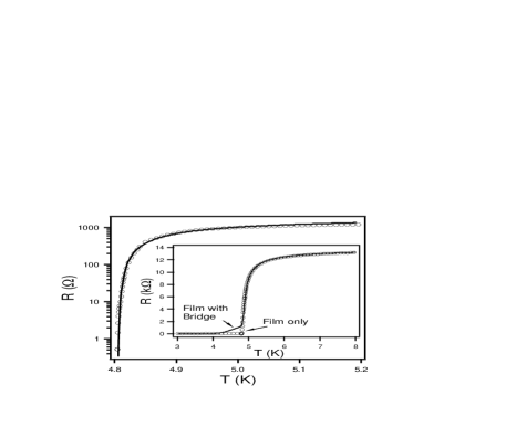
Figure 2: Low-bias resistance versus temperature dependence (open circles), measured on a thin film ($d=3.5$ nm) without constriction. The solid line is a fit to the Halperin-Nelson theory (Eq. (1)). (Inset): Resistance of the film without constriction (multiplied by a constant factor), shown as open circles, is compared to the sample with a hyperbolic bridge (B2), shown by the solid line. The only qualitative difference is the presence of a “resistive tail”, observed on all samples with constrictions.

In Fig. 3 the $R(T)$ curves for five samples with bridges are plotted in a log-linear format. The resistance of sample B1 has been measured down to the m$\Omega$ range using a low temperature transformer. Two resistive transitions are seen in each curve as the temperature decreases. The first transition is the superconducting transition in the thin film banks adjacent to the bridge. The second transition corresponds to the resistive tail mentioned above. In order to understand the origin of the second transition it should be compared to the LAMH theory.

IV Discussion

Below we analyze the resistive tails found on samples with constrictions and demonstrate that they are caused by the phase slip events localized on the bridges and behave independently of the adjacent thin film banks. The analysis indicates that no BKT (no vortex-antivortex binding within the constrictions) or any other type of transition occurs on the constrictions and that the phase slips and anti-phase-slips are unpaired at any nonzero temperature due to thermal fluctuations. This is demonstrated below by fitting the $R(T)$ curves with the LAMH-like fitting curves.

IV.1 LAMH attempt frequency for a short bridge

In order to compare our results to the LAMH we have to take into account the small length of the bridge, which does not allow more than one phase slip at a give time. Therefore the attempt frequency $\Omega(T)$ of Eq. (2) can be simplified. First, it has a term $L/\xi(T)$ that accounts for the number of independent sites where a phase slip can occur mccumber_halperin . Since each of our samples has only one narrow region where phase slip events can happen, we take $L/\xi(T)=1$. Second, the coefficient $(\Delta F/kT)^{1/2}$ which takes into account possible overlaps of phase slips at different places along the wiremccumber_halperin is taken to be unity also. This is because for short hyperbolic bridges (not much longer than the coherence length) it is reasonable to expect that there is only one spot, i.e. the narrowest point of the bridge, where phase slips occur. As a result, we obtain the attempt frequency for a short hyperbolic bridge $\Omega_{\text{WL}}=1/\tau_{\text{GL}}$ (the abbreviation “WL” stands for “weak link”). This attempt frequency can be combined with the usual form of the LAMH resistance in Eq. (6) and can be used to fit the experimental $R(T)$ curves (below the resistive transition of the films). Although such fits follow the data very well, there is one inconsistency that is they require the critical temperature of the bridge to be chosen higher than the critical temperature of the films, which is unphysical for such system. We attempt to modify the pre-exponential factor in order to resolve this inconsistency, as discussed below.

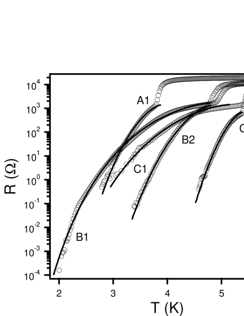
Figure 3: Low-bias resistance for five different samples with bridges. The parameters of the samples are given in Table 1. The data points are shown by open symbols. Solid lines are fits to the “bridge” phase slip model given by Eqs. (7) and (9).

IV.2 Modification of the prefactor

Since the exact expression is unknown, we approximate the resistance of a constriction (weak link) as

$$R_{\text{WL}}(T)=R_{N}\ e^{-\Delta F_{\text{WL}}/kT}.$$ (7)

The exponential factor here is that of the LAMH theory and the prefactor is simply the normal resistance of the bridge. This expression (Eq. (7)) can be justified by the following argument: the duration of a single phase slip (i.e. the time it takes for the order parameter to recover) is $\sim\tau_{\text{GL}}$ and the number of phase slips occurring per second is $\sim\Omega_{\text{WL}}(T)\ \text{exp}\left[-\Delta F(T)/kT\right]$, with the attempt frequency being the inverse GL relaxation time $\Omega_{\text{WL}}=1/\tau_{\text{GL}}$, as was argued above. Therefore the time fraction during which the constriction is experiencing a phase slip (i.e. when superconductivity is suppressed on the bridge) is the product of these two values, i.e. $f=(\tau_{\text{GL}})(1/\tau_{\text{GL}})\ \text{exp}\left[-\Delta F(T)/kT\right]=\text{exp}\left[-\Delta F(T)/kT\right]$. Following Little,little it can be assumed that the bridge has the normal resistance $R_{N}$ during the time when a phase slip is present (i.e. when the bridge is in the normal state), and the resistance is zero otherwise (when there is no phase slip). Thus we arrive at the averaged resistance for a bridge or a small size weak link $R_{WL}=f\times R_{N}+(1-f)\times 0=R_{N}\ \text{exp}\left[-\Delta F/kT\right]$ as in Eq. (7). Note that unlike in the LAMH theory, in the present formulation the fluctuation resistance is directly linked to to the normal state resistance of the sample.

In order to compare Eq. (7) to the experimental results, an explicit expression for the energy barrier $\Delta F_{\text{WL}}$ for a phase slip localized on the bridge is required. Starting with the usual formtinkham_lau derived for a long 1D wire and some well known results from BCS and GL theory,tinkham_text ; tinkham_lau we find that $\Delta F_{\text{WL}}(0)=(8\sqrt{2}/3)(H_{c}^{2}(0)/8\pi)A\xi(0)=0.83kT_{c}R_{q}L/R_{N}\xi(0)$ where $L$ is the length of the wire. Using $R_{N}=\rho_{n}L/A$, the free energy barrier for a weak link is

$$\Delta F_{\text{WL}}(0)=0.83kT_{c}\frac{\beta wdR_{q}}{\rho_{n}\xi(0)}$$ (8)

where $w$ is the width of the bridge, $d$ is the film thickness, $\rho_{n}$ is the normal resistivity, and $A=wd$. The parameter $\beta$ measures the ratio of the phase slip length along the bridge to the effective length of a phase slip in a 1D wire, which is equal to $8\sqrt{2}\xi(T)/3$. Finally, assuming the same temperature dependence of the barrier as in the LAMH theory, i.e. $\Delta F(T)=\Delta F(0)(1-T/T_{c})^{3/2}$, we arrive at the expression for the bridge fluctuation-induced resistance:

$$R_{\text{WL}}(T)=R_{N}\ \text{exp}\left[-0.83\frac{\beta wdR_{q}}{\rho_{n}\xi(0)}\left(1-\frac{T}{T_{c}}\right)^{3/2}\frac{T_{c}}{T}\right].$$ (9)

The fits generated by Eq. (9) are shown in Fig. 3 as solid lines. An impressively good agreement is found for all five samples. In particular, sample B1 measured using the low-temperature transformer, shows an agreement with the predicted resistance $R_{\text{WL}}$ over about seven orders of magnitude, down to a temperature that is more than two times lower compared to the critical temperature of the sample. Only two fitting parameters are used: $\beta$ and $T_{c}$ (listed in Table 1). The other parameters required in Eq. (9), including $R_{N}$, $d$, $w$, $\xi(0)$, and $\rho_{n}\approx 180$ $\mu\Omega$ cm are known.bezryadin_etal ; tinkham_lau ; lau_etal The fits give quite reasonable values for the critical temperature of the bridges, in the sense that they are slightly lower than the corresponding critical temperatures of thin films of the same thickness, as expected. This fact supports the validity of Eq. (7). Such good agreement also indicates that the dissipation in a thin film with a constriction at $T<T_{\text{BKT}}$ is solely due to thermal activation of phase slips on constrictions. As expected, $\beta\approx 1$ for all samples and the larger $\beta$ values are found on wider constrictions.

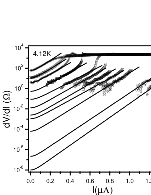
Figure 4: Differential resistance as a function of the dc bias current for sample B2. Experimental data are denoted by open symbols and the solid lines are fits to $dV/dI=R(T)\cosh(I/I_{0})$. Temperatures from left to right are $4.12$, $3.92$, $3.80$, $3.64$, $3.45$, $3.36$, $3.26$, $3.16$, $3.07$, $2.80$ and $2.68$ K.

IV.3 Determination of the linear resistance from high bias current measurements

We now discuss the non-linear properties of films with constrictions. Measurements of the differential resistance versus bias current, $dV/dI$ vs. $I$, are plotted in Fig. 4 on log-linear scale. Using these results it is possible to distinguish between the BKT mechanism, which leads to a power-law $V(I)$ dependence, and the phase slippage process, which is characterized by an exponential $V(I)$ dependence (Eqs. (4) and (5)). From Fig. 4 it is clear that at $T<T_{\text{BKT}}$ and sufficiently low currents the dependence of the differential resistance on bias current is exponential (it appears linear on the log-linear plots). Thus it is appropriate to compare the results with the LAMH theory. Equation (5) can be written as $dV/dI=R(T)\cosh(I/I_{0})$, where $R(T)$ is the temperature-dependent zero-bias resistance. Using this relation, we fit the differential resistance data and use $R(T)$ as a fitting parameter, as shown in Fig. 4 by solid lines, each corresponding to a fixed temperature.i0 The fitting procedure illustrated in Fig. 4 gives us a powerful indirect method of determination of the zero-bias resistance (it is implicitly assumed that the ratio of the rates of thermally activated and quantum phase slips (if any) is independent of the bias current). This method is useful when the temperature is low and the resistance of the sample is below the resolution limit of the experimental setup. Thus, by fitting the $dV(I)/dI$ curves, we obtained the zero-bias resistance $R(T)$ down to very low values ($\sim 10^{-8}$ $\Omega$). This method was systematically applied on sample B2 and the results are shown in Fig. 5 as solid squares. The open circles in Fig. 5 represent the zero-bias resistance obtained by direct measurements at low bias currents. The two sets of data are consistent with each other. The solid curve in Fig. 5 is a $R_{\text{WL}}$ fit obtained using Eq. (9). An excellent agreement is seen in a wide range of resistances spanning eleven orders of magnitude. This re-confirms that the thermally activated phase slip mechanism is dominant in the bridge samplesnanowire_also for $T<T_{\text{BKT}}$. We emphasize that the critical temperature of the bridge, which is used as an adjustable parameter, is found to be $T_{c}=4.81$ K. As expected, the $T_{c}$ of the bridge is slightly lower than the critical temperature of the film electrodes $T_{c0}=4.91$ K.

Figure 5: Resistance vs. temperature curve for sample B2. Open circles represent data that have been directly measured while filled boxes give the resistance values determined by fitting the $dV/dI$ curves of Fig. 4 using the formula $dV/dI=R(T)\cosh(I/I_{0})$. The solid and the dashed curves give the best fits generated by the $R_{\text{WL}}(T)$ ($T_{c}=4.81$ K) and $R_{\text{LAMH}}(T)$ ($T_{c}=5.38$ K) formulas, respectively.

The usual LAMH expression $R_{\text{LAMH}}$ (Eq. (6)), which applies to thin superconducting wires, tinkham_lau ; lau_etal ; rogachev_bezryadin ; bezryadin_etal can also be used to fit our data. The overall shape of the fitting curve (dashed curve in Fig. 5) agrees with the data as well as with the $R_{\text{WL}}$ fit. The drawback of the usual LAMH formula is that the critical temperature of the bridge, which is used as an adjustable parameter, turns out considerably higher than the film transition temperature. For example, the dashed line fit in Fig. 5 is generated using $T_{c}=5.38$ K which is larger than the film critical temperature $T_{c0}=4.91$ K. This apparent enhancement of the critical temperature of the bridge must be an artifact, because a reduction of the dimensions of MoGe samples always leads to a reduction of the critical temperature.Oreg On the other hand, the $T_{c}$ extracted from the fits made using Eq. (9) are almost equal and slightly lower than the film $T_{c0}$ (Table I), as expected.

A rapid decrease of the LAMH resistance at temperatures very close to the critical temperature reflects the behavior of the LAMH attempt frequency which approaches zero as $T\rightarrow T_{c}$. The LAMH resistance is proportional to the attempt frequency so we observe $R\rightarrow 0$ as $T\rightarrow T_{c}$ (dashed curve in Fig. 5 ). Such behavior is unphysical and occurs since the LAMH theory is not applicable very near $T_{c}$. It should be emphasized that some of our measured bridges are wider than $\xi(0)$, yet the thermally activated phase slip model agrees well with the data. This is in agreement with the prediction (Ref. langer_ambegaokar, , p. 510) that superconducting channels of width $w\lesssim 4.4\xi(T)$ should exhibit a 1D behavior, i.e. nucleation of vortices is unfavorable in such channels. Such condition is true for all of our samples.

V Summary

Fluctuation effects in thin films interrupted by “hyperbolic” constrictions is studied. The measurements show two separate resistive transitions. The higher-temperature transition shows some properties of a BKT transition in the films (follows the HN formulae). The second apparent resistive transition is explained by a continuous reduction of the rate of thermally activated phase slips with decreasing temperature. A quantitative description of the fluctuation resistance of narrow and short superconducting constrictions is achieved. For this purpose we have modify the LAMH expression for the resistance of a one-dimensional nanowire. An indirect method that enables us to trace the resistance variation over eleven orders of magnitude is suggested, based on the analysis of the nonlinear effects occurring at high bias currents. The phase slippage model is found applicable in the entire range of measured resistances, suggesting that quantum phase slipslau_etal do not occur in this samples, in the studied temperature interval, which extends below $T_{c}/2$ for one sample (B1)).

- (1) M. Tinkham, Introduction to Superconductivity (McGraw Hill, New York, 1996).
- (2) V.L. Berezinskii, Zh. Exp. Theor. Fiz. 59, 907 (1970) [Sov. Phys. JETP. 32, 493 (1971)]
- (3) J.M. Kosterlitz and D.J. Thouless, J. Phys. C 6, 1181 (1973).
- (4) J.M. Kosterlitz, J. Phys. C 7, 1046 (1974).
- (5) M.R. Beasley, J.E. Mooij, and T.P. Orlando, Phys. Rev. Lett. 42, 1165 (1979).
- (6) B.I. Halperin and D.R. Nelson, J. Low Temp. Phys. 36, 599 (1979).
- (7) P. Minnhage, Rev. of Mod. Phys. 59, 1001 (1987).
- (8) P.A. Bancel and K.E. Gray, Phys. Rev. Lett. 46, 148 (1981).
- (9) A.F. Hebard and A.T. Fiory, Phys. Rev. Lett. 50, 1603 (1983).
- (10) M.M. Rosario, Yu. Zadorozhny, and Y. Liu, Phys. Rev. B 61, 7005 (2000).
- (11) D.R. Strachan, C.J. Lobb, and R.S. Newrock, Phys. Rev. B 67, 174517 (2003).
- (12) W.A. Little, Phys. Rev. 156, 396 (1967).
- (13) J.S. Langer and V. Ambegaokar, Phys. Rev. 164, 498 (1967).
- (14) D.E. McCumber and B.I. Halperin, Phys. Rev. B 1, 1054 (1970).
- (15) J.E. Lukens and R.J. Warburton, and W.W. Webb, Phys. Rev. Lett. 25, 1180 (1970).
- (16) R.S. Newbower, M.R. Beasley, and M. Tinkham, Phys. Rev. B5, 864 (1972).
- (17) F. Sharifi, A.V. Herzog, and R.C. Dynes, Phys. Rev. Lett. 71, 428 (1993).
- (18) M. Tinkham and C.N. Lau, Appl. Phys. Lett. 80, 2946 (2002).
- (19) C.N. Lau, N. Markovic, M. Bockrath, A. Bezryadin, and M. Tinkham, Phys. Rev. Lett. 87, 217003 (2001).
- (20) A. Rogachev and A. Bezryadin, Appl. Phys. Lett. 83, 512 (2003).
- (21) A.T. Bollinger, A. Rogachev, M. Remeika, and A. Bezryadin, Phys. Rev. B 69, R180503 (2004).
- (22) J.M. Graybeal and M.R. Beasley, Phys. Rev. B29, 4167 (1984); J.M. Graybeal, Ph.D. thesis, Stanford University, 1985.
- (23) A. Bezryadin, C.N. Lau, and M. Tinkham, Nature 404, 971 (1999).
- (24) A. Bezryadin and C. Dekker, J. Vac. Sci. Technol. B 15, 793 (1997).
- (25) MoGe was dc sputtered while Si was rf sputtered. The sputtering system was equipped with a liquid-nitrogen-filled cold trap and had a base pressure of Torr.
- (26) A.M. Kadin, K. Epstein, and A.M. Goldman, Phys. Rev. B 27, 6691 (1983).
- (27) The parameter was also used as a fitting parameter in order to obtain the best fitting results. Some deviations of this parameter from the theoretical value can be explained by the Joule heating of the bridges, which may become significant high bias currents.
- (28) Y. Oreg and M. Finkel’stein, Phys. Rev. Lett. 83, 191 (1999).
- (29) This same method of resistance determination from high bias differential resistance measurements were applied to superconducting Mo79Ge21 nanowires templated by nanotubes (see Refs. lau_etal, ; rogachev_bezryadin, ; bollinger_etal, ; bezryadin_etal, regarding general information about the sample fabrication) and found to also work over a resistance range of twelve orders of magnitude. This data is to be published elsewhere.