Superconducting fluctuation corrections to ultrasound attenuation in layered superconductors

Abstract

We consider the temperature dependence of the sound attenuation and sound velocity in layered impure metals due to $s$-wave superconducting fluctuations of the order parameter above the critical temperature. We obtain the dependence on material properties of these fluctuation corrections in the hydrodynamic limit, where the electron mean free path $\ell$ is much smaller than the wavelength of sound and where the electron collision rate $\tau^{-1}$ is much larger than the sound frequency. For longitudinal sound propagating perpendicular to the layers, the open Fermi surface condition leads to a suppression of the divergent contributions to leading order, in contrast with the case of paraconductivity. The leading temperature dependent corrections, given by the Aslamazov-Larkin, Maki-Thompson and density of states terms, remain finite as $T\rightarrow T_{c}$. Nevertheless, the sensitivity of new ultrasonic experiments on layered organic conductors should make these fluctuations effects measurable.

The problem of fluctuations of the superconducting order parameter above the critical temperature began to attract the attention of researchers more than three decades ago. AL ; Maki ; Thompson Considerable work has been done from both the theoretical and experimental points of view. Conductivity, thermoconductivity, magnetoconductivity as well as tunneling properties and nuclear magnetic resonance characteristics are amongst the various transport phenomena where fluctuation contributions were predicted and experimentally observed. Ref. LV01 contains an extensive review of the field and references.

In the present paper, we concentrate on the superconducting fluctuation corrections to the sound velocity and sound attenuation in layered superconductors above $T_{c}$. As usual, superconducting fluctuations manifest themselves in three different ways. LV01 a) The effective number of normal carriers is reduced because some of the electrons exist as transient Cooper pairs. This is the so-called density of states contribution. b) The single-particle excitations are Andreev reflected off the superconducting fluctuations, as described by the so-called Maki-Thompson term. c) Some of the electrons behave like Cooper pairs for a time given by the Ginzburg-Landau time. This is the famous Aslamazov-Larkin contribution. Layered organic superconductors, in particular, are an ideal class of materials to study fluctuation phenomena. This is because the relatively low charge-carrier concentration and the strong electronic anisotropy enhance the effect of superconducting fluctuations and increase the size of the fluctuation regime. The manifestation of superconducting fluctuations in organic materials was found in a number of experimental works on dc-magnetoconductivity, thermoconductivity, ac-susceptibility, specific heat and torque magnetometry. fluct_ex Preliminary ultrasonic experiments in the $\kappa$-phase layered organic materials usherb (BEDT-TTF)₂Cu[N(CN)₂]Br, (BEDT-TTF)₂Cu[N(CN)₂]Cl and (BEDT-TTF)₂Cu(NCS)₂ suggest that the sound attenuation coefficient is decreased by superconducting fluctuations over a sizeable temperature range above $T_{c}$. However, the effect is much weaker than the fluctuation correction to the conductivity KFrikash where, in the same compounds, the Aslamazov-Larkin contribution dominates the superconducting fluctuation effects. Although sound attenuation experiments seem to be a very promising method to study fluctuation phenomena in layered superconductors, the theoretical description is still incomplete and needs to be analyzed in more details. This more detailed analysis can tell us, for example, which material properties control fluctuation phenomena. Fluctuation phenomena can then be used to access these properties when they are not independently known. For example, we will see that the phase breaking time can be very important to determine the fluctuation contribution to ultrasonic attenuation whereas it would not contribute to dominant terms in the corresponding fluctuation conductivity. It is by considering a large set of experimental probes that one can make sure that all material properties are unambiguously determined.

In this paper we assume, as usual for fluctuation corrections, that we are close enough to $T_{c}$ that the characteristic pair frequency is less than temperature (in dimensionless units). This is the so-called renormalized-classical regime. We study the case where longitudinal sound propagates perpendicular to the layers. This is the most relevant case to study since it is most easily accessible experimentally. KFrikash We also consider the hydrodynamic limit where the electron mean free path $\ell$ is much smaller than the wavelength of sound and where the electron collision rate $\tau^{-1}$ is much larger than the sound frequency. In quasi two-dimensional systems, the Fermi surface is opened in the direction perpendicular to the layers. The coupling to the sound comes from the modulation of the hopping integral across the layers, taking also into account the electroneutrality condition in the moving frame. SamokhinWalker The Fröhlich model where phonons couple to the electronic density is not valid.  The most dramatic consequence of the open Fermi surface in such a situation is the suppression of the divergence in the Aslamazov-Larkin and Maki-Thompson terms that often give, by contrast, the most important contribution to the fluctuation correction to the electrical conductivity. Hence, sound propagation is less strongly modified by superconducting fluctuations than the electrical conductivity. All the calculations are performed for $s-$wave superconducting fluctuations. The $d-$wave case needs a separate treatment. d-wave ; Sauls_tau

In the following section, we discuss earlier work and present the Hamiltonian. The diagrams that enter the calculation and then details of the calculation appear in the following sections. The results are gathered in Sec. V and discussed in Sec.VI. The appendix contains mathematical details on the analytic continuation of digamma functions.

I The model and definitions

Ultrasonic attenuation in impure metals was analyzed by Pippard Pippard , using the Boltzmann equation method, and by Tsuneto Tsuneto with the density matrix formalism. Later on, Schmid Schmid , using Green function methods, derived the effective electron-phonon interaction in the presence of impurities taking into account the screening of Coulomb repulsion between electrons. A key point of the approach of Tsuneto, Pippard and Schmid was to consider the electron system in a reference frame moving together with the ion lattice. In an impure metal, the elastic scattering of electrons as well as perfect screening at small phonon momentum and relaxation to equilibrium occur in this oscillating frame. In this formalism, the electron-phonon coupling appears through the stress tensor instead of through the density operator occurring in the Fröhlich model. The latter model leads to erroneous results in the dirty limit. Schmid

The idea of a moving reference frame was also used by Kotliar and Ramakrishnan Kotliar , who considered the limit of strongly disordered metal and analyzed the effect on ultrasound propagation of incipient localization near the metal-insulator transition. Reizer Reizer considered the effect of various types of inelastic scattering (including electron-electron, electron-magnon scattering and weak-localization effects) on sound attenuation.

The fluctuation corrections to the ultrasound attenuation in 3D metals were estimated in the most singular channel in the early work of Aslamazov and Larkin. AL Aslamazov and Varlamov, back in 1979, found the fluctuation corrections in layered superconductors. AV However, these papers did not consider explicitly the form of the density of states for a corrugated cylindrical Fermi surface. That density of states is energy independent contrary to the assumption made in these papers. In addition, the calculation was done for the Fröhlich model. Also, Ref. AV used impurity vertex corrections for the external vertices in the correlators and we shall see that these are unnecessary in the hydrodynamic limit when one takes into account the fact that the calculation of impurity scattering should be done in the electrically neutral moving frame. Schmid ; Kotliar For the case of interest, with open Fermi surface in the perpendicular direction, we find results that are quite different from these earlier works.

We use the unperturbed quasiparticle energy spectrum

$$\xi(p_{||},p_{z})=\frac{p_{||}^{2}-p_{F}^{2}}{2m}+2t_{\perp}\cos{(p_{z}a)},$$ (1)

appropriate for layered metals. Here, $p_{z}$ is the component of the quasiparticle momentum perpendicular to the conducting planes, $p_{||}$ is the in-plane momentum, $t_{\perp}\ll\varepsilon_{F}$ is the small interlayer hopping energy, and $a$ is the interlayer distance. In this model, the Fermi surface has the well-known shape of a corrugated cylinder, and the density of states is given by $\nu_{0}=m/(2\pi a)$. It is important to note that in this model the density of states $\nu_{0}$ does not depend on the quasiparticle energy. In other words, the derivative $(\partial\nu_{0}/\partial\xi)\equiv 0$ vanishes. This relation is obviously true at $t_{\perp}=0$, i.e. for non-interacting two-dimensional layers. If there is a small interlayer interaction $t_{\perp}\neq 0$, any cross-section of the Fermi surface made at any value of $p_{z}$ still gives the two-dimensional (2D) result with $(\partial\nu_{0}/\partial\xi)\equiv 0$. One can easily see that this relation is valid for any Fermi surface that is opened in the third direction ($t_{\perp}\ll\varepsilon_{F}$) and has circular cross section in the plane.

As shown by Tsuneto Tsuneto and Schmid Schmid , based on earlier work of Pippard Pippard and Blount, Blount the canonical transformation that takes us to the moving frame leads, in the continuum limit, to an electron-phonon interaction that originates from the commutator of the infinitesimal generator of the transformation with the kinetic energy operator. The remaining contributions from the commutator of the generator of the canonical transformation with the electron-ion and electron-electron interactions are overall negligible. Since a trace over fermions is performed to compute phonon damping, the result should be independent of the canonical transformation. The moving frame is the one best suited for approximations.

For a tight binding model, such as the one we need to consider to obtain the proper open Fermi surface for propagation in the perpendicular direction $p_{z}$, Eq. (1), the corresponding microscopic derivation of the stress tensor has not been performed yet. It is not our purpose to give this derivation here. Instead, we follow the footsteps of Barisic, Barisic Su-Schrieffer-Heeger, SuSchrieffer and, more recently, Walker, Smith, and Samokhin SamokhinWalker and assume that the electron-phonon interaction comes from the modulation of the hopping parameter $t_{\perp}$ induced by the lattice deformation. Neglecting umklapp processes, one obtains for the interaction of a longitudinal phonon propagating in the $z$ direction perpendicular to the planes

$$H_{e-ph}=-\sqrt{2}iG\sum_{\mathbf{k,p}}\left(\frac{\hbar\omega_{0}\left(\mathbf{k}\right)}{NMv_{s}^{2}}\right)^{1/2}\left(\widehat{\mathbf{k}}\mathbf{\cdot}\widehat{\mathbf{z}}\right)\left(\widehat{\mathbf{e}}\mathbf{\cdot}\widehat{\mathbf{z}}\right)\left(\cos p_{z}a\right)\text{ }c_{\mathbf{p}+\mathbf{k},\sigma}^{\dagger}c_{\mathbf{p,}\sigma}\left(a_{-\mathbf{k}}^{\dagger}+a_{\mathbf{k}}\right),$$ (2)

where $\omega_{0}\left(\mathbf{k}\right)=v_{s}k$ is the sound frequency, $v_{s}$ the sound velocity, $M$ the ion mass, $N$ the number of unit cells, $G$ a constant that depends on the derivative of the hopping integral $t_{\perp}$ with respect to the strain, while $a_{\mathbf{k}}^{\left(\dagger\right)},c_{\mathbf{p},\sigma}^{\left(\dagger\right)}$ are, respectively, destruction and creation operators for phonons and for electrons of spin $\sigma$. The above expression is restricted to longitudinal phonons propagating in the perpendicular direction, hence the wave vector and polarization of the phonons involved in the interaction will satisfy $\widehat{\mathbf{k}}\mathbf{\cdot}\widehat{\mathbf{z}}=\widehat{\mathbf{e}}\mathbf{\cdot}\widehat{\mathbf{z}}=1$. The above expression neglects the compression and stretching of chemical bonds that are not strictly along the direction of propagation.

II Sound attenuation without fluctuation correction

The sound attenuation coefficient is determined by the imaginary part $\gamma(k)$ of the complex frequency $\omega(k)$ where the pole of the phonon Green function $D(\mathbf{k},\omega)$ is located. This quantity obeys Dyson’s equation AGD

$$D^{-1}(\mathbf{k},\omega_{\nu})=\left(D^{0}(\mathbf{k},\omega_{\nu})\right)^{-1}-\Pi(\mathbf{k},\omega_{\nu}).$$ (3)

Expressed in bosonic Matsubara frequencies $\omega_{\nu}=2\pi\nu T$ using units $k_{B}=1$ $\hbar=1$, with $\nu$ an integer, the quantity $D^{0}(\mathbf{k},\omega_{\nu})$

$$D^{0}(\mathbf{k},\omega_{\nu})=-\frac{\omega_{0}^{2}(\mathbf{k})}{\omega_{\nu}^{2}+\omega_{0}^{2}(\mathbf{k})}$$ (4)

is the phonon propagator in the non-interacting case and $\Pi(\mathbf{k},\omega_{\nu})$ is the phonon self-energy. In an impure metal, the diagrammatic representation of $\Pi(\mathbf{k},\omega_{\nu})$ is given by Fig. 1. In the theory of electronic conductivity, one would consider a similar diagram for the current-current correlator with the bold dots representing the components of the vector velocity $ev_{\alpha}=e(\partial\xi/\partial p_{\alpha})$, where $\xi$ is the electronic energy and $p_{\alpha}$ the $\alpha$ component of momentum. In the case of sound attenuation, the vertex comes instead from the stress tensor corresponding to the electron-phonon interaction Eq. (2). Using Eqs. (2) and (4), one obtains for this vertex $g\cos(p_{z}a)$ where $g$ is a constant.

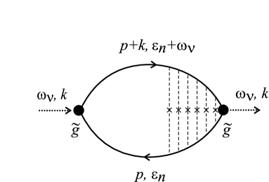
Figure 1: The phonon self-energy in the case of an impure metal. Solid lines are one-electron Green functions, dotted lines the bare phonon propagators, dashed lines with crosses correspond to the impurity scattering, and bold circles show the renormalized electron-phonon vertices.

Each solid line in Fig. 1 corresponds to the electron Green function which, at finite temperature in the presence of impurities, is given by

$$G(\mathbf{p},\varepsilon_{n})=\frac{1}{i\tilde{\varepsilon}_{n}-\xi(\mathbf{p})},$$ (5)

where $\xi(\mathbf{p})$ is the quasiparticle energy and where we defined $\tilde{\varepsilon}_{n}=\varepsilon_{n}+1/(2\tau)\mathrm{sign}(\varepsilon_{n})$ with $\varepsilon_{n}=\pi T(2n+1)$ the Matsubara frequency and $\tau$ the elastic scattering time. The quantity $i/(2\tau)\mathrm{sign}(\varepsilon_{n})$ is the imaginary part of the quasiparticle self-energy. The real part of the self-energy is constant and is absorbed in the definition of the chemical potential.

In principle, one should include the vertex corrections that are represented, to leading order in $(p_{F}\ell)^{-1}$ with $\ell$ the electron mean free path, by the non-intersecting dashed impurity lines, as shown in Fig. 1. In the case of the current-current correlator, vertex corrections lead to the replacement of the scattering time $\tau$ by its transport analog $\tau_{tr}$. AGD For $s$-wave scattering, vertex corrections vanish because the vector vertex $ev_{\alpha}$ averages to zero upon angular integration at vanishing external momentum $\mathbf{k}$. This argument generally does not work with the correlator of the stress tensor. However, taking into account perfect screening, it was shown by Schmid Schmid in the continuum limit that there is no impurity diffusion enhancement of the electron-phonon vertex in the case of transverse phonons, and that for longitudinal phonons this effect is negligible in the hydrodynamic limit $k\ell\ll 1$ and $\omega\tau\mathbf{\ll}1$. Physically, this comes about from the fact that the calculation should be done in the moving frame and that screening is perfect at long wavelengths. In our case, the analogous argument of electroneutrality leads SamokhinWalker to the replacement of the stress vertex $F$ by $F-\left\langle F\right\rangle$, where the average accounts for the chemical potential shift. Abrikosov That average is precisely what is needed to make the impurity vertex correction vanish. In addition, in our specific case, $\left\langle F\right\rangle=\left\langle g\cos(p_{z}a)\right\rangle=0$ to the order in phonon wave vector $k$ that we need.

The phonon self-energy without fluctuation correction may finally be obtained from

$$\Pi(k,\omega_{\nu})$$ (6)

$${\!\!\!\!\!\!\!\!\!\!\!\!\!}=2g^{2}T\sum_{\varepsilon_{n}}\int\frac{d^{3}p}{(2\pi)^{3}}\cos^{2}(p_{z}a)G(\varepsilon_{n},p)G(\varepsilon_{n}+\omega_{\nu},p+k).$$

To evaluate this integral when $\tau$ is finite, it is easiest to make the change of variables $\xi=\frac{p_{||}^{2}-p_{F}^{2}}{2m}+2t_{\perp}\cos(p_{z}a)$

$$\int\frac{d^{3}p}{(2\pi)^{3}}=\frac{m}{(2\pi)^{3}}\int_{-\infty}^{\infty}d\xi\int_{0}^{2\pi}d\theta\int_{-\pi/a}^{\pi/a}dp_{z}$$ (7)

and to evaluate the integral over $\xi$ first, being careful to add and subtract the clean limit result to insure convergence. After summation over $\varepsilon_{n}$ one should make the analytic continuation of the external phonon frequency following the rule $i\omega_{\nu}\rightarrow\omega+i\delta$. For sound, it is justified to work in the hydrodynamic limit $\omega\tau\ll 1$ even for very pure systems. The quantity $kv_{F}\tau=k\ell$ also appears in the loop integral. Since the Fermi velocity is usually much larger than the sound velocity, $kv_{F}\gg\omega=v_{s}k$, the limit $k\ell>1$ may often be reached in ultrasonic experiments Pippard even though we always have $\omega\tau\ll 1$. Hence, expansion of the result in powers of $k\ell$ may not be justified. In our case, however, since we are considering sound propagation perpendicular to the layers, $v_{F}$ is reduced by the anisotropy ratio $t_{\perp}/t_{||}$, which can be as small as $10^{-4}$, so that it is justified in our case to consider the limit $k\ell\ll 1$. One can thus expand in powers of $\omega\tau$ and $k\ell$. The terms with odd powers of $\omega$ give corrections to the sound attenuation while the terms proportional to even powers of $\omega$ contribute to the sound velocity. The first corrections that involve $k$ appear to order $\left(\omega\tau\right)\left(k\ell\right)^{2}$ because of the $p_{z}$ integral. In all that follows then, we set $k=0$ and expand in powers of $\left(\omega\tau\right)$.

From $\mathrm{Im}\left(\Pi^{R}(\omega)\right)=-g^{2}\nu_{0}\omega\tau$ one can obtain the contribution to the imaginary part of the phonon frequency AGD

$$\gamma(\omega)=\frac{1}{2}\omega_{0}(k)\;\mathrm{Im}\left(\Pi^{R}(\omega)\right),$$ (8)

where is located the pole of Dyson’s equation (3). We assume that the real part of the frequency at which the pole is located, $\omega$, is close to the unperturbed frequency so that $\omega_{0}(k)\sim\omega_{0}(k)^{2}/\omega\left(k\right)$. The power attenuation then reads

$$\alpha(\omega)=-2\gamma(\omega)/v_{s},$$ (9)

where $v_{s}$ is the sound velocity. The sound attenuation increases with $\tau$, as does conductivity.

The renormalization of the phonon frequency $\omega(k)$ is obtained from the real part of phonon self-energy $\mathrm{Re}\left[\Pi(\omega,k)\right]^{R}=-g^{2}\nu_{0}\left(1-\left(\omega\tau\right)^{2}\right)$ using

$$\omega(k)=\omega_{0}(k)\sqrt{1+\mathrm{Re}\Pi^{R}}.$$ (10)

III Diagrams for fluctuation contribution to sound attenuation

The preceding discussion shows that one can consider the same set of diagrams, illustrated in Fig. 2, as for the conductivity LV01 , Dorin93 , substituting $g\cos(p_{z}a)$ for the vector vertices $ev_{\alpha}$ at the extreme left and right-hand sides.

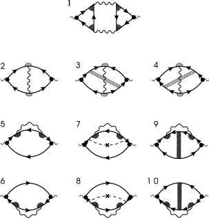
Figure 2: Feynman diagrams giving the leading-order corrections from the fluctuations to the sound attenuation. Diagram 1 is of the Aslamazov-Larkin (AL) type, diagrams 2-4 are of Maki-Thompson (MT) type, and the diagrams 5-10 are of the density of states (DOS) type. Solid lines are the normal state Green functions, wavy lines the fluctuation propagators, shaded semicircles and shaded rectangles the impurity ladder averagings, dashed lines with cross the single impurity scatterings, and bold circles the renormalized electron-phonon vertices. Adapted from Ref.LV01 .

Here, each wavy line in the figure corresponds to the fluctuation propagator (Cooper ladder) $L(q,\Omega_{k})$ which, as $T\rightarrow T_{c}$, has the form:

$$L(q,\Omega_{k})=-\left[\nu_{0}\left(\epsilon+\psi\left(\frac{1}{2}+\frac{|\Omega_{k}|}{4\pi T}\right)-\psi\left(\frac{1}{2}\right)\right.\right.$$ (11)

$$~{}~{}~{}~{}~{}~{}~{}-\left.\left.\frac{\langle({\Delta\xi}\left(\mathbf{q,p}\right)_{\left|p\right|=p_{F}})^{2}\rangle_{F.S.}}{(4\pi T)^{2}}\psi^{\prime\prime}\left(\frac{1}{2}+\frac{|\Omega_{k}|}{4\pi T}\right)\right)\right]^{-1},$$

where $\epsilon\approx(T-T_{c})/T_{c}$, and $\psi(z)$ is the digamma function. In the above Eq. (11), the angular average over the Fermi surface with the spectrum in Eq. (1) reads:

$$\langle({\Delta\xi}\left(\mathbf{q,p}\right)_{\left|p\right|=p_{F}})^{2}\rangle_{F.S.}$$ (12)

$$~{}~{}~{}~{}=\frac{1}{2}\left(\left(v_{F}q_{||}\right)^{2}+\left(4t_{\perp}\sin\left(q_{z}a/2\right)\right)^{2}\right)\equiv\tau^{-1}\widehat{D}q^{2},$$

where $\widehat{D}$ is a generalized diffusion operator.

Returning to Fig. 2, the shaded semicircles correspond to vertex corrections from impurity averaging and are given by:

$$\lambda(\mathbf{q},\varepsilon_{1},\varepsilon_{2})=\frac{|\tilde{\varepsilon}_{1}-\tilde{\varepsilon}_{2}|}{|\varepsilon_{1}-\varepsilon_{2}|+\frac{\widehat{D}q^{2}}{\tau^{2}|\tilde{\varepsilon}_{1}-\tilde{\varepsilon}_{2}|^{2}}\Theta(-\varepsilon_{1}\varepsilon_{2})}.$$ (13)

Diagrams 3, 4, 9 and 10 of Fig. 2 contain the impurity ladder in the particle-particle channel (shaded rectangle):

$$\Gamma_{c}(\mathbf{q};\varepsilon_{1},\varepsilon_{2}) = \frac{1}{2\pi\tau\nu_{0}}$$

$$\times \left(1-\frac{\Theta(-\varepsilon_{1}\varepsilon_{2})}{|\varepsilon_{1}-\varepsilon_{2}|\tau}\left(1-\frac{\widehat{D}q^{2}}{\tau(\varepsilon_{1}-\varepsilon_{2})^{2}}\right)\right),$$

while diagrams 7 and 8 have a single impurity line, which corresponds to the factor $1/(2\pi\tau\nu_{0})$. One can see that all other insertions of impurity lines either lead to diagrams that vanish, or give negligible corrections.

IV Calculational details for the diagrams

IV.1 MT and DOS diagrams

We illustrate the procedure to evaluate the diagrams in Fig. 2 by finding the expression for diagram 2 (Maki-Thompson type). In analytical form it is given by the integral:

$$\Pi^{(MT)}(\omega_{\nu},k)$$ (15)

$$~{}~{}~{}~{}~{}~{}~{}~{}=2g^{2}\ T\sum_{\Omega_{k}}\int\frac{d^{3}q}{(2\pi)^{3}}L(q,\Omega_{k})K(q,\Omega_{k},\omega_{\nu}),$$

where

$$K(q,\Omega_{k},\omega_{\nu})=T\sum_{\varepsilon_{n}}\lambda(q,\varepsilon_{n},\Omega_{k}-\varepsilon_{n})\lambda(q,\varepsilon_{n}+\omega_{\nu},\Omega_{k}-\varepsilon_{n}-\omega_{\nu})$$ (16)

$$~{}~{}~{}~{}~{}~{}\times\int\frac{d^{3}p}{(2\pi)^{3}}\cos\left(p_{z}a\right)\cos\left((q_{z}-p_{z})a\right)G(p,\varepsilon_{n})G(p+k,\varepsilon_{n}+\omega_{\nu})G(q-p,\Omega_{k}-\varepsilon_{n})G(q-p-k,\Omega_{k}-\varepsilon_{n}-\omega_{\nu}).$$

For simplicity, and as in experiment, usherb we assume that the sound propagates in the direction perpendicular to the conducting layers, so that $\mathbf{k}$ has only one component: $\mathbf{k}=(0,k_{z})$. The most singular contribution from the fluctuation propagator $L(\mathbf{q},\Omega_{k})$ comes from $\mathbf{q}\rightarrow 0$. Therefore, one can neglect the $\mathbf{q}$-dependence in the electron Green functions. We also set $\Omega_{k}=0$ LV01 since superconducting fluctuations are important in the renormalized classical regime where the characteristic frequency for the pair propagator is less than temperature.

Performing the integration over $\mathbf{p}$ in Eq. (16) first, one has for $K(q,\omega_{\nu})\equiv K(q,0,\omega_{\nu})$:

$$K(q,\omega_{\nu})=m\cos(q_{z}a)T$$ (17)

$${\!\!\!\!\!\!\!\!\!}\times\sum_{\varepsilon_{n}}\frac{1}{\left(2|\varepsilon_{n}+\omega_{\nu}|+\widehat{D}q^{2}\right)}\frac{1}{\left(2|\varepsilon_{n}|+\widehat{D}q^{2}\right)}\frac{1}{|\widetilde{\varepsilon_{n}+\omega_{\nu}}|+|\widetilde{\varepsilon}_{n}|}~{}.$$

that is then divided into two parts. Namely, the first part has the summation in the interval $\varepsilon_{n}\in(-\infty,-\omega_{\nu})\cup[0,\infty)$, while in the second one the summation is done in the interval $\varepsilon_{n}\in[-\omega_{\nu},0)$,

$$K(q,\omega_{\nu})$$ (18)

$${\!\!\!\!\!\!\!\!\!}=2T\sum_{n=0}^{\infty}\frac{1}{\left(2\varepsilon_{n}+\omega_{\nu}+\widehat{D}q^{2}\right)}\frac{1}{\left(2\varepsilon_{n}+\widehat{D}q^{2}\right)}\frac{1}{2\varepsilon_{n}+\omega_{\nu}+\tau^{-1}}~{}$$

$$+\frac{T}{\omega_{\nu}+\tau^{-1}}\sum_{n=-\nu}^{-1}\frac{1}{\left(2\varepsilon_{n}+2\omega_{\nu}+\widehat{D}q^{2}\right)}\frac{1}{\left(-2\varepsilon_{n}+\widehat{D}q^{2}\right)}.$$

Each of these two contributions leads to a different temperature dependence. The limits of summation in the second part of Eq. (18) can be obtained by taking into account the fact that frequencies $\varepsilon_{n}=\pi T(2n+1)$ are of the fermionic type while the sound frequency $\omega_{\nu}=2\pi T\nu$ is bosonic. The summation over $\varepsilon_{n}$ in the second part of Eq. (18) results in:

$$-\frac{m\cos(q_{z}a)}{4\pi(1+\omega_{\nu}\tau)}\frac{\psi\left(\frac{1}{2}+\frac{\hat{D}q^{2}}{4\pi T}\right)-\psi\left(\frac{1}{2}+\frac{\hat{D}q^{2}+2\omega_{\nu}}{4\pi T}\right)}{(\hat{D}q^{2}+\omega_{\nu})}.$$ (19)

The analytical continuation of this sum involves some subtleties that are discussed in the Appendix.

One can see that as $T\rightarrow T_{c}$, the main $q$-dependence in Eq. (15) comes from the fluctuation propagator $L(q)$ and from the poles of $K(q,\omega_{\nu})$. Therefore, it generally suffices to expand the regular part of $K(q,\omega_{\nu})$ in powers of $q$ and to keep the very first non-vanishing terms of the expansion.

The singular part of Eq. (19) comes from taking the $q^{0}$-term of the numerator together with the diffusion pole $1/(\hat{D}q^{2}+\omega_{\nu})$ and analytically continuing them to real phonon frequencies. One arrives at integrals of the type:

$$\int\frac{d^{3}q}{(2\pi)^{3}}\frac{\cos(q_{z}a)}{\left(\hat{D}q^{2}+1/\tau_{\phi}\right)\left(\epsilon+\eta q_{||}^{2}+r\sin^{2}(q_{z}a/2)\right)}.$$ (20)

where $r=16t_{\perp}^{2}\eta/v_{F}^{2}\ll 1$ is the anisotropy parameter r , and $\tau_{\phi}$ is the phase-breaking time, which provides the convergence of the integrals over the pair momentum $q$ at small wave vector $q$. Thompson The coefficient $\eta$ has the meaning of the square of the effective coherence length $\xi$ in the isotropic 2D case: LV01

$$\eta\equiv\xi^{2}\left(T\tau\right)=-\frac{\left(\tau v_{F}\right)^{2}}{2}$$ (21)

$$\times\left.\left[\psi\left(\frac{1}{2}+\frac{1}{4\pi x}\right)-\psi\left(\frac{1}{2}\right)-\frac{1}{4\pi x}\psi^{{}^{\prime}}\left(\frac{1}{2}\right)\right]\right|_{x=T\tau}.$$

At $T=T_{c}\,,$ the anisotropy parameter can be written as $r=4\xi_{\perp}^{2}(0)/a^{2}$ where $\xi_{\perp}(0)$ is the Cooper pair size in the perpendicular $\left(z\right)$ direction. We will also use the phase-breaking parameter $\gamma_{\phi}=2\eta/(v_{F}^{2}\tau\tau_{\phi})$ instead of $\tau_{\phi}$.

The integral in Eq. (20) results in the so-called anomalous MT contribution. Note however that while the leading term in the expansion of the numerator of Eq. (19) gave the above result, Eq. (20), the $q^{2}$-term of the expansion cancels the diffusion pole. This “regular anomalous” term, whose analog was overlooked in early work on conductivity fluctuation corrections, VarlamovThanks results in the same type of integral as that given by the first part of Eq. (18) with $q=0$:

$$\int\frac{d^{3}q}{(2\pi)^{3}}\frac{\cos(q_{z}a)}{\epsilon+\eta q_{||}^{2}+r\sin^{2}(q_{z}a/2)}.$$ (22)

Together, these two terms give so-called regular MT contribution, which generally has weaker temperature dependence than the anomalous MT part.

The evaluation of the diagrams 5-8 of Fig. 2 results in the integrals of the type

$$\int\frac{d^{3}q}{(2\pi)^{3}}\frac{1}{\epsilon+\eta q_{||}^{2}+r\sin^{2}(q_{z}a/2)},$$ (23)

which give the density of states part of the fluctuation corrections.

The remaining $\mathbf{q}$-integration in Eqs. (20), (22), and (23) is similar to that encountered for the conductivity calculations and is described in much details in the review LV01 and in Ref. Dorin93 . We should emphasize that as $T\rightarrow T_{c}$, the main temperature dependence of the fluctuation diagrams comes from these integrals. The remaining “bubble”, which consists of Green functions and impurity lines, has a weaker dependence on $T\tau$. It provides the coefficient in front of the function of $\epsilon$.

In the conductivity calculation, one can drop the diagrams containing the impurity ladder (3, 4, 9 and 10 of Fig. 2). This is because they contain the integration of one vector vertex with the Green function triangle. Angular integration over $\mathbf{p}$ leaves only terms containing powers of the small factor $(v_{F}k\tau)$. In the general case of sound attenuation and propagation these diagrams would contribute, but for sound propagating perpendicular to the layers the integration over the open Fermi surface of the vertex $g\cos(p_{z}a)$ also leads to a vanishing contribution for diagrams 3, 4, 9 and 10 of Fig. 2 to leading order in $k\ell$.

The small $\omega$ expansions of the DOS diagrams 5, 6, and of the regular contributions to the MT diagram 2 each lead to zeroth-order terms, the combination of which does not sum to zero. One notices the difference with the conductivity calculation, where such a cancellation of zeroth-order terms ensures that there is no anomalous diamagnetism above $T_{c}$. The DOS diagrams 7, 8, and the anomalous part of the MT diagram 2 do not have zeroth-order terms that would contribute to the leading renormalization of the sound velocity.

IV.2 Aslamazov-Larkin diagram

Finally, let us consider the Aslamazov-Larkin (AL) diagram 1, which gives the main fluctuation correction to most of the transport phenomena. In the case of sound propagation perpendicular to the layers, the analytical expression for the AL diagram reads:

$$\Pi^{(AL)}(\omega_{\nu},k)=-2g^{2}\ T\sum_{\Omega_{k}}\int\frac{d^{3}q}{(2\pi)^{3}}B^{2}(q,\Omega_{k},\omega_{\nu})$$

$$~{}~{}~{}~{}~{}~{}~{}~{}\times L(q,\Omega_{k})L(q,\Omega_{k}+\omega_{\nu}),$$ (24)

where

$$\!\!\!\!\!\!B(q,\Omega_{k},\omega_{\nu})=T\sum_{\varepsilon_{n}}\lambda(q,\varepsilon_{n}+\omega_{\nu},-\varepsilon_{n})\lambda(q,\varepsilon_{n},-\varepsilon_{n})$$ (25)

$$\!\!\!\!\!\!\times\int\frac{d^{3}p}{(2\pi)^{3}}\cos(p_{z}a)G(p,\varepsilon_{n})G(p,\varepsilon_{n}+\omega_{\nu})G(q-p,-\varepsilon_{n}),$$

In Eq. (25), we have neglected the $\Omega_{k}$-dependence of the electron Green functions. One can also set $\omega_{\nu}=0$ and expand $G(q-p,-\varepsilon_{n})$ in Eq. (25). Dorin93 For sound propagating perpendicular to the planes, we can use $r\mathbf{\ll}1$ (See Eq.(72)) to find the appropriate expansion parameter for $G(q-p,-\varepsilon_{n})$ appearing in the integral, namely:

$$\frac{\xi(\mathbf{q}-\mathbf{p})-\xi(\mathbf{p})}{\max\{\pi T,1/\tau\}}=\frac{2t_{\perp}\left(\cos((q_{z}-p_{z})a)-\cos(p_{z}a)\right)}{\max\{\pi T,1/\tau\}}.$$

After the angular integration in Eq. (25), the leading nonvanishing term reads:

$$B(q)=-\frac{4t_{\perp}\eta\nu_{0}(1-\cos(q_{z}a))}{v_{F}^{2}}.$$ (26)

Following the Ref. Dorin93 , one can integrate Eq.(IV.2), which after the analytic continuation and expansion in powers of $\omega$, results in the integral of the type:

$$\int\frac{d^{3}q}{(2\pi)^{3}}\frac{\sin^{4}(q_{z}a/2)}{\left(\epsilon+\eta q_{||}^{2}+r\sin^{2}(q_{z}a/2)\right)^{n+2}}$$ (27)

in the $n$-th order of $\omega$-expansion. To leading orders in $\omega$, the integrals in Eqs. (27) are not divergent at $\epsilon\rightarrow 0$. The resulting AL terms are finite and comparable with other fluctuation contributions.

V Results

In this section we collect the results for, in turn, the fluctuation corrections to the sound attenuation and then to the sound velocity.

V.1 Sound attenuation

The odd powers of the $\omega$-expansion of the analytically continued results for the diagrams of Fig. 2 give the fluctuation corrections to the imaginary part $\mathrm{Im}\left(\Pi^{R}(\omega)\right)$ of the retarded phonon self-energy. One can then use this result to obtain the sound attenuation from the imaginary part of the pole of the propagator, as in Eqs. (8) and (9).

All diagrams contribute to the polarization propagator to leading order in $\omega$. The different contributions to the sound attenuation coefficient are then extracted from the imaginary part of the retarded fluctuation polarization operator. In the most general form, they can be written as:

$$\alpha^{(\beta)}(T,\omega)=\frac{g^{2}\omega^{2}\nu_{0}}{\varepsilon_{F}v_{s}}\kappa_{att}^{(\beta)}(T\tau)f^{(\beta)}(\epsilon,r,\gamma_{\phi}),$$ (28)

where $\beta$ denotes the particular channel (DOS, rMT, aMT or AL). In Eq. (28), $f^{(\beta)}(\epsilon,r,\gamma_{\phi})$ means the function of temperature which comes from the integrals in Eqs. (20), (22), (23), and (27), and which also depends on the material properties. The coefficient $\kappa_{att}^{(\beta)}(T\tau)$ comes from the integration of Green functions and impurity blocks in the expression of the type (16). It has weaker temperature dependence at $\epsilon\rightarrow 0$ than $f^{(\beta)}(\epsilon,r,\gamma_{\phi})$, and it basically shows how the impurity concentration affects the result.

In the following, it will be more convenient to use the dimensionless parameter $\tilde{\eta}(T\tau)=\eta/\left(\tau v_{F}\right)^{2}$. We list here the functions $f^{(\beta)}$, which also appear in the conductivity calculation, Dorin93 and the coefficients $\kappa_{att}^{(\beta)}$. For the reader’s convenience, we also give the limiting expressions of $f^{(\beta)}$ which depend on the relation between $\epsilon$, $r$, and $\gamma_{\phi}$, where applicable.

DOS:

$$f^{(DOS)}(\epsilon,r)=\ln\left(\frac{2}{\sqrt{\epsilon}+\sqrt{\epsilon+r}}\right)$$ (29)

$$~{}~{}~{}~{}~{}~{}~{}~{}~{}~{}\approx-\frac{1}{2}\left\{\begin{array}[]{lll}&\ln r\ ,{}{}&\epsilon\ll r,\\ &&\\ &\ln\epsilon\ ,{}{}&r\ll\epsilon.\end{array}\right.$$ (33)

$$\kappa_{att}^{(DOS)}(x)=\frac{\psi^{{}^{\prime\prime}}\left(\frac{1}{2}\right)-2\pi x\psi^{{}^{\prime}}\left(\frac{1}{2}+\frac{1}{4\pi x}\right)}{8\pi^{2}x\tilde{\eta}(x)}$$

$$~{}~{}~{}~{}~{}~{}~{}~{}~{}~{}~{}~{}~{}~{}\approx\left\{\begin{array}[]{lll}&-{\ \mbox{\Large$\frac{28\zeta(3)}{\pi^{3}}$}},&~{}~{}x\ll 1,\\ &&\\ &-{\ \mbox{\Large$\frac{4\pi^{3}x^{2}}{7\zeta(3)}$}},&~{}~{}x\gg 1.\end{array}\right.$$ (37)

Regular part of MT:

$$f^{(rMT)}(\epsilon,r)=\frac{\left(\sqrt{\epsilon}-\sqrt{\epsilon+r}\right)^{2}}{r}$$ (38)

$$~{}~{}~{}~{}~{}~{}\approx\left\{\begin{array}[]{lll}&1\ ,{}{}&\epsilon\ll r,\\ &&\\ &{\mbox{\Large$\frac{r}{4\epsilon}$}}\ ,{}{}&r\ll\epsilon.\end{array}\right.$$ (42)

$$\kappa_{att}^{(rMT)}(x)=-\frac{\pi^{3}x-2\pi x\psi^{{}^{\prime}}\left(\frac{1}{2}+\frac{1}{4\pi x}\right)+\psi^{{}^{\prime\prime}}\left(\frac{1}{2}\right)}{16\pi^{2}x\tilde{\eta}(x)}$$

$$~{}~{}~{}~{}~{}~{}~{}~{}~{}~{}~{}~{}~{}~{}\approx\left\{\begin{array}[]{lll}&{\mbox{\Large$\frac{14\zeta(3)}{\pi^{3}}$}},&~{}~{}x\ll 1,\\ &&\\ &{2x},&~{}~{}x\gg 1.\end{array}\right.$$ (46)

Anomalous part of MT:

$$f^{(aMT)}(\epsilon,r,\gamma_{\phi})=\frac{1}{r}\left(-1+\frac{\epsilon+r+\gamma_{\phi}}{\sqrt{\gamma_{\phi}(\gamma_{\phi}+r)}+\sqrt{\epsilon(\epsilon+r)}}\right)$$

$$~{}~{}~{}~{}~{}~{}~{}~{}~{}~{}~{}~{}~{}~{}~{}~{}~{}\approx\left\{\begin{array}[]{lll}&{\mbox{\Large$\frac{1}{\sqrt{r\gamma_{\phi}}}$}}\ ,{}{}&\epsilon\ll\gamma_{\phi}\ll r,\\ &&\\ &{\mbox{\Large$\frac{1}{\sqrt{r\epsilon}}$}}\ ,{}{}&\gamma_{\phi}\ll\epsilon\ll r,\\ &&\\ &{\mbox{\Large$\frac{1}{2\epsilon}$}}\ ,{}{}&\gamma_{\phi}\ll r\ll\epsilon,\\ &&\\ &{\mbox{\Large$\frac{1}{2\gamma_{\phi}}$}}\ ,{}{}&\epsilon\ll r\ll\gamma_{\phi},\\ &&\\ &{\mbox{\Large$\frac{r}{8\gamma_{\phi}\epsilon}$}}\ ,{}{}&r\ll{\mbox{min}}\{\gamma_{\phi},\epsilon\}.\end{array}\right.$$ (56)

$$\kappa_{att}^{(aMT)}=-\frac{\pi}{4}.$$ (57)

AL:

$$f^{(AL,\alpha)}(\epsilon,r)=\frac{1}{r}\left(1-\sqrt{\frac{\epsilon}{\epsilon+r}}\left(1+\frac{r}{2(\epsilon+r)}\right)\right)$$

$$~{}~{}~{}~{}~{}~{}\approx\left\{\begin{array}[]{lll}&{\mbox{\Large$\frac{1}{r}$}}\ ,{}{}&\epsilon\ll r,\\ &&\\ &{\mbox{\Large$\frac{3r}{8\epsilon^{2}}$}}\ ,{}{}&r\ll\epsilon.\end{array}\right.$$ (61)

$$\kappa_{att}^{(AL)}=\frac{\pi}{8}.$$ (62)

The fluctuation terms scale like $\omega^{2}$ just as in the corresponding normal metal case without fluctuation correction.

V.2 Sound velocity

The renormalization of the phonon frequency $\omega(k)$ obtained from Eq. (10) provides the fluctuation corrections to the sound velocity when we use $\omega(k)=v_{s}k$. It should be emphasized that there is no anomalous MT term in leading (zeroth) order of $\omega$, while to higher order of $\omega$ all types of temperature dependences appear. To leading order $\omega^{0}$ the non-zero terms give, for $\Delta\omega/\omega=\left(\omega-\omega_{0}\right)/\omega_{0}$, the expressions in a form:

$$\frac{\Delta\omega^{(\beta)}(T,\omega)}{\omega}=\frac{\Delta v_{s}^{(\beta)}\left(T,\omega\right)}{v_{s}}$$ (63)

$$~{}~{}~{}~{}~{}~{}~{}~{}~{}~{}~{}~{}=\frac{g^{2}T\nu_{0}}{\varepsilon_{F}}\kappa_{v}^{(\beta)}f^{(\beta)}(\epsilon,r,\gamma_{\phi}),$$

For DOS, rMT and aMT terms, the temperature functions $f^{(\beta)}(\epsilon,r,\gamma_{\phi})$ are given by Eqs. (29), (38) and (V.1), respectively. The temperature function $f^{(AL,v)}(\epsilon,r)$ for the AL diagram is given by the Eq. (67), which is different from that for attenuation (V.1). We then obtain for the coefficients $\kappa_{v}^{(\beta)}$:

DOS:

$$\kappa_{v}^{(DOS)}=1,$$ (64)

Regular part of MT:

$$\kappa_{v}^{(rMT)}=-\frac{1}{2},$$ (65)

Anomalous part of MT:

$$\kappa_{v}^{(aMT)}=0,$$ (66)

AL:

$$\kappa_{v}^{(AL)}f^{(AL,v)}(\epsilon,r)$$ (67)

$$~{}~{}~{}~{}~{}~{}~{}=-\left(1+\frac{2\epsilon}{r}\left(-1+\sqrt{\frac{\epsilon}{\epsilon+r}}\right)\right)$$

$$~{}~{}~{}~{}~{}~{}~{}~{}~{}~{}~{}\approx-\left\{\begin{array}[]{lll}&1\ ,{}{}&\epsilon\ll r,\\ &&\\ &{\mbox{\Large$\frac{3r}{4\epsilon}$}}\ ,{}{}&r\ll\epsilon.\end{array}\right.$$ (71)

VI Discussion

Comparison of the normal state results without fluctuation corrections found in Sec. II with Eqs. (28) and (63) above show that the fluctuation corrections are smaller than the normal state contribution by a factor of $T/\varepsilon_{F}$. For layered organics, the Fermi surface parameters of Ref. Dressel lead to $T/\varepsilon_{F}\sim 10^{-2}$. The temperature functions $f^{(\beta)}$ increase this ratio at $T\rightarrow T_{c}$, thus making the fluctuation corrections experimentally measurable.

It can be seen from the results of previous section that it is the $\kappa^{(\beta)}(T\tau)$ coefficients that determine the sign of the fluctuation sound attenuation and sound velocity. The coefficients for sound attenuation $\kappa_{att}^{(\beta)}(T\tau)$ in Eq. (28) have weaker temperature dependence than that of the functions $f^{\beta}$. One can see that these coefficients in all fluctuation diagrams are finite as $(T\tau)\rightarrow 0$, and that they are of the same order of magnitude in this limit. In the opposite (clean) limit $(T\tau)\gg 1$, these coefficients increase as a power law of $(T\tau)$. We recall that there is an analogous formal divergence of the DOS and MT coefficients Dorin93 in the fluctuation conductivity but in that case they cancel each other in the limit $(T\tau)\gg 1$. In our case, the formal extension of our results to the limit $(T\tau)\gg 1/\sqrt{\epsilon}$ would be incorrect because the local approximation for the fluctuation propagator (11) and the impurity vertex (13) have a natural limit of validity $(T\tau)\ll 1/\sqrt{\epsilon}$ (the so-called local clean case). LSV00

In contrast to the coefficients for sound attenuation $\kappa_{att}^{(\beta)}(T\tau)$, the coefficients in the case of sound velocity, $\kappa_{v}^{(\beta)}$ in Eq. (63), do not depend on $T\tau$, thus simplifying the estimation of the sound velocity corrections in particular materials.

The overall magnitude of the fluctuation correction is given mainly by the temperature functions $f^{(\beta)}$. These functions depend on the anisotropy parameter $r$ and the phase-breaking time $\tau_{\phi}$, which are defined by the intrinsic material properties. The temperature function corresponding to a given type of diagram is identical for sound attenuation and velocity, except for the AL contribution which has temperature dependences that differ. In general, all the fluctuation terms remain finite as $T\rightarrow T_{c}$. The asymptotics of the corresponding temperature functions have been given in the preceding section and they were also discussed elsewhere. Dorin93

Figure 3: The temperature dependence of $f^{(DOS)}$ at various values of anisotropy parameter $r=10^{-1}\ldots 10^{-4}$.

Figure 4: The temperature dependence of $f^{(rMT)}$ at various values of anisotropy parameter $r=10^{-1}\ldots 10^{-4}$.

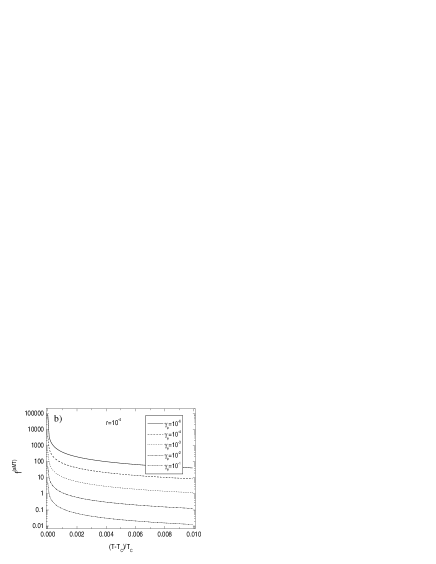
Figure 5: The temperature dependence of $f^{(aMT)}$ a) at fixed realistic $\gamma_{\phi}=0.1$ and at various values of anisotropy parameter $r=10^{-1}\ldots 10^{-4}$, b) at most realistic for the $\kappa$-(ET)₂ family compounds $r=10^{-4}$ and at various $\gamma_{\phi}=10^{-1}\ldots 10^{-6}$.

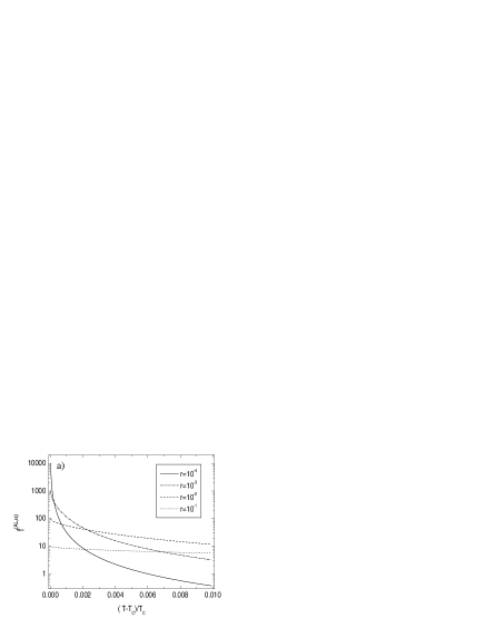
Figure 6: The temperature dependence of AL contributions a) to the sound attenuation $f^{(AL,\alpha)}$, b) to the sound velocity $f^{(AL,v)}$, at various values of anisotropy parameter $r=10^{-1}\ldots 10^{-4}$.

The functions $f^{\left(\beta\right)}$ also describe the crossover between two and three dimensions, where by three-dimensions we mean that the superconducting correlation length is much larger than the interlayer spacing. The two-dimensional behavior corresponds to $\varepsilon\gg r$ and the three-dimensional behavior to the opposite limit $r\gg\varepsilon$. The crossover occurs at $\varepsilon\sim r$, namely when the superconducting correlation length $\xi_{\perp}(0)\left|\varepsilon\right|^{-1/2}$ in the perpendicular direction becomes of the order of the interplane spacing.

In order to compare the contributions from different diagrams, we consider a range of parameters which is realistic for layered organic superconductors. The estimation for the anisotropy $t_{||}/t_{\perp}\approx 4000$, where $t_{||}$ is the intralayer transfer integral, is in agreement with the magnetoresistance data for $\kappa$-(ET)₂Cu(NCS)₂. Singleton This gives an anisotropy parameter of the order of $r{\ \gtrsim\ }10^{-4}$.

Concerning the scattering time, its estimate Singleton_tau from Shubnikov-de Haas experiments in $\kappa$-(ET)₂ materials gives $\tau\approx 3\;ps$, which leads to $T\tau\sim 1$ at $T\geq T_{c}$.

The phase-breaking time $\tau_{\phi}$ can be estimated from the experimental data on fluctuation contribution to transport coefficients using the appropriate expression for the MT diagram. The analysis of the magnetoresistance data on YBCO in Ref. Larkin_tau , which included AL and MT contributions, resulted in values $\tau_{\phi}\sim 1/T$. Later on, the authors of Ref. Dorin93 claimed that neglecting the orbital pair breaking effects while leaving the Zeeman contribution to the MT diagram in Ref. Larkin_tau can be incorrect. Hence, they extended the range of the realistic values of $\tau_{\phi}$ to $\tau_{\phi}{\ \lower-1.2pt\vbox{\hbox{\hbox to0.0pt{$<$\hss}\lower 5.0pt\vbox{\hbox{$\sim$}}}}\ }10/T$ with $\tau_{\phi}\sim 100/T$ being still acceptable for the analysis. Dorin93 A similar estimate was chosen by the authors of Ref. Sauls_tau to predict the magnitude of the fluctuation corrections to the nuclear spin-lattice relaxation rate and the NMR Knight shift in high-$T_{c}$ cuprates. To the best of our knowledge, no relevant analysis in layered organic materials have been reported to date. However, it is known that the phase-breaking time should satisfy the relation $\tau_{\phi}>\tau$. Without loss of generality then, we assume that pair breaking by inelastic scattering is weak enough and we consider $\gamma_{\phi}\ \sim 10^{-3}...10^{-2}$.

The aMT contribution vanishes to leading order, $\omega^{0}$, for sound velocity. With the above estimation for the anisotropy parameter, one can see that the AL part as well as the regular MT part give the least important non-vanishing contributions to sound velocity (order $\omega^{0}$). Indeed, $\lim_{\varepsilon\rightarrow 0}f^{(rMT)}(\varepsilon,r)={\ \lim_{\varepsilon\rightarrow 0}}f{{}^{(AL,v)}(\varepsilon,r)=1}$ at any $r$, while for the DOS contribution, $\lim_{\varepsilon\rightarrow 0}f^{(DOS)}(\varepsilon,r)=(1/2)\ln(4/r)\approx 5$ at $r\sim 10^{-4}$.

For sound attenuation the contribution of the AL term can be significant near $T_{c}$, by contrast to its contribution to the sound velocity, since $\lim_{\varepsilon\rightarrow 0}f^{(AL,\alpha)}(\varepsilon,r)=1/r$. However, it decays much faster than all other fluctuation terms above $T_{c}$: $f^{(AL,\alpha)}(\epsilon=0.002)/f^{(AL,\alpha)}(\epsilon=0.01)\simeq 23$ with $\lim_{r/\varepsilon\rightarrow 0}f^{(AL,\alpha)}(\varepsilon)\sim 1/\epsilon^{2}$. At the same time, at $\gamma_{\phi}\sim 10^{-3}...10^{-2}$ and $r\sim 10^{-4}$, we see that the anomalous MT temperature function is large, $f^{(aMT)}(\epsilon=0)\approx 500$ at $\gamma_{\phi}\sim 10^{-3}$ and $f^{(aMT)}(\epsilon=0)\approx 50$ at $\gamma_{\phi}\sim 10^{-2}$. Thus, at some $\gamma_{\phi}$, the aMT can be much larger than all other contributions. However, while it is quite large at $\epsilon=0$, the aMT part decreases with increasing $T$ faster than the DOS contribution. Indeed, at $r=10^{-4}$, the ratio $f^{(DOS)}(\epsilon=0.002)/f^{(DOS)}(\epsilon=0.01)\simeq 1.3$ shows that the DOS contribution has not changed much in that temperature range while the corresponding ratio for aMT is $f^{(aMT)}(\epsilon=0.002)/f^{(aMT)}(\epsilon=0.01)\simeq 5$ for the same $r$ and in the relevant range of $\gamma_{\phi}$. In other words, the logarithmic asymptotics (29) of the DOS diagram at $r/\epsilon\rightarrow 0$ wins over the power-law dependencies of the aMT term (V.1).

One can see that next order terms in the frequency expansion for the sound velocity and sound attenuation would contain the factor $(\omega/T)^{2n}$, where $n=1,2,\ldots$. The typical ultrasound frequency is of the order of $\omega\sim 100$ $\mathrm{MHz}$. At $T\gtrsim T_{c}\simeq 10\;\mathrm{K}$, the relevant frequency to temperature ratio is thus of the order $(\omega/T)^{2}\sim 10^{-7}$. One can check, for example, that in order to compensate for such a small factor, the parameter $\gamma_{\phi}$ in the anomalous MT term at $r\sim 10^{-4}$ should be as small as $10^{-10}$, corresponding to unreasonably large $\tau_{\phi}\sim 10^{8}\tau$. We conclude that, in our model, the sound velocity should be increased by the fluctuation corrections given by the DOS term.

Finally we would like to comment on the applicability of our model with regard to the character of interlayer electron transport in organic conductors, a subject which is still hotly debated. The interlayer tunneling of electrons can be coherent or incoherent (see Refs. Timusk_organics ; MosesMcKenzie and references therein). Following the terminology of Ref. MosesMcKenzie , we should distinguish between two limiting cases of incoherent interlayer transport, strongly and weakly incoherent. First, in the strongly incoherent case the intralayer electron momentum is not conserved in the tunneling processes between adjacent layers because the tunneling can be accompanied by strong elastic or inelastic processes. In this case the motion of electrons between the layers is diffusive and the electron band states in the $z$ direction and the corresponding Fermi surface cannot be defined. Our model is invalid in that limit. It is valid, however, in the second case, namely for weakly incoherent tunneling, that occurs when $\tau t_{\perp}\ll 1.$ In that case the intralayer electron momentum is conserved in the tunneling process and the electron wave function in adjacent layers has some overlap, but there are many in-plane collisions between tunneling events. Our approach is also valid obviously in the coherent case where $\tau t_{\perp}\gg 1$.

It is clear from our results that we can also consider two other limiting cases, namely the clean limit ($T\tau\gg 1$) and the dirty limit ($T\tau\ll 1$). The latter always corresponds to weakly incoherent tunneling while both coherent and weakly incoherent tunneling can occur in the former. This can be explained as follows. We have assumed throughout that $r\ll 1$. That parameter takes the following limiting forms: Dorin93

$$r=\frac{4\xi_{\perp}^{2}(0)}{a^{2}}\sim\left\{\begin{array}[]{cc}{\mbox{\Large$\frac{t_{\perp}^{2}\tau}{T}$ }},&T\tau\ll 1\\ &\\ {\mbox{\Large$\frac{t_{\perp}^{2}}{T^{2}}$ }},&T\tau\gg 1\end{array}\right.$$ (72)

where at $T=T_{c}$, $\xi_{\perp}(0)$ is the size of the Cooper pair perpendicular to the plane. The conditions $r\ll 1$ , and $T\tau\ll 1$, corresponding to dirty case, are consistent only with the weakly incoherent tunneling since they lead to $\left(\tau t_{\perp}\right)^{2}\ll T\tau\ll 1$. On the other hand, for $T\tau\gg 1$ the condition $r\ll 1$ is consistent with both coherent and weakly incoherent tunneling. This explains why in the preceeding discussion we distinguished only between the clean and dirty limits. Note that the crossover from clean to dirty limit occurs at $v_{F}/T\sim v_{F}\tau$, namely when the elastic mean free path becomes smaller than the thermal de Broglie wavelength.

In summary, the superconducting fluctuation corrections to the sound attenuation, in a realistic range of parameters, are given by the sum of the DOS, anomalous MT and AL terms, which decrease the normal state attenuation. In contrast, to leading order in $\omega$, the corrections to the sound velocity are given by DOS diagrams, because the expansion for the anomalous MT diagram begins at order $\omega$ while the AL diagram is small to this order.

VII Conclusion

We calculated, in the hydrodynamic limit $\omega\tau\ll 1$ and $k\ell\ll 1$, the effect of superconducting fluctuations on longitudinal sound propagating perpendicular to the layers of quasi two-dimensional systems above $T_{c}$. This corresponds to the experimentally realizable situation. The detailed results for the sound attenuation coefficient $\alpha$ and the sound velocity renormalization $\Delta v_{s}/v_{s}$ are summarized in section V.  In short, there are four types of temperature dependences coming respectively from a) the density of states diagrams, b) the regular contribution of the Maki-Thompson diagram, c) the anomalous contribution of the Maki-Thompson diagram and d) from AL diagram. These contributions have different signs and their magnitudes strongly depend on material properties such as anisotropy and phase-breaking processes. For longitudinal sound propagating perpendicular to the layers, the open Fermi surface condition leads to a suppression of the divergent contributions to leading order, so that fluctuation corrections to sound attenuation are expected to generally be much smaller than the fluctuation corrections to conductivity.

The leading temperature dependences with respect to $T_{c}$ of the fluctuation corrections to the sound attenuation have the same $\omega^{2}$ scaling with frequency as in the impure (dirty) metal without fluctuation correction. To this order in $\omega$, all four types of temperature contributions are present. As we move close to $T_{c}$, the fluctuation contribution decreases the sound attenuation below its normal state level, at least for realistic values of the material parameters.

The leading fluctuation correction to the sound velocity does not depend on $\omega$, just like the normal state term. To this order, there are only three types of temperature dependences coming from the density of states diagram, AL diagram and from the regular contribution of the Maki-Thompson diagram. The overall fluctuation correction in realistic material situation should be dominated by the density of states contribution and should increase the sound velocity as we approach $T_{c}$. The anomalous contribution of the Maki-Thompson diagram is proportional to $\left(\omega/T\right)^{2}$ and generally can be neglected unless phase breaking is extremely low. Further details of our calculations may be found in Ref. web .

It should be noted that our results on sound attenuation are in qualitative agreement with the preliminary experimental data. KFrikash These experiments are currently in progress. The detailed analysis including the comparison with the present theory will be published elsewhere.

To make actual comparisons with experiment, one may need to consider several other physical effects. For example, strongly incoherent interplane tunneling MosesMcKenzie and $d$-wave superconductivity Mayaffre95 may have to be considered. In addition, one may need to include in the fluctuation propagator Eq. (11) mode-coupling terms that will allow to go beyond mean-field theory in the description of the crossover from two to three dimensions.

Appendix A On the analytical continuation of the digamma function of complex argument

We shall discuss an important mathematical issue occurring in the evaluation of the anomalous MT contribution (18) and its further analytic continuation. Namely, let us look at the typical sum over the fermionic Matsubara frequencies:

$$T\sum_{n=0}^{\nu-1}\frac{1}{\varepsilon_{n}}.$$ (73)

The expression (73) appears if one decomposes into partial fractions the initial sum over $\varepsilon_{n}$ in the anomalous part of the Maki-Thompson diagram and neglects the small terms $\sim\hat{D}q^{2}$ in them. One can easily evaluate the sum (73) using the well-known representation of the digamma function:

$$T\sum_{n=0}^{\nu-1}\frac{1}{\varepsilon_{n}}=\frac{1}{2\pi}\left\{\psi\left(\frac{1}{2}+\nu\right)+2\ln 2+\gamma\right\},$$ (74)

where $\gamma=0.577216$ is the Euler constant. Here $\nu$ comes from the external bosonic Matsubara frequency $\omega_{\nu}=2\pi T\nu$, with $\nu$ an integer. At the same time, it is easy to see that the straightforward change of variable $n=-n^{\prime}-1$ transforms the initial expression (73) in a way that one obtains the alternate result:

$$T\sum_{n=0}^{\nu-1}\frac{1}{\varepsilon_{n}}\equiv-T\sum_{n^{\prime}=-\nu}^{-1}\frac{1}{\varepsilon_{n}^{\prime}}$$ (75)

$$~{}~{}~{}~{}~{}~{}~{}~{}~{}~{}~{}=\frac{1}{2\pi}\left\{\psi\left(\frac{1}{2}-\nu\right)+2\ln 2+\gamma\right\}.$$

As long as we deal with the Matsubara frequencies $\omega_{\nu}=2\pi T\nu$ these two results Eq. (74) and Eq. (75) are equivalent because of the relation

$$\psi\left(\frac{1}{2}-z\right)=\psi\left(\frac{1}{2}+z\right)+\pi\tan(\pi z),$$ (76)

and the fact that $\tan(\pi z)=0$ when $z=\nu$ is an integer. Therefore, at this stage we are free to choose either Eq. (74) or Eq. (75) as the result of the summation. The distinction appears when one tries to do the analytic continuation to real frequencies $i\omega_{\nu}\rightarrow\omega+i\eta$. After analytic continuation, Eqs. (74) and (75), which we obtained from the same diagram, are not equal to each other anymore. Indeed, for non-integer $\nu$, $\psi\left(\frac{1}{2}-z\right)=\psi\left(\frac{1}{2}+z\right)$ is not true anymore, as one can see from Eq. (76).

It is crucial to choose either Eq. (74) or Eq. (75) as the result of the summation before we do the analytic continuation. The choice is determined by whether we want the advanced or the retarded response function. Indeed, consider Eqs. (74) and (75) as general response functions $\chi^{M}(\omega_{\nu})=\chi(z)|_{z=i\omega_{\nu}}\varpropto\psi\left(\frac{1}{2}\pm\nu\right)$ on the Matsubara frequency domain $\omega_{\nu}$. If we then analytically continue the argument $z=i\omega_{\nu}\rightarrow\omega+i\eta$ of $\psi\left(1/2-iz/(2\pi T)\right)$, the poles of resulting function are all located below the real axis of the complex plane thus giving us the retarded function $\chi^{R}(\omega)$. On the other hand, the analytic continuation $z=i\omega_{\nu}\rightarrow\omega-i\eta$ of the argument of $\psi\left(1/2+iz/(2\pi T)\right)$ gives us the advanced response because all its poles are located in the upper half-plane.

We thus conclude that if the digamma function appears in our calculations, we are free to use either Eqs. (74) or (75) because they are equivalent, as long as we deal with Matsubara frequencies. However, before doing the analytic continuation, we have to decide whether we need the advanced or the retarded function. If we want the retarded function, we use the rule given by Eq. (74) and deal only with digamma functions of the type $\psi(1/2+\nu)$. Otherwise, use $\psi(1/2-\nu)$ to obtain the advanced response.

References

- (1) L.G. Aslamazov and A.I. Larkin, Soviet Solid State 10, 875 (1968); Phys. Lett. 26A, 238 (1968).
- (2) K. Maki, Progr. Theor. Phys. (Kyoto) 39, 897 (1968); 40, 193 (1968).
- (3) R.S. Thompson, Phys. Rev. B 1, 327 (1970).
- (4) A.I. Larkin and A.A. Varlamov, Fluctuation Phenomena in Superconductors, in Handbook on Superconductivity: Conventional and Unconventional Superconductors ed. by K.-H. Bennemann and J.B. Ketterson (Springer, 2002).
- (5) J.E. Graebner, R.C. Haddon, S.V. Chichester, and S.H. Glarum, Phys. Rev. B 41, 4808 (1990); D.E. Farrell, C.J. Allen, R.C. Haddon, and S.V. Chichester, Phys. Rev. B 42, 8694 (1990); M. Lang, F. Steglich, N. Toyota, and T. Sasaki, Phys. Rev. B 49, 15227 (1994); S. Friemel, C. Pasquier, Y. Loirat, and D. Jérome, Physica C: Superconductivity 259, 181 (1996); S. Belin, K. Behnia, and A. Deluzet, Phys. Rev. Lett. 81, 4728 (1998); N.J. Clayton, H. Ito, S.M. Hayden, P.J. Meeson, M. Springford, and G. Saito, Phys. Rev. B 65, 064515 (2002).
- (6) K. Frikach, M. Poirier, M. Castonguay, and K.D. Truong Phys. Rev. B 61, R6491 (2000), D. Fournier, M. Poirier, M. Castonguay, and K. Truong, Phys. Rev. Lett. 90, 127002 (2003).
- (7) K. Frikach, PhD thesis, Université de Sherbrooke 2001 (unpublished).
- (8) M.B. Walker, M.F. Smith, and K.V. Samokhin, Phys. Rev. B 65, 014517 (2002).
- (9) S. Yip, Phys. Rev. B 41, 2612 (1990). P. Carretta, A. Rigamonti, A.A. Varlamov, and D.V. Livanov, Phys. Rev. B 54, R9682 (1996).
- (10) M. Eschrig, D. Rainer, and J.A. Sauls, Phys. Rev. B 59, 12095 (1999).
- (11) A.B. Pippard, Philosophical magazine 46, 1104 (1955).
- (12) T. Tsuneto, Phys. Rev 121, 402 (1961).
- (13) A. Schmid, Z. Physik 259, 421 (1973).
- (14) B.G. Kotliar and T.V. Ramakrishnan, Phys. Rev. B 31, 8188 (1985).
- (15) M.Yu. Reizer, Phys. Rev. B 40, 7461 (1989).
- (16) L.G. Aslamazov and A.A. Varlamov, Sov. Phys. JETP 77, 2410 (1979).
- (17) E.I. Blount, Phys. Rev. 114, 418 (1959).
- (18) S. Barišić, Phys. Rev. B 5, 932 (1972), ibid. 941.
- (19) W.P. Su, J.R. Schrieffer, and A.J. Heeger, Phys. Rev. Lett. 42, 1698 (1979).
- (20) A.A. Abrikosov, L.P. Gorkov, and I.E. Dzyaloshinski, ”Methods of the quantum field theory in statistical physics”, Dover Publications, New York (1963).
- (21) A.A. Abrikosov, Introduction to the Theory of Normal Metals (Academic Press, New York, 1972).
- (22) V.V. Dorin, R.A. Klemm, A.A. Varlamov, A.I. Buzdin, and D.V. Livanov, Phys. Rev. B 48, 12951 (1993).
- (23) R.A. Klemm, M.R. Beasley, and A. Luther, Phys. Rev. B 8, 5072 (1973); R.A. Klemm, J. Low Temp. Phys. 16, 381 (1974).
- (24) We thank A.A. Varlamov for pointing this out.
- (25) M. Dressel, O. Klein, G. Grüner, K.D. Carlson, H.H. Wang, and J.M. Williams, Phys. Rev. B 50, 13603 (1994).
- (26) D.V. Livanov, G. Savona, and A.A. Varlamov, Phys. Rev. B 62, 8675 (2000).
- (27) J.M. Caulfield, W. Lubczynski, F.L. Pratt, J. Singleton, D.Y.K. Ko, W. Hayes, M. Kurmoo, and P. Day, J. Phys.: Condens. Matter 6, 2911 (1994); John Singleton, P.A. Goddard, A. Ardavan, N. Harrison, S.J. Blundell, J.A. Schlueter, and A.M. Kini, Phys. Rev. Lett. 88, 037001 (2002).
- (28) J. Singleton, C.H. Mielke, W. Hayes, and J.A. Schlueter, J. Phys.: Cond. Matter 15, L203 (2003).
- (29) J.B. Bieri and K. Maki, Phys. Rev. B 42, 4854 (1990); J.B. Bieri, K. Maki, and R.S. Thompson, Phys. Rev. B 44, 4709 (1991); A.G. Aronov, S. Hikami, and A.I. Larkin, Phys. Rev. Lett. 62, 965 (1989); ibid. 2336 (1989).
- (30) J.J. McGuire, T. Rõõm, A. Pronin, T. Timusk, J.A. Schueter, M.E. Kelly, and A.M. Kini, Phys. Rev. B 64, 094503 (2001).
- (31) P. Moses and R.H. McKenzie, Phys. Rev. B 60, 7998 (1999).
- (32) The Mathematica source files as well as .pdf version for the fluctuation corrections can be found at http://www.physique.usherb.ca/tremblay/pub/sound.html
- (33) D. Achkir, M. Poirier, C. Bourbonnais, G. Quiron, C. Lenoir, P. Batail, and D. Jérome, Phys. Rev. B 47, 11595 (1993); H. Mayaffre, P. Wzietek, D. Jérome, C. Lenoir, and P. Batail, Phys. Rev. Lett. 75, 4122 (1995); A. Carrington, I.J. Bonalde, R. Prozorov, R.W. Giannetta, A.M. Kini, J. Schlueter, H.H. Wang, U. Geiser, and J.M. Williams, Phys. Rev. Lett. 83, 4172 (1999).