Caloric Curves in two and three-dimensional Lennard-Jones-like systems including Long-range forces

Abstract

We present a systematic study of the thermodynamics of two and three-dimensional generalized Lennard-Jones ($LJ$) systems focusing on the relationship between the range of the potential, the system density and its dimension. We found that the existence of negative specific heats depends on these three factors and not only on the potential range and the density of the system as stated in recent contributions.

1 Introduction

In the last few years a lot of attention has been paid to Hamiltonian systems in which the interaction potential range is of the order of the size of the system. Typical examples include nuclei, metallic clusters and galaxies. In the first two cases the system under consideration is small comprising just a few (or less) hundreds of particles, while in the third one the range of the potential is long tsa1 ; curilef ; tsapre ; tamarit .

One of the main consequences of dealing with long-range Hamiltonian systems is the appearance of negative specific heats. Negative specific heats appear in the literature of small systems both in experimental D'agostino ; Haberland and theoretical Labastie ; gross studies. In particular, in a series of recent papers, we have found such a behavior for highly excited small Lennard Jones aggregates ($147$ particles) both free to expand and constrained in an spherical volume noneqfrag ; mison . In this case the standard ($12-6$) $LJ$ systems in $3$ dimensions qualifies as a short-ranged potential, since the exponent of the attractive term of the potential ($\alpha=6$) is greater than the dimension of the system ($d=3$). On the other hand, in tsa1 it is claimed, based on the numerical analysis of two-dimensional systems, that a negative specific heat region is present only if long-range forces are present. It is therefore necessary to make a complete study in order to clarify the interplay between the potential range and the thermodynamics of the system.

The presence of such a long range interaction in the system calls for a proper thermodynamical description. One can, for instance, try to use Tsallis statistics tsallis . However, ”small” systems can be also studied via micro-canonical statistics gross . Our studies and conclusions will be referred to the $N,V,E$ ensemble.

This work is organized as follows. In Section 2 we present the model, the interaction potential and the observables that we use in the calculations. In Section 3 we show the results of our simulations for two and three-dimensional systems. Finally in Section 4 we present our conclusions.

2 The model

The system under study is composed by a gas of $147$ particles confined in a spherical box, defined by the Hamiltonian $H=K+V/\tilde{N}+V_{walls}$, where K is the kinetic energy and the interaction potential is given by $V=\Sigma v(r_{ij})$ with $v(r_{ij})=C_{\alpha}[\frac{\sigma}{r_{ij}}^{-12}-\frac{\sigma}{r_{ij}}^{-\alpha}](0\leq\alpha<12)$ and $C_{\alpha}=\epsilon(12^{12}/\alpha^{\alpha})^{1/(12-\alpha)}/(12-\alpha).$ The Lennard-Jones like potentials as a function of $r$ are shown in Fig. 1 for $d=3$, $N=147$, and several values of $\alpha$. We used a spherical confining wall via an external potential $V_{wall}\sim(r-r_{wall})^{-12}$ with a cut off distance $r_{cut}=1\sigma$. Energies are measured in units of the potential well ($\epsilon$), and the distance at which the potential changes sign ($\sigma$), respectively. The unit of time used is $t_{0}=\sqrt{\sigma^{2}m/48\epsilon}$.

The nonextensive scaling parameter, introduced in tsa1 , $\tilde{N}\equiv 1+d\int_{1}^{N^{1/d}}drr^{d-1-\alpha}$ is convenient to make the Hamiltonian formally extensive $\forall\alpha/d$ ($d$ is the dimensionality of the system).

The model is exactly the one introduced in tsa1 , and the particular case $\alpha=6$ recovers the celebrated Lennard-Jones model.

The set of classical equations of motion were integrated using the velocity Verlet algorithm, which preserves volume in phase space allen ; with an integration time step between $0.001t_{0}$ and $0.01t_{0}$ which guaranteed a conservation of the energy not worse than $0.01\%$. Initial conditions were constructed from the ground states of $LJ$ systems in $r-space$ and rescaling velocities with a Maxwellian distribution of velocities to the desired value of energy. All calculations were performed once the transient behavior was over.

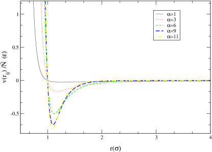
Figure 1: Set of generalized $LJ$ $3D$ potentials.

2.1 Discussion about the $\tilde{N}$ term

To properly understand the inclusion of the $\tilde{N}$ normalization term let’s remember the cluster expansion in real gases. By integrating in moments we end up with the proportionality of the partition function and the configuration integral

$$\frac{1}{\lambda^{3N}N!}\int{d^{3N}qexp[-\beta\Sigma v_{ij}]}$$ (1)

In the Van der Waals approximation

$$V(r) = \infty\quad\quad\quad r<r_{0}$$ (2)

$$exp[-\beta V(r)] \sim 1-\beta V(r)\quad r>r_{0}$$ (3)

It can be easily shown that

$$E-E_{ideal}=N_{pairs}<V(r)>$$ (4)

with $<V(r)>=\frac{4\pi}{V}\int{drr^{2}V(r)}$. We see that $\tilde{N}$ is a generalization of this term taking into account the adimensionalization and the finite number of particles. As the configurational integral is ill-defined for long-range potentials (decaying slower than $d$) thermodynamic quantities $A_{N}$ like the internal energy, the free energy, Gibbs energy, etc. associated with systems including long-range potentials scale like curilef

$$\frac{A_{N}}{N}\propto\int_{1}^{N^{1/d}}drr^{d-1-\alpha}=\frac{1}{d}\\ \frac{N^{1-\alpha/d}-1}{1-\alpha/d}$$ (5)

By normalizing the potential energy with $\tilde{N}$ the Hamiltonian is turned formally extensive.

2.2 The observables

The main observable to be extracted from our simulations is the caloric curve ($CC$), which is defined as the functional relationship between the temperature of the system and its energy in terms of the density i.e. $T(E,\rho)$, from which we define the specific heat as

$$C_{v}=\frac{1}{\partial T/\partial E)_{v}}$$ (6)

It is then clear that a $C_{v}<0$ will be obtained if and only if the $CC$ displays a loop.

It has recently been proposed that first order phase transitions would be univocally signed by the amount of fluctuations in the different subsystems in which the system can be subdivided gulmi_fluc . In particular, the relative kinetic energy fluctuation $A_{K}$ is defined as:

$$A_{K}=\frac{N\sigma^{2}_{K}}{T^{2}}$$ (7)

where $N$ is the number of particles, $\sigma_{K}$ the standard deviation of the kinetic energy per particle and $T$ the temperature of the system. Since kinetic energy fluctuations and the specific heat are related by lebowitz

$$N<\sigma_{K}^{2}>_{E}={\frac{d}{{2\beta^{2}}}}(1-{\frac{d}{{2C}}})$$ (8)

Negative values of the specific heat should be expected whenever $A_{K}$ exceeds the canonical value ($A_{K}=1.5\epsilon$ for $d=3$ and $A_{K}=1.0\epsilon$ for $d=2$) gulmi_fluc ; noneqfrag .

3 Results

3.1 Caloric Curves and Kinetic Energy Fluctuations in three dimensions

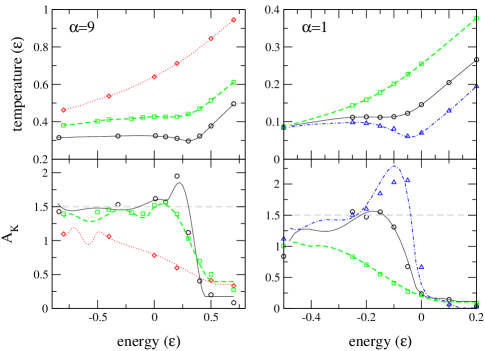
Figure 2: Caloric curves and relative kinetic energy fluctuations for $\alpha=9$, $\rho=0.01\sigma^{-3}$ (circles), $\rho=0.06\sigma^{-3}$ (squares) and $\rho=0.3\sigma^{-3}$ (diamonds) (left panels) and $\alpha=1$, $\rho=0.001\sigma^{-3}$ (triangles), $\rho=0.01\sigma^{-3}$ (circles), $\rho=0.06\sigma^{-3}$ (squares) (right panels).

We will first focalize in the study of three-dimensional systems. In Fig.2 we show the caloric curve for a system composed of $147$ particles with $\alpha=9$ (upper left panel) and for $\alpha=1$, a long-range potential (upper right panel). For future reference, it is interesting to notice that the case $\alpha=9$ for 3 dimensions would correspond to $\alpha=6$ in 2 dimension because for both the quotient $\frac{\alpha}{d}=3.$ It can be seen that a loop in the caloric curve is present in both cases only when the system density is low (notice the density differences in both panels). For a short-ranged potential the relationship between the caloric curves and the constraining volume has already been clarified (see noneqfrag ): The presence of a loop in the caloric curve can be related to the formation of drops in configuration space. When dealing with long-ranged potentials the scenario slightly changes, even though the clusters can not be completely isolated, we still have weakly-interacting clusters, they just need more room to accommodate. We will come back to this point later.

Figure 3: Range dependence of the caloric curves for $\rho=0.01\sigma^{-3}$, $d=3$.

In the lower panels of Fig. 2 we show $A_{K}$ for several densities (see caption for details). Whereas the symbols refer to calculations of $A_{K}$ via fluctuations (Eq.7) the lines show the corresponding $A_{K}$ estimations using the information provided by the caloric curves, through Eq.8. It is immediate that fluctuations are enhanced well above the canonical value for the cases where the caloric curve displays a loop.

In Fig.3 we show the dependence of the caloric curve with the range of the interaction for a constant density ($\rho=0.01\sigma^{-3})$, which correspond to a low density for all but the extremely long-range potential $(\alpha=1)$, reflected by the absence of a loop in the caloric corresponding curve. Also notice that the energy which points the entrance of the system into the vapor branch is an increasing function of the total energy for long-range systems ($\alpha\leq 3$) and then collapses to a constant value for the short-range cases studied.

3.2 Statistical inefficiency corrections

The importance of the loop in the caloric curve resides in the fact that it is a signal which identifies the presence of a first order phase transition for the corresponding density and lower ones. In Ref cheba the phase diagram for a pure $LJ$ system was constructed by analyzing different observables. As a consequence of this, the phase diagram was divided into three density regions. In the low density regime the $CC$ displays a loop whereas for higher densities the identification of the transition line was performed by a phase-space analysis. It is therefore relevant to study the relationship between the range of the potential and the density for which the loop disappears which we have called ’disjoint density $\rho_{dis}$’ since it acts like a separatrix between two regions of the phase diagram.

Up to this point we have identified the presence of negative specific heats via two independent signals: The presence of the loop in the $CC$ and abnormally large kinetic energy fluctuations $A_{K}$. We define $\rho_{dis}$ as the density at which the signals (presence of the loop including errors and relative fluctuations greater than the canonical value) either both disappear at the same time or they become inconsistent, i.e. a loop without big relative fluctuations or viceversa. It is worth to notice that only in a region in $\rho$-space very close to $\rho_{dis}$ these two signals can become inconsistent.

Special care should be taken because not only we are dealing with observables linked to mean values but to fluctuations (second moments), as well. In order to disregard erroneous results we performed a statistical inefficiency study, a tool which was introduced by Jacucci and Rahman rahman to estimate errors from correlated data series.

The block average procedure is used to calculate the error of a quantity $K$ computed from a correlated data series. In order to establish the error, the data are grouped into $b$ blocks of length $n_{b}$. We expect the averages of the data in each block no to be correlated for sufficiently long $n_{b}$. The block size ($n_{b}$) is used to obtain uncorrelated data (the statistical inefficiency $s$) for a quantity $K$ using:

$$s=\lim_{n_{b}\rightarrow\infty}\frac{n_{b}\sigma^{2}(<K>_{b})}{\sigma^{2}(K)}$$ (9)

where $\sigma^{2}(K)$ and $\sigma^{2}(<K>_{b})$ are given by:

$$\sigma^{2}(K)=\frac{1}{M}\sum_{i=1}^{M}(K_{i}-<K>_{total})^{2}$$ (10)

$$\sigma^{2}(<K>_{b})=\frac{1}{b}\sum_{j=1}^{b}(<K>_{j}-<K>_{total})^{2}$$ (11)

$<K>_{j}$ is the average of every block and $<K>_{total}$ is the average over the full data set of length $b*n_{b}=M$.

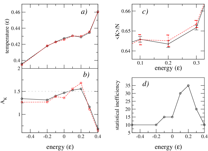
Figure 4: In this figure we show the results of the statistical inefficiency analysis for $\alpha=9,\rho=0.06\sigma^{-3}$. Panel a) shows the caloric curve for the raw data (full line, circles) and data taken via a random sampling (dashed line, squares). Panel b) shows the relative kinetic energy fluctuations for the same situations. In Panel c) we show more closely the differences between the random sampling and the coarse graining sampling (notice the errors in the random sampling case are bigger). Panel d) shows the statistical inefficiency as a function of the energy.

Having determined the value of statistical inefficiency, the simulation runs are divided into blocks of size $n_{b}$, and sampled either via a random sampling, where a single value is taken at random from each block, the data set taken as the set of such values; or coarse-graining, where the data set is taken as the set of block averages.

In Fig.4 we show the results of the statistical inefficiency analysis for $\alpha=9,\rho=0.06\sigma^{-3}$. We can see that the caloric curve does not change appreciably, we can not state the existence of the loop due to the numerical uncertainties involved (see panel $c$). Even though $A_{K}$ is more sensitive to numerical correlations between the data (it depends on both the first and second moments) this signal does not change qualitatively between the raw data and the random sampling. It is interesting to notice the behavior of the statistical inefficiency as a function of the system energy: There is a clear peak in the same region where the caloric curve displays a loop, showing that the transition from liquid-like to a gas-like system is in correspondence with an increase in the correlation time.

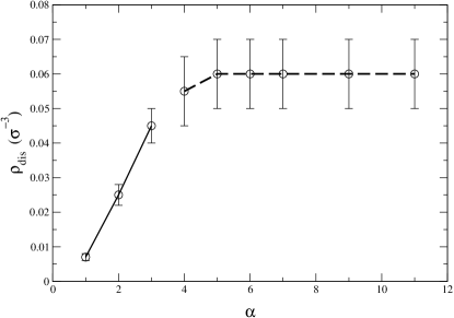
Figure 5: Disjoint density as a function of the potential range for $d=3$.

Using results obtained with the above-mentioned methodology, we show in Fig.5 $\rho_{dis}$ as a function of $\alpha$. We can see that there is a clear distinction between long-range and short-range systems: For long-range systems ($\alpha\leq 3$) $\rho_{dis}$ is an increasing function of $\alpha$ (a decreasing function of the potential range) which suggest that the loop acts as a pointer of ”surfaces”, since a long-range interaction system needs more volume to develop a structure with weakly interacting clusters. For short-range systems there is a collapse to a $\rho_{dis}=0.06\sigma^{-3}$ value.

Summarizing the results of this section , we have found from our calculations that in the case of constrained small three-dimensional systems negative specific heats appear for all ranges of the interaction potential, i.e. for all values of the parameter $\alpha$ for densities below an appropriate threshold for each case.

3.3 Two-dimensional systems

We now turn our attention to systems in two dimensions. In the upper panel of Fig.6 we show the range dependence of the caloric curves for a constant value of the density $\rho=0.01\sigma^{-2}$ for $N=100$ particles.

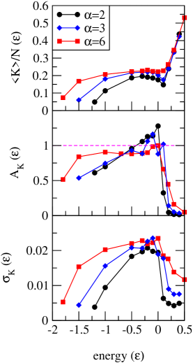
Figure 6: Temperature, Relative fluctuations of the kinetic energy and fluctuations of the kinetic energy as a function of the energy for $d=2,\rho=0.01\sigma^{-2}$.

It is immediate that there are differences between the three-dimensional and the two-dimensional case. In the former we found that if the density is low enough, then a loop in the Caloric Curve is present for every $\alpha$ ($\rho_{dis}$ being an increasing function of $\alpha$). On the other hand, for the two-dimensional case we found a loop for a long-range potential ($\alpha=2$), and also for a short-range case ($\alpha=3$, that correspond to a short-range potential in $d=2$). However the increase of $\alpha$ towards bigger values makes the depth of the loop almost vanish, which forbids us to identify negative values of $C_{v}$ due to the numerical uncertainties involved. Moreover, If we only take into account the range of the potential $\frac{\alpha}{d}$ (as was defined in tsa1 ) and we compare what happens for $two$-dimensional and $three$-dimensional systems, we realize that we have two different behaviors for the same value of the potential range. Recall from Fig.3 that the curve corresponding to $\alpha=9$, $d=3$ exhibit a clear loop; on the other hand from Fig.6 the case $\alpha=6$, $d=2$ presents no loop. This show that the existence of the loop is not only related to the range of the potential, but to the dimension of the system as well.

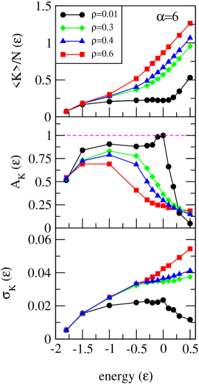
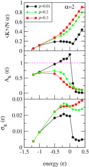
Figure 7: Temperature, Relative fluctuations of the kinetic energy, potential energy and standard deviation of the kinetic energy per particle as a function of the energy for $d=2$.

In brief, at variance with the three-dimensional case, in two dimensions the system does not display negative specific heats for all ranges of the interaction potential but only for $\alpha\leq 3$, partially confirming the results of tsa1 .

We now turn our attention to the analysis of the behavior of the quantity $A_{k}$ for the two-dimensional case. In the middle and lower panels of Fig.6 we show the relative fluctuations of the kinetic energy $A_{K}$ and the standard deviation of the kinetic energy per particle as a function of the energy for $d=2,\rho=0.01\sigma^{-2}$. We see once again that $A_{K}$ is a good signature of the presence of the loop. On the other hand, $\sigma$ is essentially the same for all curves shown (having and not having a loop). In the $3D$ $LJ$ case, it has been found cheba that this signal changes from displaying a loop to a monotonous increasing function of the energy at the critical density $\rho_{c}$. This picture is compatible with the left panel of Fig.7, where we show the density dependence of the caloric curves, $A_{K}$, and the standard deviation of the kinetic energy per particle for a short-range ($\alpha=6$, left panel) and a long-range ($\alpha=2$, right panel) case. It is worth to mention that it is only for the $\alpha=6$ system that we can make a correspondence with the phase diagram of a $LJ$ fluid. Nevertheless the right panel of Fig.7 show us that the scenario does not change qualitatively for long-range potentials between $d=2$ and $d=3$.

4 Conclusions

In this work we have undertaken a detailed numerical analysis of the thermodynamic behavior of finite confined systems in two an three dimensions at fixed $NVE$. Our goal was to study the behavior of the specific heat in terms of the density and dimension of the system. We identified negative specific heats by searching for loops in the corresponding caloric curves, and studying the relative kinetic energy fluctuations of the system, finding consistent results in both approaches. Special emphasis was taken in the statistical treatment of data due to correlations present in the time series. As a consequence of the above mentioned analysis we have found that the presence of negative specific heat is a quite general feature present in confined systems in two an three dimensions interacting with long-ranged and short-ranged interaction potentials. Using a LJ generalized potential in which the range is given when the value of the parameter $\alpha$ is fixed we have found that for three-dimensional systems there is always a value of the density for which the system displays a negative $C_{v}$. On the other hand, when the system is two-dimensional, there is a $\alpha_{\lim}$ such that above it the size of the fluctuations does not allow us to identify the presence of negative values of $C_{v}$.

References

- (1) E.P. Borges, C. Tsallis, Physica A 305 (2002) 148.
- (2) S. Curilef and C. Tsallis, Phys. Lett. A 264 (1999) 270.
- (3) B.J.C. Cabral and C. Tsallis, Phys. Rev. E 66 (2002) 065101.
- (4) F. Tamarit and C. Anteneodo, Phys. Rev. Lett. 84 (2002) 208.
- (5) M. D’Agostino et al., Phys. Lett. B. 473, (2000) 219.
- (6) M. Schmidt, R. Kusche, T. Hipper, J. Donges, W. Kronmller, B. von Issendorff and H. Haberland, Phys. Rev. Lett. 86, (2001) 1191.
- (7) P. Labastie and R. L. Whetten, Phys.Rev. lett.
- (8) D. H. E. Gross, Microcanonical Thermodynamics, (World Scientific, 2001).
- (9) A. Chernomoretz, M. Ison, S. Ortiz and C.O. Dorso, Phys. Rev. C 64 (2001) 024606.
- (10) M. Ison, P. Balenzuela, A. Bonasera and C.O. Dorso, Eur. Phys. J. A 14 (2002) 451.
- (11) C. Tsallis, J. Stat. Phys. 52 (1988) 479.
- (12) M. P. Allen and D. J. Tildesley, Computer Simulation of Liquids, (Oxford Science, 1997).
- (13) J. L. Lebowitz, J.K. Percus and L. Verlet, Phys. Rev. C. 153, (1967) 250.
- (14) F. Gulminelli, Ph. Chomaz, V. Duflot, EuroPhys. Lett. 50, (2000) 434.
- (15) Ph. Chomaz, F. Gulminelli, NPA 647 (1999) 153.
- (16) A. Chernomoretz, P. Balenzuela, C.O. Dorso, NPA 723 (2003) 229.
- (17) Jacucci.G; Rahman.A; Nuovo Cimento Soc. Ital. Fis. D 1984, 4D(4), 341-356.