Efficiency through disinformation

Abstract

We study the impact of disinformation on a model of resource allocation with independent selfish agents: clients send requests to one of two servers, depending on which one is perceived as offering shorter waiting times. Delays in the information about the servers’ state leads to oscillations in load. Servers can give false information about their state (global disinformation) or refuse service to individual clients (local disinformation). We discuss the tradeoff between positive effects of disinformation (attenuation of oscillations) and negative effects (increased fluctuations and reduced adaptability) for different parameter values.

Competition for limited resources occurs in many different situations, and it often involves choosing the resource least popular among competitors – one can think of drivers who want to take the least crowded road, investors who want to buy hot stocks before other buyers drive the price up, computers that send requests to the least busy servers, and many more. From an individual perspective, agents in these scenarios act selfishly – they want to achieve their particular aims. At the same time, this selfish behavior can be beneficial for the system as a whole, insofar as it leads to effective resource utilization Smith (1904); however, this is not always the case. From the point of view of the system, the problem then becomes one of distribution of resources, rather than competition.

The most commonly studied model in this context, the Minority Game (MG) Challet and Zhang (1997); Challet and Marsili (1999); MGH , has agents choose one of two alternatives, basing their decision on a short history of the global state of the system. A multitude of possible strategies for the agents can be conceived. One recurring theme in many of the MG’s variations is oscillations of preferences: in some cases, preferences oscillate in time Nakar and Hod (2002); Reents et al. (2001), whereas in others, a reaction of the system to a given history pattern will be followed by the opposite of that reaction the next time this pattern occurs Marsili and Challet (2000); Savit et al. (1999). The presence of oscillations indicates suboptimal resource utilization. Their source is the fact that agents make their decision based on obsolete data, i.e., there is a delay between the time that the information underlying their decision is generated and the time their decision is evaluated. This is often obscured by the use of discrete time steps in most variations of the MG. In this paper, we study a continuous-time MG-like scenario with an explicit time delay, which was inspired by the competition of computers for network server service, but can serve as a model case for other problems.

We also introduce a new way to think about controlling the dynamics of the system. In previous papers, possible ways to improve efficiency were explored from the point of view of agents’ strategies: how should an agent behave to achieve maximum payoff? The result, however, was measured as an aggregate quantity – the total degree of resource utilization. In this paper, we assume that the agents are selfish and short-sighted, and their strategy is not accessible to modification. Responsibility for system efficiency lies with the servers, who can influence behavior by providing incorrect information. We first introduce the system, study its native dynamics, and determine under what circumstances control measures can improve efficiency. We then present various possible scenarios of influencing the global behavior.

The model – The system we consider Klein and Bar-Yam (2003) consists of two servers $R_{1}$ and $R_{2}$, which offer the same service to a number $N$ of clients. Clients send data packets to one of the servers. After a travel time $\tau_{T}$, the packets arrive at the server, and are added to a queue. Servers need a time $\tau_{P}$ to process each request. We choose the time scale such that $t_{P}=1$. When a client’s request is completed, the server sends a “done” message (which takes another $\tau_{T}$ to arrive) to the client. The client is then idle for a time $\tau_{I}$, after which it sends a new packet. Clients receive information about the state of each server. They decide which server offers shorter waiting times based on this information, and send their packets to the respective server. However, for various reasons, the information they receive is obsolete – they have access to the length of the queues a delay time $\tau_{D}$ ago.

The system can be solved simply, if both servers accept all incoming requests and demand is distributed uniformly enough, such that both servers are busy at all times. The only relevant variables are $N_{1}(t)$ and $N_{2}(t)$, the number of clients whose data is in the queue or being processed by $R_{1}$ and $R_{2}$, respectively, at time $t$; we treat them as continuous variables. Idle clients do not have to be taken into account explicitly; neither do clients who are waiting for their “done” message from the server – for our purposes, they are the same as idle agents. We will first solve the problem neglecting agents whose message is travelling to the server, then include non-vanishing travel times.

There are only two processes which change the length of the queues: (a) Due to processed requests, both $N_{1}$ and $N_{2}$ decrease by 1 per time unit. (b) In the same time span, two clients (whose data was processed by $R_{1}$ and $R_{2}$ a time $\tau_{T}+\tau_{I}$ ago) compare the obsolete values $N_{1}(t-\tau_{D})$ and $N_{2}(t-\tau_{D})$ and add their requests to the queue according to this information. We write delay-differential equations for $N_{i}$:

$$\frac{dN_{1}}{dt} = 2\Theta(N_{2}(t-\tau_{D})-N_{1}(t-\tau_{D}))-1;$$

$$\frac{dN_{2}}{dt} = 2\Theta(N_{1}(t-\tau_{D})-N_{2}(t-\tau_{D}))-1,$$ (1)

where $\Theta$ stands for the Heaviside step function. This can be simplified even more by introducing $A(t)=N_{1}(t)-N_{2}(t)$, the difference in queue lengths:

$$\frac{dA}{dt}=-2\;\mbox{sign}(A(t-\tau_{D})).$$ (2)

This has a steady-state solution

$$A(t)=2\,\tau_{D}\,\mbox{tri}\left(\frac{t}{4\tau_{D}}+\phi\right),$$ (3)

where $\mbox{tri}(x)$ is the triangle function

$$\mbox{tri}(x)=\left\{\begin{array}[]{ll}4x-1&\mbox{~{}~{}~{}~{}for~{}~{}~{}~{}}0\leq x<1/2,\\ -4(x-1/2)+1&\mbox{~{}~{}~{}~{}for~{}~{}~{}~{}}1/2\leq x<1,\mbox{~{}~{}~{}periodic in 1,}\end{array}\right.$$ (4)

and $\phi$ is a phase determined by initial conditions.

Eq. (3) shows that the solution is oscillatory. The frequency of oscillation is only determined by the delay, and the amplitude by the ratio of delay time to processing time – the total number of clients does not play a role. Clients typically spend much of their time with their request in the queue, and adding more clients only makes both queues longer. Also, if the delay goes to zero, so does the amplitude of oscillations: the minority game is trivial if agents can instantaneously and individually respond to the current state. Fig. 1 shows that computer simulations are in good agreement with Eq. (3) and in particular that the treatment of $N_{i}$ as continuous variables works well even for small amplitudes.

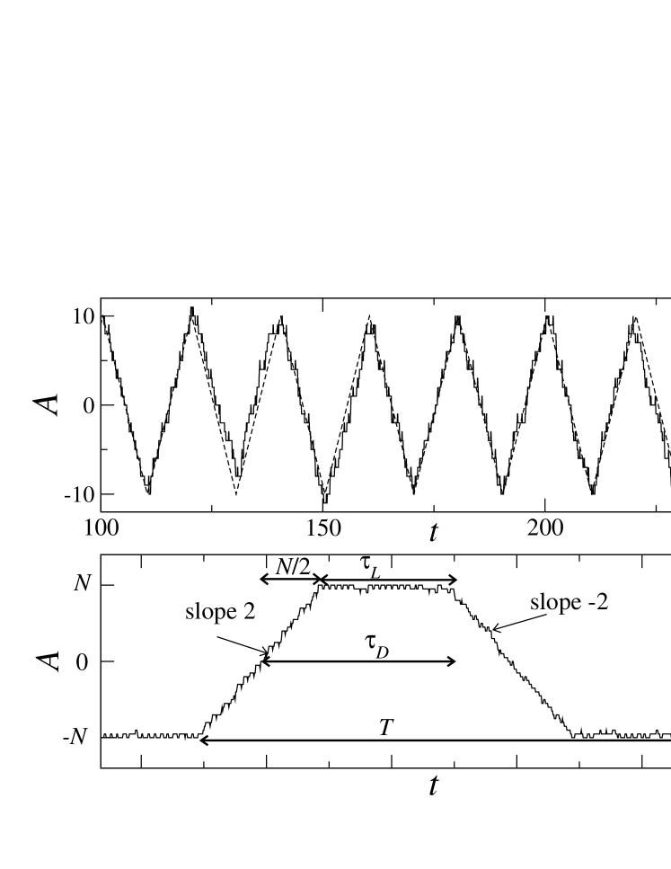
Figure 1: Unmodified dynamics of the system. Top: Comparison between simulations with $N=100$ and $\tau_{T}=0$ to Eq. (3). The delay is $\tau_{D}=5$, yielding a period of $20$ and an amplitude of $10$. Bottom: An example of $A(t)$ in the regime where servers go idle periodically.

Introducing a non-vanishing travel time $\tau_{T}$ has the same effect on $A(t)$ as increasing the delay time: it leads to the delay-differential equation

$$\frac{dA}{dt}(t+\tau_{T})=-2\mbox{sign}(A(t-\tau_{D})).$$ (5)

The solution is given by Eq. (3) with $t_{D}$ replaced by $t_{D}+t_{T}$.

The impact of idle servers – The case where oscillations become so strong that servers go idle periodically ($2\tau_{D}>N$) can be treated in a similar framework, for $t_{T}=0$: once the difference in queue lengths reaches the value $\pm N$, one queue ceases to process requests. Hence, the rate of requests at the other server drops from $2$ to $1$ – exactly the rate at which it keeps processing them. The queue length at the active server therefore stays constant for some time $\tau_{L}$. An example of the resulting curve can be seen in Fig. 1 (bottom). Starting from the time where $A(t)$ crosses the zero line, it will take a time $\tau_{D}$ for clients to realize that they are using the “wrong” server, so $\tau_{D}=\tau_{L}+N/2$, or $\tau_{L}=\tau_{D}-N/2$. The period $T$ of the oscillations is then $T=2\tau_{L}+2N=2\tau_{D}+N$, which is smaller than $4\tau_{D}$. Data throughput of the system drops from $2$ to $1+N/(2\tau_{D})$ (in units of $1/\tau_{P}$). All of this is again in good agreement with simulations.

The results above specify the system parameters for which oscillations affect throughput, and how strong the impact is. We now consider ways for the servers to reduce oscillations. Two methods suggest themselves: global disinformation from both servers and individual rejection by each server.

Global disinformation – If the servers have control over the information that clients receive on the servers’ status, they can intentionally make the information unreliable. Let us assume clients have a probability $p$ of receiving the wrong answer, and accordingly choose the “wrong” server. The update equations are:

$$\frac{dN_{1}}{dt} = 2[(1-p)\Theta(-A(t-\tau_{D}))+p\;\Theta(A(t-\tau_{D}))]-1;$$

$$\frac{dN_{2}}{dt} = 2[(1-p)\Theta(A(t-\tau_{D}))+p\;\Theta(-A(t-\tau_{D}))]-1,$$ (6)

leading to

$$\frac{dA}{dt}=-2(1-2p)\mbox{sign}(A(t-\tau_{D})).$$ (7)

This equation has the form of Eq. (2) with a prefactor of $1-2p$, and has a steady-state solution

$$A(t)=2\,\tau_{D}\,(1-2p)\mbox{tri}\left(\frac{t}{4\tau_{D}}+\phi\right),$$ (8)

for $p<1/2$. At $p=1/2$, no information is available: clients’ decisions are random, and queue lengths perform a random walk, whose fluctuations are not captured by the deterministic framework we are using. Even for values $p<1/2$, fluctuations may become larger than the typical amplitude of oscillations, and thus dominate the dynamics. For $p>1/2$, users migrate systematically from the less busy to the busier server, until one is idle much of the time, and the other has almost all clients in its queue.

The trade-off between reduced oscillations and increased fluctuations can be seen in Fig. 2. Rather than measuring the amplitude of oscillations, the root mean square $A_{rms}=\langle A^{2}\rangle^{1/2}$ of $A(t)$ is shown. For a pure triangle function of amplitude $a$, one gets $A_{rms}=a/\sqrt{3}$. For small $p$, the amplitude is reduced linearly; for larger $p$, fluctuations increase, dominating the dampened oscillations. When the amplitude of the undisturbed system is small, fluctuations have a large impact. As the amplitude of oscillations gets larger, the impact of fluctuations becomes smaller, and the value of $p$ where fluctuations dominate moves closer to $1/2$.

Under the influence of randomness, $A$ performs a biased random walk: let us assume that server $R_{2}$ is currently preferred. In each unit of time, $A/4$ increases by $1$ with probability $p^{2}$ (the two clients processed both go to $R_{1}$), stays constant with probability $p(1-p)$, and decreases by 1 with probability $(1-p)^{2}$ (both clients move from $R_{1}$ to $R_{2}$). To reproduce quantitatively the effects of fluctuations, one can numerically average $A^{2}$ over such a random walk that takes place in two phases: the first phase lasts until $A=0$ is reached; the second takes another $\tau_{D}$ steps until the direction of the bias is reversed. The probability distribution of $A$ at the beginning of the half-period has to be chosen self-consistently such that it is a mirror-image of the probability distribution at the end; the proper choice for $A/4$ is a Gaussian restricted to positive values with mean $(1-2p)\tau_{D}$ and variance $2p(1-p)\tau_{D}$. The numerical results are shown in Fig. 2; they agree well with values from the simulation. Note that in the above treatment, we neglected complications like multiple crossings of the $A=0$ line.

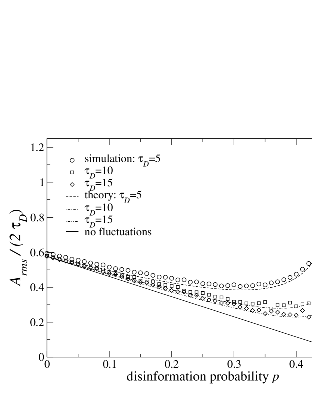
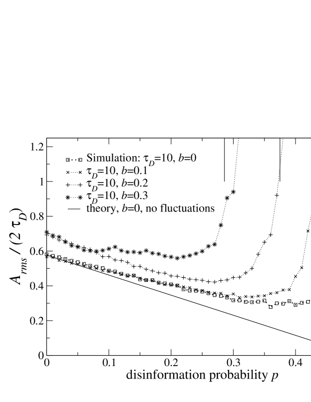
Figure 2: Top: Global disinformation – the $y$-axis shows the root mean square difference in queue lengths, rescaled by the amplitude of the undisturbed system. The theory for negligible fluctuations is given by Eq. (8); agreement with simulations becomes better as absolute amplitudes increase. The impact of fluctuations can be modeled using a discrete random walk.
Bottom: Adaptability – if a percentage $b$ of clients always chooses the same server, disinformation disrupts coordination for values $p\lesssim(1-2b)/(2-2b)$, indicated by vertical lines for several values of $b$.

Adaptability – Another aspect that determines what degree of disinformation should be chosen is adaptability of the system. The reason to have public information about the servers in the first place is to be able to compensate for changes in the environment: e.g., one server might change its data throughput due to hardware problems, or some clients might, for whatever reason, develop a strong preference for one of the servers. If the other agents can respond to these changes, global coordination remains good; if their ability to understand the situation is too distorted by disinformation, global efficiency suffers.

Let us assume that a fraction $b$ of agents decide to send their requests to server 1, regardless of the length of queues. Under global disinformation, out of the fraction $1-b$ that is left, another fraction $d$ will send their requests to the wrong server, and yet another fraction $d$ is needed to compensate for that. So a fraction $(1-b)(1-2d)$ is left to compensate for the action of the biased group, and the maximum level of disinformation that still leads to reasonable coordination is $p=(1-2b)/(2-2b)$ – larger levels lead to large differences in queue length, and finally to loss of data throughput by emptying a queue. That estimate is confirmed by simulations (see Fig. 2). Similar arguments hold if the preferences vary slowly compared to oscillation times. On the other hand, if the preferences of the biased agents oscillate in time with a period smaller than the delay time, they average out and have little effect on the dynamics.

A similar argument also applies if the servers have different capacity. Let us say $R_{1}$ has a processing time $\tau_{P1}$, whereas $R_{2}$ has $\tau_{P2}>\tau_{P1}$. A fraction $f=\tau_{P2}/(\tau_{P1}+\tau_{P2})>1/2$ of clients should choose $R_{1}$ – if $p$ is smaller than $1-f$, the queue of $R_{1}$ will not become empty; otherwise it will.

Individual rejection – Even if servers cannot influence the public information on queue status, they can influence the behavior of clients directly: they claim they are not capable of processing a request, and reject it – let us say, with a constant probability $r$. Compared to global disinformation, a new possibility arises that a request bounces back and forth several times between the servers, but that adds nothing new in principle: the fraction of requests that end up at the server that they tried at first is $(1-r)+r^{2}(1-r)+r^{4}(1-r)+\dots=1/(r+1)$, whereas a fraction $r/(r+1)$ will be processed at the other server. This is equivalent to setting $p=r/(1+r)$ in the “global disinformation” scheme, and gives equivalent results. Choosing $r$ close enough to $1$ reduces the amplitude of oscillations dramatically; however, each message is rejected a large number of times on average, generating large amounts of extra traffic.

Load-dependent rejection – Rather than setting a constant rejection rate, it seems intuitive to use a scheme of load-dependent rejection (LDR), in which $r_{i}$ depends on the current length of the queue. This is being considered for preventing the impact of single server overload in Ref. Braden et al. (1998). For example, let us consider the case where $r_{i}=cN_{i}$ if $cN_{i}<1$, and $1$ otherwise, with some appropriately chosen constant $c$. The analysis from the “indiviual rejection” section can be repeated with the additional slight complication of two different rejection rates $r_{1}$ and $r_{2}$. A fraction $(1-r_{1})/(1-r_{1}r_{2})$ of agents who initially try server 1 ends up being accepted by it, whereas a fraction $r_{1}(1-r_{2})/(1-r_{1}r_{2})$ finally winds up at server 2, and vice versa for clients who attempted $2$ first. Combining the resulting delay-differential equations for $N_{1}$ and $N_{2}$ into one for $A$, one obtains

$$\frac{dA}{dt}=\frac{2}{1-r_{1}r_{2}}(\Theta(-A(t-\tau_{D}))(1-2r_{1}+r_{1}r_{2})-\Theta(A(t-\tau_{D}))(1-2r_{2}+r_{1}r_{2})).$$ (9)

We can now substitute the load-dependent rates. We write them as follows: $r_{1}=\bar{r}+c^{\prime}A$, $r_{2}=\bar{r}-c^{\prime}A$, with $\bar{r}=(r_{1}+r_{2})/2$ and $c^{\prime}=c/2$.

For small amplitudes $A$ relative to the total number of players $N$, the deviation from $\bar{r}$ does not play a significant role, and it is $\bar{r}$ that determines behavior, yielding the same results as a constant rejection rate. For larger relative amplitudes, the oscillations are no longer pure triangle waves, but have a more curved tip. Figure 3 shows $A_{rms}$ for load-dependent rejection, compared to constant-rate rejection with $r=\bar{r}$. These nonlinear effects make LDR more efficient at suppressing oscillations, at least if $2\tau_{D}$ is not small compared to $N$. They also provide for a restoring force that suppresses fluctuations effectively. It follows that LDR is better at improving data throughput in parameter regimes where servers empty out, which is confirmed by simulations.

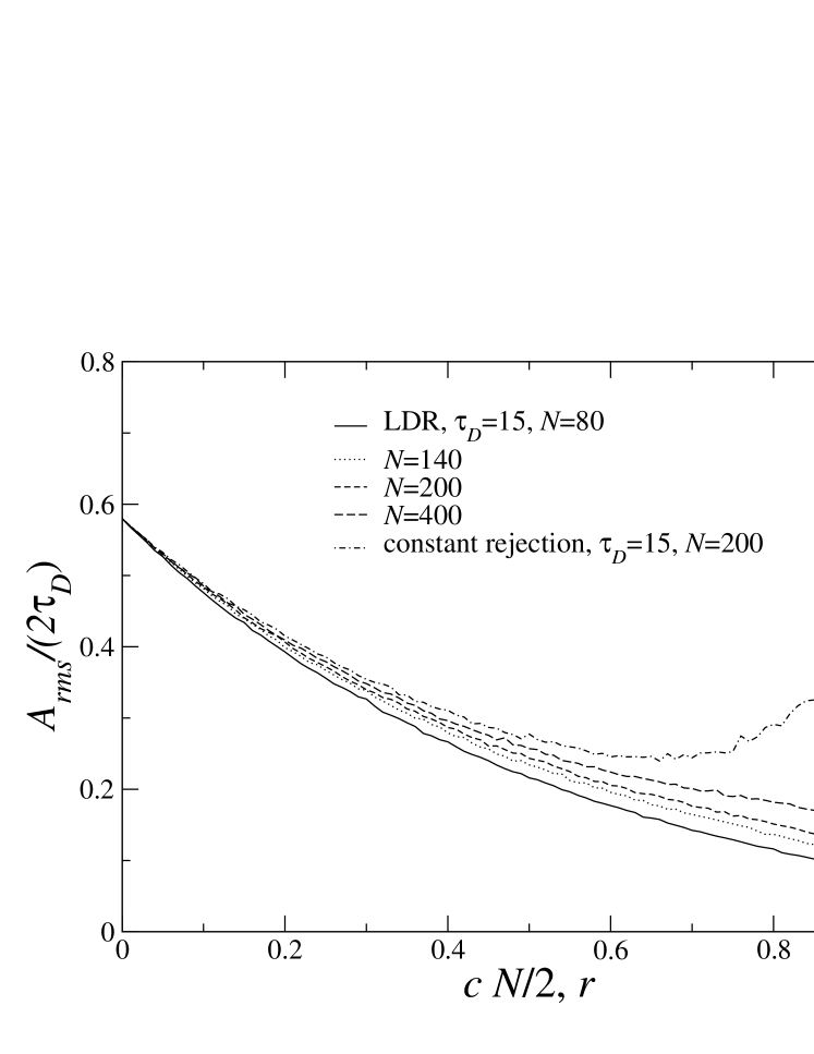
Figure 3: Load-dependent rejection: compared to rejection with a constant rate, LDR is more efficient at suppressing both oscillations and fluctuations. The former becomes more pronounced if $2\tau_{D}$ is not small compared to $N$.

We note one problem with LDR: if $c>2/N$, both servers have the maximal number $1/c<N/2$ clients in their queue most of the time, while the rest of clients are rejected with probability 1 from both servers. For effective operation, this means that the constant $c$ in LDR should chosen smaller than $2/N$, which requires knowledge of $N$.

Discussion – We have introduced a model for the coordination of clients’ requests for service from two equivalent servers, found the dependencies of the resulting oscillations on the parameters of the model, and determined when and how these oscillations decrease data throughput.

We have then suggested a number of server-side ways to dampen the oscillations, which involve purposely spreading wrong information about the state of the servers. All of these schemes can achieve an improvement, showing that the presence of faulty or incomplete information can be beneficial for coordination. The margins for improvement are higher in the regime of large numbers, when the amplitude is on the order of many tens or hundreds rather than a few individuals – in the latter case, increased fluctuations can outweigh the benefits of reduced oscillation. While some disinformation generally improves performance, monitoring of the average load and amplitude is necessary to choose the optimal degree of disinformation.

The basic ingredients of the server-client scenario (delayed public information and minority-game-like structure) appear in many circumstances. One can think of traffic guidance systems that recommend one of two alternative routes, stock buying recommendations in magazines, career recommendations by employment centers, and others. Exploring the impact of disinformation on these problems is certainly worthwhile.

References

- Smith (1904) A. Smith, An Inquiry into the Nature and Causes of the Wealth of Nations (Methuen and Co., Ltd, London, 1904).
- Challet and Zhang (1997) D. Challet and Y.-C. Zhang, Physica A 246, 407 (1997).
- Challet and Marsili (1999) D. Challet and M. Marsili, Phys. Rev. E 60, R6271 (1999).
- (4) Minority game homepage (with extensive bibliography), http://www.unifr.ch/econophysics/minority.
- Nakar and Hod (2002) E. Nakar and S. Hod (2002), cond-mat/0206056.
- Reents et al. (2001) G. Reents, R. Metzler, and W. Kinzel, Physica A 299, 253 (2001).
- Marsili and Challet (2000) M. Marsili and D. Challet (2000), cond-mat/0004376.
- Savit et al. (1999) R. Savit, R. Manuca, and R. Riolo, Phys. Rev. Lett. 82, 2203 (1999).
- Klein and Bar-Yam (2003) M. Klein and Y. Bar-Yam, Handling Resource Use Oscillation in Open Multi-Agent Systems. aAMAS Workshop (2003).
- Braden et al. (1998) B. Braden, D. Clark, et al., Recommendations on Queue Management and Congestion Avoidance in the Internet. Network Working Group (1998).