Flat histogram version of the pruned and enriched Rosenbluth method

Abstract

In this letter we present a flat histogram algorithm based on the pruned and enriched Rosenbluth method (PERM). This algorithm incorporates in a straightforward manner microcanonical reweighting techniques, leading to “flat histogram” sampling in the chosen parameter space. As an additional benefit, our algorithm is completely parameter free and, hence, easy to implement. We apply this algorithm to interacting self-avoiding walks (ISAW), the generic lattice model of polymer collapse.

Recently, there has been revived interest in flat histogram algorithms wang2001 , which strive to evenly sample configuration space with respect to a chosen parameterization, e.g. microcanonical energy. These algorithms are particular implementations of “umbrella sampling” torrie1977 , in which the configuration space is sampled according to a given probability distribution, the so-called “umbrella”. This umbrella distribution is generally chosen such that the whole configuration space of interest is accessible in one simulation. One major difficulty hereby is to find a suitable umbrella distribution.

There has also been an exciting development in stochastic growth algorithms, which are based on the Rosenbluth and Rosenbluth algorithm rosenbluth1955 . If this algorithm, which kinetically grows configurations, gets enhanced by cleverly chosen enrichment and pruning steps grassberger1997 , one obtains the pruned and enriched Rosenbluth method (PERM), a powerful algorithm for, e.g., simulation of the polymer collapse transition.

We present in this letter a new algorithm, flatPERM, which is a combination of these two types of algorithms, i.e. a flat histogram version of the pruned and enriched Rosenbluth method.

As opposed to earlier work in this direction bachmann2003 , in which an iterative scheme similar to the multicanonical algorithm berg1991 was used, we utilize the self-tuning capabilities of PERM directly. This leads to a considerable simplification of the algorithm.

While flatPERM includes umbrella sampling ideas, it is stricly speaking not a multicanonical method, as multicanonical sampling conventionally describes a particular iterative version of adaptive umbrella sampling, in which first an umbrella distribution is obtained iteratively and then a final simulation is performed with a fixed umbrella distribution.

This letter is structured as follows: we first give a pedagogical introduction to PERM, which will then allow us to introduce flatPERM as a seemingly trivial extension. As an application, we present simulations of interacting self-avoiding walks (ISAW) on the square lattice and the simple cubic lattice. We conclude with a description of further applications.

We will consider a rather abstract setting of configurations with a certain size $n$, which is parameterized with an additional variable $m$. In general, one can even consider a set of variables $m_{i}$, but for pedagogical reasons we shall in this paper restrict ourselves to the case of $m$ corresponding to an energy $E=\epsilon m$. Both $n$ and $m$ are assumed to have non-negative integer values. Moreover, we will need the notion of “atmosphere” of a configuration, which is the number $a$ of different ways to continue to grow this configuration, and is also a non-negative integer.

While it is useful to present the algorithm in such an abstract setting, it may help the reader to keep the application to interacting self-avoiding walks (ISAW) on a regular lattice in mind. In this case, the size of the configuration is the number of steps of the walk, the energy is the number of non-consecutive nearest-neighbor bonds, and the atmosphere is the number of non-occupied sites around the endpoint of the walk. If all the sites around the endpoint are occupied, then the atmosphere is zero and the walk cannot be continued.

The basis of the algorithm is the Rosenbluth and Rosenbluth algorithm, a stochastic growth algorithm in which the configurations of interest are grown from scratch. The growth is kinetic, which is to say that each growth step is selected at random from all possible growth steps. Thus, if there are $a$ possible ways of growth, one selects one of them with probability $p=1/a$. As this number generally changes during the growth process, different configurations are thus generated with different probabilities, and one needs to resort to reweighting techniques.

It is advantageous to view this algorithm as approximate counting, in which case the weights of the configurations serve as estimates of the number of configurations. To understand this point of view, imagine that we were to perform a complete enumeration of the configuration space. Doing this requires that at each growth step we would have to choose all the possible continuations and count them each with equal weight. If we now select fewer configurations, we have to change the weight of these configurations accordingly, in order to correct for missing out on some configurations. Thus, if we choose one growth step out of $a$ possible ones, we replace $a$ configurations with equal weight by one “representative” configuration with $a$-fold weight. In this way, the weight of each grown configuration is a direct estimate of the total number of configurations.

Let the atmosphere $a_{n}=a(\varphi_{n})$ be the number of distinct ways in which a configuration $\varphi_{n}$ of size $n$ can be extended. Then, the weight associated with a configuration of size $n$ is the product of all the atmospheres $a_{k}$ encountered while growing this configuration, i.e.

$$W=\prod_{k=0}^{n-1}a_{k}\;.$$ (1)

After having started $S$ growth chains, an estimator $C_{n}^{est}$ for the total number of configurations $C_{n}$ (the “infinite-temperature” partition function, in which all configurations appear with equal weight $1$) is given by the mean over all generated samples $\varphi_{n}^{(i)}$ of size $n$ with respective weights $W_{n}^{(i)}$, i.e.

$$C_{n}^{est}=\langle W\rangle_{n}=\frac{1}{S}\sum_{i}W_{n}^{(i)}\;.$$ (2)

Here, the mean is taken with respect to the total number of growth chains $S$, and not the number of configurations which actually reach size $n$. Configurations which get trapped before they reach size $n$ appear in this sum with weight zero.

The problem with the Rosenbluth and Rosenbluth algorithm is two-fold. Firstly, the weights can vary widely in magnitude, so that the mean can get to be dominated by very few samples with very large weight. Secondly, regularly occurring trapping events, i.e. generation of configurations with zero atmosphere, can lead to exponential “attrition”, i.e. exponentially strong suppression of configurations of large sizes.

To overcome both of these problems, enrichment and pruning steps have been added to this algorithm, leading to the pruned and enriched Rosenbluth method (PERM) grassberger1997 . The basic idea is that one wishes to suppress fluctuations in the weights $W_{n}^{(i)}$, as these should on average be equal to $C_{n}$. Therefore, if the weight is too large, one enriches, i.e. one makes copies of the configuration and reduces the weight accordingly. On the other hand, if the weight is too small, one prunes probabilistically, and, in case the pruning is unsuccessful, continues growing with appropriately increased weight. Note that $S$, and therefore the expression (2) for the estimate $C_{n}^{est}$, is not changed by either enriching or pruning steps.

We need to specify enrichment and pruning criteria as well as the actual enrichment and pruning processes. While the idea of PERM itself is straightforward, there is now a lot of freedom in the precise choice of the pruning and the enrichment steps. The “art” of making PERM perform efficiently is based to a large extent on a suitable choice of these steps. Distilling our own experience with PERM, we present here what we believe to be an efficient, and, most importantly, parameter free version.

In contrast to other expositions of PERM (e.g. hsu2003 ), we propose to prune or enrich constantly, to enable larger exploration of the configuration space (the motivation will become clear once flatPERM is introduced below). Define $r$ as the ratio of weight and estimated number of configurations, $r=W_{n}^{(i)}/C_{n}^{est}$. Then we enrich if $r>1$ and prune if $r<1$. Moreover, the actual pruning and enrichment steps are chosen such that the weights are set as closely as possible to $C_{n}^{est}$ to minimize fluctuations:

• $r>1$ $\rightarrow$ enrichment step:
  make $c=\min(\lfloor r\rfloor,a_{n})$ distinct copies, each with weight $\frac{1}{c}W_{n}^{(i)}$ (as in nPERM hsu2003a ).

• $r<1$ $\rightarrow$ pruning step:
  continue growing with probability $r$ and weight $C_{n}^{est}$ (i.e. prune with probability $1-r$).

Note that we perform pruning and enrichment after the configuration has been included in the calculation of $C_{n}^{est}$ and is used for weights during the next growth step. Initially, the estimates $C_{n}^{est}$ can of course be grossly wrong, as the algorithm knows nothing about the system it is simulating. However, even if initially “wrong” estimates are used for pruning and enrichment, in all applications considered the algorithm can be seen to converge to the true values. It is, in a sense, self-tuning.

At this point it is now straight-forward to change PERM to a thermal ensemble with inverse temperature $\beta=1/k_{B}T$ and energy $E=\epsilon m$ by multiplying the weight with the appropriate Boltzmann factor $\exp(-\beta E)$, which leads to an estimate of the partition function $Z_{n}(\beta)$ of the form

$$Z_{n}^{est}(\beta)=\langle W\exp(-\beta E)\rangle_{n}\;.$$ (3)

The pruning and enrichment procedures are changed accordingly, replacing $W$ by $W\exp(-\beta E)$ and $C_{n}^{est}$ by $Z_{n}^{est}(\beta)$, and using $r=W_{n}^{(i)}\exp(-\beta E_{m}^{(i)})/Z_{n}^{est}(\beta)$. (It is in this setting that PERM is usually described.)

Alternatively, however, it is also possible to consider microcanonical estimators for the total number $C_{n,m}$ of configurations of size $n$ with energy $m$ (i.e. the “density of states”). An appropriate estimator $C_{n,m}^{est}$ is then given by the mean over all generated samples $\varphi_{n,m}^{(i)}$ of size $n$ and energy $m$ with respective weights $W_{n,m}^{(i)}$, i.e.

$$C_{n,m}^{est}=\langle W\rangle_{n,m}=\frac{1}{S}\sum_{i}W_{n,m}^{(i)}\;.$$ (4)

Again, the mean is taken with respect to the total number of growth chains $S$, and not the number of configurations $S_{n,m}$ which actually reach a configuration of size $n$ and energy $m$. The pruning and enrichment procedures are also changed accordingly, replacing $C_{n}$ by $C_{n,m}$ and using $r=W_{n,m}^{(i)}/C_{n,m}^{est}$.

At this point it is worth pointing out that the pruning and enrichment criterion for PERM leads to a roughly constant number of samples being generated at each size $n$ for PERM. In fact, one can motivate the given pruning and enrichment criteria by stipulating that one wishes to have a roughly constant number of samples, as this leads to the algorithm performing an unbiased random walk in the configuration size. Correspondingly, in the flat-energy version the algorithm performs an unbiased random walk in both size and energy of the configuration, and we obtain a roughly constant number of samples for each size $n$ and energy $m$.

It is because of the fact that the number of samples is roughly constant in each histogram entry, that this algorithm can be seen as a “flat histogram” algorithm, which we consequently call flatPERM. In hindsight in becomes clear that PERM itself can be seen as a flat histogram algorithm, at it creates a roughly flat histogram in size $n$. Recognizing this led us to the formulation of this algorithm in the first place.

At this point we return to our discussion of the pruning and enrichment strategies. For PERM it may be more advantageous to allow for a high diffusivity along the size $n$. This is done by minimizing pruning and enrichment, i.e. at the cost of allowing larger weight fluctuations. For flatPERM on the other hand we need to achieve diffusive behavior also with respect to the energy variable $m$. Precisely this is achieved by allowing for much enrichment (and thus necessarily also pruning), as each set of configurations enriched at size $n$ will contribute to a range of different energies $m$ at size $n+1$.

Even though we view flatPERM as a flat histogram algorithm, we have not yet explicitly conditioned the pruning and enrichment with respect to the local number of samples $S_{n,m}$ created at each size $n$ and energy $m$. This can be done by multiplying $r$ by $S/S_{n,m}$, as this enhances enrichment if $S_{n,m}<S$, i.e. when there are too few samples, and vice versa.

One general problem with PERM is that enrichment generates large correlation between samples, so that it would be useful to replace the number $S_{n,m}$ of samples by a number $S_{n,m}^{eff}$ of effectively independent samples, thereby taking account of some autocorrelation time. This can be done heuristically by considering the average number of independent growth steps in a configuration. If the last enrichment has occurred at size $n_{enr}$, then a configuration of size $n$ and energy $m$ has $n_{ind}=n-n_{enr}$ independent steps. The frequency of independent steps in a configuration is $w_{n,m}^{(i)}=n_{ind}/n$. We thus use

$$r=\frac{S}{S_{n,m}^{eff}}\frac{W_{n,m}^{(i)}}{C_{n,m}^{est}}\quad\mbox{with}\quad S_{n,m}^{eff}=\sum_{i}w_{n,m}^{(i)}$$ (5)

for the pruning and enrichment criterion in our algorithm.

Now that one has a flat histogram method of PERM for the whole range of energies, one can easily modify the algorithm further to sample only a selected range by dividing $r$ by a “profile shape” $f_{n,m}$, leading to pruning whenever $f_{n,m}$ is close to zero. This is advantageous if one only wants to explore a restricted region of parameter space.

Even though the algorithm described thus far is free of parameters, there is a technical problem due to the fact that initial weights are grossly wrong, which can lead to overflow problems. This can easily be overcome by initially restricting the maximal size of grown configurations, e.g. by limiting the maximal size by the number of started growth chains,

$$n<cS\;.$$ (6)

The relevant number of growth chains at size $n$ is thus reduced to $S-n/c$. For ISAW we find that a choice of delay of $c\approx 10$ is sufficient.

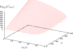
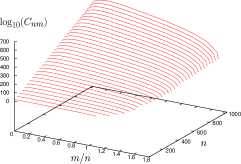
Figure 1: Logarithm of the number of configurations $C_{n,m}$ versus internal energy $m/n$ and length $n$ for ISAW on the square lattice (above) and simple cubic lattice (below).

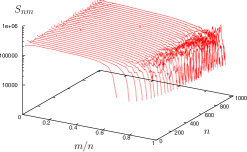
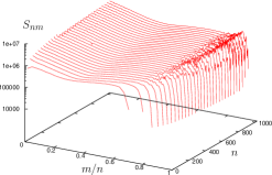
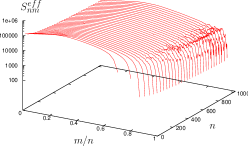
Figure 2: Number of generated samples versus internal energy $m/n$ and length $n$ for ISAW on square lattice. The top graph shows the number of samples $S_{n,m}$ for a simulation in which a flat histogram for $S_{n,m}$ was created, whereas the middle and bottom graphs show the number of samples $S_{n,m}$ and the effective number of samples $S_{n,m}^{eff}$, respectively, for a simulation in which a flat histogram for $S_{n,m}^{eff}$ was created.

Averages of observables $Q$ defined on the set of configurations can now be obtained by storing weighted sums of these observables, from which one obtains

$$Q_{n,m}^{est}=\frac{\langle QW\rangle_{n,m}}{\langle W\rangle_{n,m}}=\frac{\sum_{i}Q_{n,m}^{(i)}W_{n,m}^{(i)}}{\sum_{i}W_{n,m}^{(i)}}\;.$$ (7)

These can then be used for subsequent evaluations. For instance, the expectation value of $Q$ in the canonical ensemble at a given temperature $\beta$ can now be computed via

$$Q_{n}^{est}(\beta)=\frac{\sum_{m}Q_{n,m}^{est}C_{n,m}^{est}\exp(-\beta E_{m})}{\sum_{m}C_{n,m}^{est}\exp(-\beta E_{m})}\;.$$ (8)

We have implemented this algorithm for interacting self-avoiding walks on the square and simple cubic lattice. In both two and three dimensions, we have simulated walks up to length $n=1024$. Figures 1 and 2 clearly show the strength of the method. Figure 1 shows the number of configurations $C_{n,m}$, which vary over several hundred orders of magnitude. This range would have been inaccessible during one simulation with any canonical method. As an aside, we note that we had to rescale weights during the run to avoid overflow berg2003 . Additionally, we chose a delay of $c=10$ to stabilize the algorithm.

As can clearly be seen in Figure 2, the number of samples generated is roughly constant, irrespective of whether one flattens with respect to $S_{n,m}$ (top graph) or $S_{n,m}^{eff}$ (middle and bottom graphs). Only results for the square lattice are shown, as we find the same behavior for the simple cubic lattice. Using $S_{n,m}^{eff}$ for the flatness criterion leads moreover to an increased sampling of walks with very few and very many interactions, thus overcoming the usual difficulty of obtaining configurations with a large number of interactions. (The largest energy state gets repeatedly sampled in simulations in both dimensions.)

Figure 3: Normalized fluctuations $\sigma^{2}(m)/n$ versus inverse temperature $\beta=1/k_{B}T$ for ISAW on the square lattice (above) and the simple cubic lattice (below) at lengths 64, 128, 256, 512, and 1024. The curves for larger lengths are more highly peaked. The vertical lines denote the expected transition temperature at infinite length.

Once the simulations have been completed, thermodynamic quantities of interest can easily be computed. As an example, the specific heat curves $C_{n}=k_{B}(\beta\epsilon)^{2}\sigma^{2}(m)/n$ near the transition temperature are shown for both systems in Figure 3.

We have also tested our algorithm on the HP model dill1985 , which is a toy model for proteins. It consists of a self-avoiding walk with two types of monomers along the sites visited by the walk, which are either hydrophobic (type H) or polar (type P). One considers monomer-specific interactions, mimicking the interaction with a polar solvent such as water. The interaction strengths are thus chosen such that HH-contacts are favored, e.g. by choosing $\epsilon_{HH}=-1$ and $\epsilon_{HP}=\epsilon_{PP}=0$. The central question is to determine the density of states (and to find the ground state with lowest energy) for a given sequence of monomers. For various sequences taken from the literature we have confirmed previous density of states calculations and obtained identical ground state energies. The sequences we considered had $n=58$ steps ($3$ dimensions, $E_{min}=-44$) and $n=85$ steps ($2$ dimensions, $E_{min}=-53$) from hsu2003 , and $n=80$ steps ($3$ dimensions, $E_{min}=-98$) from frauenkron1998 . We studied also a particularly difficult sequence with $n=88$ steps ($3$ dimensions, $E_{min}=-73$) from beutler1996 , but the lowest energy we obtained was $E=-69$. However, in this case no lower energy has been found with any other PERM implementation either, see hsu2003 .

To summarize, we have presented a new algorithm, flatPERM, which is a flat histogram version of a stochastic growth algorithm. This algorithm can in principle be applied to any statistical mechanical system for which configurations can be grown in a well-defined manner. Next to the presented applications of linear polymers, this algorithm can be applied to more complicated systems, such as lattice models of branched polymers rechnitzer2004 . Extensions to models with two energy parameters are in preparation, e.g. to the problem of adsorbing interacting polymers owczarek2004 or an extended Domb-Joyce model of polymer collapse krawczyk2004 .

The authors thank Andrew Rechnitzer and Aleks Owczarek for helpful discussions, Peter Grassberger for pointing out an incorrect formula, the referees for helpful comments, and the DFG for financial support.

References

- (1) F. Wang and D. P. Landau, Phys. Rev. Lett. 86 2050 (2001)
- (2) G. M. Torrie and J. P. Valleau, J. Comput. Phys. 23 187 (1977)
- (3) M. N. Rosenbluth and A. W. Rosenbluth, J. Chem. Phys. 23 356 (1955)
- (4) P. Grassberger, Phys. Rev E 56 3682 (1997)
- (5) M. Bachmann and W. Janke, Phys. Rev. Lett. 91 208105 (2003)
- (6) B. A. Berg and T. Neuhaus, Phys. Lett. B 267 249 (1991)
- (7) H.-P. Hsu and V. Mehra and W. Nadler and P. Grassberger, J. Chem. Phys. 118 444 (2003)
- (8) H.-P. Hsu and V. Mehra and W. Nadler and P. Grassberger, Phys. Rev. E 68 21113 (2003)
- (9) An alternative is to use logarithmic coding, see e.g. eqn. (20) in B. A. Berg, Comp. Phys. Commun. 153 397 (2003)
- (10) K. A. Dill, Biochemistry 24 1501 (1985)
- (11) H. Frauenkron and U. Bastolla and E. Gerstner and P. Grassberger and W. Nadler, Phys. Rev. Lett. 80 3149 (1998)
- (12) T.C. Beutler and K.A. Dill, Protein Sci. 5 147 (1996)
- (13) A. Rechnitzer and E. Janse van Rensburg and T. Prellberg, in preparation
- (14) A. L. Owczarek and A. Rechnitzer and J. Krawczyk and T. Prellberg, in preparation
- (15) J. Krawczyk and T. Prellberg and A. Rechnitzer and A. L. Owczarek, in preparation