Temperature Dependence of the Hydrophobic Hydration and Interaction of Simple Solutes: An Examination of Five Popular Water Models

Abstract

We examine five different popular rigid water models (SPC, SPCE, TIP3P, TIP4P and TIP5P) using molecular dynamics simulations in order to investigate the hydrophobic hydration and interaction of apolar Lennard-Jones solutes as a function of temperature in the range between $275\;\mbox{K}$ and $375\;\mbox{K}$ along the $0.1\;\mbox{MPa}$ isobar. For all investigated models and state points we calculate the excess chemical potential for the noble gases and Methane employing the Widom particle insertion technique. All water models exhibit too small hydration entropies, but show a clear hierarchy. TIP3P shows poorest agreement with experiment whereas TIP5P is closest to the experimental data at lower temperatures and SPCE is closest at higher temperatures. As a first approximation, this behaviour can be rationalised as a temperature-shift with respect to the solvation behaviour found in real water. A rescaling procedure inspired by information theory model of Hummer et al. (Chem.Phys. 258, 349-370 (2000)) suggests that the different solubility curves for the different models and real water can be largely explained on the basis of the different density curves at constant pressure. In addition, the models that give a good representation of the water structure at ambient conditions (TIP5P, SPCE and TIP4P) show considerably better agreement with the experimental data than the ones which exhibit less structured O-O correlation functions (SPC and TIP3P). In the second part of the paper we calculate the hydrophobic interaction between Xenon particles directly from a series of 60 ns simulation runs. We find that the temperature dependence of the association is to a large extent related to the strength of the solvation entropy. Nevertheless, differences between the models seem to require a more detailed molecular picture. The TIP5P model shows by far the strongest temperature dependence. The suggested density-rescaling is also applied to the chemical potential in the Xenon-Xenon contact-pair configuration, indicating the presence of a temperature where the hydrophobic interaction turns into purely repulsive. The predicted association for Xenon in real water suggest the presence a strong variation with temperature, comparable to the behaviour found for TIP5P water. Comparing different water models and experimental data we conclude that a proper description of density effects is an important requirement for a water model to account correctly for the correct description of the hydrophobic effects. A water model exhibiting a density maximum at the correct temperature is desirable.

I INTRODUCTION

Nonpolar solutes show a strong tendency to aggregate when dissolved in water due to the relatively strong water-water interaction in comparison to the weak solute-water interaction Ben-Naim (1980); Kauzmann (1959); Ben-Naim and Wilf (1979). However, in addition to such energetical considerations the hydration entropy of small simple solutes is found to be negative, which is usually explained as increased ordering of the molecules in the hydration shell Privalov and Gill (1988); Haymet et al. (1996). This is the characteristic feature of the so called hydrophobic hydration of small apolar particles Pierotti (1976); Pratt and Chandler (1977). As a consequence, with increasing temperature the association of hydrophobic particles is found to be enhanced in order to minimise the solvation entropy penalty Smith et al. (1992); Smith and Haymet (1993). This entropy-driven association process is usually referred to as hydrophobic interaction and has been subject of numerous simulation studies Geiger et al. (1979); Zichi and Rossky (1985); Smith et al. (1992); Smith and Haymet (1993); Pearlman (1993); van Belle and Wodak (1993); Dang (1994); Forsman and Jönsson (1994); Lüdemann et al. (1996); Skipper et al. (1996); Young and Brooks III. (1997); Hummer et al. (1996); Lüdemann et al. (1997); Rick and Berne (1997); Hummer (2001); Shimizu and Chan (2000); Rick (2000); Shimizu and Chan (2001); Ghosh et al. (2001, 2002).

Hydrophobic effects are considered to play an important role concerning protein stability and other self assembly phenomena Tanford (1980); Privalov and Gill (1988); Huang and Chandler (2000). The strength of hydrophobic interactions, however, might as well determine largely the temperature-range where the protein remains physiologically functional before thermal unfolding takes place. In addition, the weakening of hydrophobic interactions at lower temperatures is presumably of importance for the understanding of the cold denaturation of proteins Privalov (1990); Tsai et al. (2002); Kumar et al. (2003). This is probably of particular importance for systems that show an entropy driven configurational “folding” transition such as the “hydrophobic” collapse of polymeric elastin Urry (1993); Darwin et al. (2001) and small tropoelastin-like oligo-peptides Reiersen et al. (1998) around $300\,\mbox{K}-330\,\mbox{K}$. The present status of conceptual understanding of hydrophobic hydration and hydrophobic interaction has been reviewed recently by Pratt Pratt (2003) and Southall et al. Southall et al. (2002), whereas Smith and Haymet Smith and Haymet (2003) give a tutorial overview over the currently available computational methods.

Recent methodological improvements in simulation techniques, such as the “parallel tempering” approach (or “replica exchange molecular dynamics”) give rise to the possibility of explicitly studying the thermal folding/unfolding transition of solvated proteins Gnanakaran et al. (2003); Sanbonmatsu and Garcia (2002). Molecular dynamics simulations of proteins in aqueous solution, however, still largely depend on the use of simple model potentials for water. Therefore it might be interesting to compare different popular rigid water models with respect to hydrophobic interactions and to show how their strengths might be related to the behaviour of other known thermodynamical and structural properties of the model liquids. For this purpose we employ the three center point charge models proposed by the Berendsen group (SPC Berendsen et al. (1981) and SPCE Berendsen et al. (1987)) as well as three candidates representing the TIP-family of water models according to Jorgensens group: The three center TIP3P and four center TIP4P Jorgensen et al. (1983), as well as the recently proposed five center TIP5P model Mahoney and Jorgensen (2000).

The most simple and as well most often studied hydrophobic model system in this context is, of course, hydrophobic Lennard-Jones particles dissolved in water Pratt and Pohorille (2002). The outline of the paper is therefore the following.

First we would like to examine the the performance of the five different models with respect to the hydrophobic hydration behaviour as a function of temperature with a focus on the physiologically important temperature range between $275\,\mbox{K}$ and $375\,\mbox{K}$. This is done a in the spirit of the paper by Guillot and Guissani Guillot and Guissani (1993) where we calculate the chemical potentials and solvation entropies for Lennard Jones particles representing the noble gases and Methane and compare them with experimental data. Simulation runs of $20\,\mbox{ns}$ allow an accurate determination of the excess chemical potential using the Widom particle insertion method.

In the second part of the paper we study the association behaviour of hydrophobic particles (only Xenon) as a function of temperature for all five water models by conducting long ($60\,\mbox{ns}$) MD simulation runs of solutions of the hydrophobic particles in water, as suggested recently by the work of Ghosh et al. Ghosh et al. (2001, 2002). The potential of mean force (PMF) between the hydrophobic particles can then be obtained directly from the pair distribution functions. Thus we are able to calculate the hydrophobic interaction for the different models as a function of temperature.

A very recent study on lattice models by Widom et al. Widom et al. (2003) suggests a linear relationship between the strength of the hydrophobic hydration and and the hydrophobic pair interaction. Therefore it might also be interesting to provide accurate data for both on a set of realistic water models.

II METHODS

II.1 MD Simulation details

Model	$\sigma/\mbox{\AA}$	$\epsilon\,k_{B}^{-1}/\mbox{K}$	$q/\mbox{e}$
SPC	$3.1656$(O)	$78.2$(O)	$0.41$(H)
SPCE	$3.1656$(O)	$78.2$(O)	$0.4238$(H)
TIP3P	$3.1506$(O)	$76.58$(O)	$0.417$(H)
TIP4P	$3.1536$(O)	$78.08$(O)	$0.52$(H)
TIP5P	$3.12$(O)	$80.56$(O)	$0.241$(H)
Ne	$3.035$	$18.6$	$0$
Ar	$3.415$	$125.0$	$0$
Kr	$3.675$	$169.0$	$0$
Xe	$3.975$	$214.7$	$0$
$\mbox{CH}_{4}$	$3.730$	$147.5$	$0$

Table 1: Lennard-Jones potential parameters and partial charges describing the water-water and solute-solute pair interactions. The solute-water cross parameters are deduced from the Lorentz-Berthelot mixing rules: $\sigma_{ij}\!=\!\left(\sigma_{ii}+\sigma_{jj}\right)/2$, $\epsilon_{ij}\!=\!\sqrt{\epsilon_{ii}\epsilon_{jj}}$. For further information on the geometry of the water models we refer to the original references Berendsen et al. (1981, 1987); Jorgensen et al. (1983); Mahoney and Jorgensen (2000). The solute-solute-parameters were taken from Refs. Hirschfelder et al. (1954); Guillot and Guissani (1993).

We employ molecular dynamics (MD) simulations in the NPT ensemble using the Nosé-Hoover thermostat Nosé (1984); Hoover (1985) and the Rahman-Parinello barostat M. Parrinello (1981); Nosé and Klein (1983) with coupling times $\tau_{T}\!=\!1.5\,\mbox{ps}$ and $\tau_{p}\!=\!2.5\,\mbox{ps}$ (assuming the isothermal compressibility to be $\chi_{T}\!=\!4.5\;10^{-5}\,\mbox{bar}^{-1}$), respectively. The electrostatic interactions are treated in the “full potential” approach by the smooth particle mesh Ewald summation Essmann et al. (1995) with a real space cutoff of $0.9\,\mbox{nm}$ and a mesh spacing of approximately $0.12\,\mbox{nm}$ and 4th order interpolation. The Ewald convergence factor $\alpha$ was set to $3.38\,\mbox{nm}^{-1}$ (corresponding to a relative accuracy of the Ewald sum of $10^{-5}$). A $2.0\,\mbox{fs}$ timestep was used for all simulations and the constraints were solved using the SETTLE procedure Miyamoto and Kollman (1992). All simulations reported here were carried out using the GROMACS 3.1 program Lindahl et al. (2001); van der Spoel et al. (2001). Statistical errors in the analysis were computed using the method of Flyvbjerg and Petersen Flyvbjerg and Petersen (1989). For all reported systems and different statepoints initial equilibration runs of $1\,\mbox{ns}$ length were performed using the Berendsen weak coupling scheme for pressure and temperature control $\tau_{T}\!=\!\tau_{p}\!=\!0.5\,\mbox{ps}$ Berendsen et al. (1984).

In order to determine the excess chemical potential of the hydrophobic particles we performed a series of simulations generally using 256 water molecules for all five different water models SPC, SPCE, TIP3P, TIP4P and TIP5P (model parameters are given in Table 1). However, the excess chemical potential is known to be sensitive to finite size effects Siepmann et al. (1992). In order to estimate this influence, we additionally carried out simulations containing 500 and 864 water molecules but only for the SPCE model. All model systems were simulated at five different temperatures $275\,\mbox{K}$, $300\,\mbox{K}$, $325\,\mbox{K}$, $350\,\mbox{K}$ and $375\,\mbox{K}$ at a pressure of $0.1\,\mbox{MPa}$. Each of these simulations extended to $20\,\mbox{ns}$ and $2\times 10^{4}$ configurations were stored for further analysis. To determine the hydrophobic interaction between Xenon particles (for the model parameters see Table 1) we use MD simulations containing 500 water molecules and 8 Xenon particles employing the same simulation parameters outlined above. Again, the five different water model systems are studied at $275\,\mbox{K}$, $300\,\mbox{K}$, $325\,\mbox{K}$, $350\,\mbox{K}$ and $375\,\mbox{K}$ at a pressure of $0.1\,\mbox{MPa}$. Here, runs over $60\,\mbox{ns}$ were conducted, while storing $7.5\times 10^{4}$ configurations for further analysis. The simulations protocols showing the obtained densities and average potential energies are given in Table 2.

Model	$T/\mbox{K}$	$\left<\rho\right>/\mbox{kg}\,\mbox{m}^{-3}$	$\left<E\right>/\mbox{kJ}\,\mbox{mol}^{-1}$	$\left<\rho\right>/\mbox{kg}\,\mbox{m}^{-3}$	$\left<E\right>/\mbox{kJ}\,\mbox{mol}^{-1}$
SPC	$275$	$993.3\pm 0.2$	$-43.005\pm 0.003$	$1070.0\pm 0.1$	$-42.470\pm 0.001$
	$300$	$977.1\pm 0.1$	$-41.534\pm 0.002$	$1050.2\pm 0.1$	$-40.951\pm 0.001$
	$325$	$956.7\pm 0.1$	$-40.096\pm 0.001$	$1026.5\pm 0.1$	$-39.472\pm 0.001$
	$350$	$933.8\pm 0.1$	$-38.687\pm 0.002$	$999.5\pm 0.1$	$-38.019\pm 0.001$
	$375$	$907.8\pm 0.1$	$-37.277\pm 0.003$	$969.2\pm 0.1$	$-36.571\pm 0.001$
SPCE	$275$	$1009.5\pm 0.2$	$-48.148\pm 0.004$	$1089.9\pm 0.1$	$-47.594\pm 0.003$
	$300$	$998.6\pm 0.2$	$-46.572\pm 0.002$	$1076.1\pm 0.1$	$-45.968\pm 0.001$
	$325$	$983.8\pm 0.1$	$-45.066\pm 0.001$	$1057.5\pm 0.1$	$-44.408\pm 0.002$
	$350$	$965.3\pm 0.2$	$-43.598\pm 0.002$	$1035.7\pm 0.1$	$-42.897\pm 0.001$
	$375$	$944.3\pm 0.2$	$-42.154\pm 0.002$	$1010.2\pm 0.1$	$-41.405\pm 0.002$
SPCE (500 Mol.)	$275$	$1009.0\pm 0.1$	$-48.147\pm 0.003$
	$300$	$998.4\pm 0.1$	$-46.576\pm 0.001$
	$325$	$983.3\pm 0.1$	$-45.062\pm 0.001$
	$350$	$964.9\pm 0.1$	$-43.589\pm 0.001$
	$375$	$943.8\pm 0.1$	$-42.142\pm 0.002$
SPCE (864 Mol.)	$275$	$1009.0\pm 0.1$	$-48.152\pm 0.002$
	$300$	$998.2\pm 0.1$	$-46.577\pm 0.001$
	$325$	$983.3\pm 0.1$	$-45.066\pm 0.002$
	$350$	$964.8\pm 0.1$	$-43.592\pm 0.001$
	$375$	$943.6\pm 0.1$	$-42.149\pm 0.001$
TIP3P	$275$	$1005.2\pm 0.1$	$-41.300\pm 0.002$	$1079.8\pm 0.1$	$-40.753\pm 0.001$
	$300$	$984.6\pm 0.1$	$-39.921\pm 0.001$	$1055.8\pm 0.0$	$-39.329\pm 0.001$
	$325$	$960.9\pm 0.1$	$-38.565\pm 0.002$	$1028.4\pm 0.0$	$-37.937\pm 0.001$
	$350$	$934.6\pm 0.2$	$-37.229\pm 0.002$	$997.7\pm 0.1$	$-36.560\pm 0.001$
	$375$	$905.4\pm 0.2$	$-35.888\pm 0.002$	$963.9\pm 0.1$	$-35.182\pm 0.001$
TIP4P	$275$	$1005.3\pm 0.1$	$-42.839\pm 0.003$	$1089.0\pm 0.1$	$-42.957\pm 0.002$
	$300$	$993.5\pm 0.1$	$-41.237\pm 0.003$	$1075.2\pm 0.1$	$-41.249\pm 0.001$
	$325$	$976.5\pm 0.1$	$-39.697\pm 0.002$	$1055.0\pm 0.1$	$-39.624\pm 0.001$
	$350$	$955.1\pm 0.1$	$-38.206\pm 0.002$	$1029.9\pm 0.0$	$-38.051\pm 0.001$
	$375$	$929.4\pm 0.1$	$-36.726\pm 0.003$	$1000.5\pm 0.1$	$-36.508\pm 0.001$
TIP5P	$275$	$987.8\pm 0.2$	$-42.744\pm 0.009$	$1069.5\pm 0.1$	$-42.379\pm 0.004$
	$300$	$982.6\pm 0.2$	$-40.132\pm 0.004$	$1058.6\pm 0.1$	$-39.650\pm 0.002$
	$325$	$964.1\pm 0.1$	$-37.910\pm 0.003$	$1034.2\pm 0.1$	$-37.314\pm 0.002$
	$350$	$936.6\pm 0.1$	$-35.887\pm 0.005$	$998.5\pm 0.1$	$-35.248\pm 0.002$
	$375$	$902.9\pm 0.1$	$-33.995\pm 0.002$	$960.3\pm 0.1$	$-33.258\pm 0.002$

Table 2: Average densities $\rho$ and configurational energies $E$ (per molecule) describing the examined statepoints at $p\!=\!0.1\,\mbox{MPa}$. Left columns: pure water simulations. The system size is 256 molecules except for the SPCE simulations indicated. Each statepoint has been simulated for $20\,\mbox{ns}$. Right columns: The system size is 500 water molecules plus 8 Xenon atoms. All systems were simulated for $60\,\mbox{ns}$.

Concerning the model parameters we would like to emphasise that the parameters describing the noble gases (see Table 1 for details) used here were fitted to reproduce their pure component properties. Hence a perfect matching of the solubilities with the experimental data cannot be expected. However, since we are interested in comparing different water models, taking these parameters is the preferred procedure since they should work for all models equally good (or bad). The water/gas cross terms were obtained applying the standard Lorentz-Berthelot mixing rules according to $\sigma_{ij}\!=\!\left(\sigma_{ii}+\sigma_{jj}\right)/2$ and $\epsilon_{ij}\!=\!\sqrt{\epsilon_{ii}\epsilon_{jj}}$.

II.2 Infinite dilution properties

Usually the solubility of a solute is measured by the Ostwald coefficient $L^{l/g}\!=\!\rho^{l}_{B}/\rho^{g}_{B}$, where $\rho^{l}_{B}$ and $\rho^{g}_{B}$ are the number densities of the solute in the liquid and the gas phase, respectively, when both phases are in equilibrium. Here $A$ denotes the solvent and $B$ indicates the solute. Equilibrium between both phases leads to a new expression for $L^{l/g}$, namely,

$$L^{l/g}=\exp\left[-\beta\,(\mu_{ex,B}^{l}-\mu_{ex,B}^{g})\right],$$ (1)

where $\beta\!=\!1/kT$ and $\mu_{ex,B}^{l}$ and $\mu_{ex,B}^{g}$ denote the excess chemical potentials of the solute in the liquid and the gas phase, respectively. When the gas phase has a sufficiently low density, then $\mu_{ex,B}^{g}\approx 0$, hence $L^{l/g}$ becomes identical to the solubility parameter $\gamma^{l}_{B}=\exp\left[-\beta\,\mu_{ex,B}^{l}\right]$. For our study, covering the temperature range between $275\,\mbox{K}$ and $375\,\mbox{K}$, the excess chemical potential of apolar solutes in the gas phase can be practically considered to be zero (see Table 3 in Ref Guillot and Guissani (1993)). The chemical potential of a solute can be obtained from a constant pressure simulation (NPT-Ensemble) of the pure solvent using the Widom particle insertion method Widom (1963); Frenkel and Smit (2002) according to

$$\mu_{B}^{l} = -\beta^{-1}\ln\frac{\left<V\right>}{\Lambda^{3}}$$ (2)

$$-\beta^{-1}\ln\frac{\left<V\int d\vec{s}_{N+1}\exp(-\beta\,\Delta U\right>}{\left<V\right>}$$

$$= \mu_{id,B}^{l}\left(\left<\rho^{l}_{B}\right>\right)+\mu_{ex,B}^{l}$$

where $\Delta U\!=\!U(\vec{s}^{N+1};L)-U(\vec{s}^{N};L)$ is the potential energy of a randomly inserted solute $(N+1)$- particle into a configuration containing $N$ solvent molecules. The $\vec{s}_{i}=L^{-1}\vec{r}_{i}$ (with $L\!=\!V^{1/3}$ being the length of a hypothetical cubic box) are the scaled coordinates of the particle positions and $\int\vec{s}_{N+1}$ denotes an integration over the whole space. The brackets $\left<\ldots\right>$ indicate isothermal-isobaric averaging over the configuration space of the $N$-particle system (the solvent). $\Lambda$ represents the thermal wavelength of the solute particle. The first term $\mu_{id,B}^{l}$ is the ideal gas contribution of the solute chemical potential at an average solute number density $\left<\rho^{l}_{B}\right>=1/\left<V\right>$ at the statepoint $(T,P)$. We would like to point out that the definition of the $\mu_{id}$ in Eq. 2 assumes that solute and solvent particles are of different type and hence distinguishable. Since we are considering water at relatively low temperatures, the volume fluctuations are comparably small. Hence the obtained values for $\mu_{ex}\equiv\mu^{l}_{ex,B}$ are practically identical to the values obtained from constant volume simulations at the same statepoints with differences due to the fluctuating volume $<0.02\,\mbox{kJ}\,\mbox{mol}^{-1}$ fore the temperature range considered in our study. The entropic and enthalpic contributions to the excess chemical potential can be obtained straightforwardly as temperature derivative according to

$$s_{ex}=-\left(\frac{\partial\mu_{ex}}{\partial T}\right)_{P}\hskip 20.00003pt\mbox{and}\hskip 20.00003pth_{ex}=\mu_{ex}+T\,s_{ex}$$ (3)

and the isobaric heat capacity contribution according to

$$c_{P,ex} = -T\left(\frac{\partial^{2}\mu_{ex}}{\partial T^{2}}\right)_{P}\;.$$ (4)

As an alternative to the Ostwald coefficient, the solubility of gases is often expressed in terms of Henry’s constant $k_{H}$. The relationship between Henry’s constant and the solubility parameter $\gamma^{l}_{B}$ in the liquid phase is given by Kennan and Pollack (1990)

$$k_{H}=\rho^{l}_{A}RT/\gamma^{l}_{B}\;,$$ (5)

where $\rho^{l}_{A}$ is the number density of the solvent. We use this relation in order to compare the experimental with the simulation data.

The thermodynamic solvation properties discussed in this paper belong to the so called number density scale. In the experimental literature Wilhelm et al. (1977); Rettich et al. (1981); Naghibi et al. (1986); Braibanti et al. (1994), however, the properties are often discussed on the mole fraction scale with the solvation free energy being

$$\Delta G=-RT\ln k_{H}\;,$$ (6)

where Henry’s constant $k_{H}$ is expressed in bars Ben-Naim (1978); Kennan and Pollack (1990). When comparing with experimental data, care must been taken to which scale the discussed properties (solvation enthalpies, entropies and heat capacities) belong. Thermodynamic properties determined on the mole fraction scale contain additional terms depending on the thermal expansivity of the liquid Ben-Naim (1978).

In order to perform the calculation most efficiently we have made use of the excluded volume map (EVM) technique Deitrick et al. (1989, 1992) by mapping the occupied volume onto a grid of approximately $0.2\,\mbox{\AA}$ mesh-width. Distances smaller than $0.7\times\sigma_{ij}$ with respect to any solute molecule (oxygen site) were neglected and and the term $exp(-\beta\,\Delta U)$ taken to be zero. With this setup the systematic error was estimated to be less than $0.02\,\mbox{kJ}\,\mbox{mol}^{-1}$. Although the construction of the excluded volume list needs a little additional computational effort, this simple scheme improves the efficiency of the sampling by almost two orders of magnitude. For the calculation of the Lennard-Jones insertion energies $\Delta U$ we have used cut-off distances of $9\,\mbox{\AA}$ in combination with a proper cut-off correction. Each configuration has been probed by $10^{3}$ successful insertions (i.e. insertions into the free volume contributing non-vanishing Boltzmann-factors).

For the case of Xenon we would also like discuss the effect of having a polarisable solute. Therefore we calculate as well an additional polarisation term according to

$$\Delta U = \Delta U_{LJ}+\Delta U_{pol}$$ (7)

with

$$\Delta U_{pol}=-\frac{1}{2}\alpha|\vec{F}|^{2}\;,$$ (8)

where $\alpha\!=\!4.11\,\mbox{\AA}^{3}$ is the Xenon polarisability and $\vec{F}$ is the electric field created by all water molecules at the location where the particle is inserted. $\vec{F}$ is evaluated using the classical Ewald summation technique with a Ewald convergence factor of $2.98\,\mbox{nm}^{-1}$ (corresponding to a relative accuracy of the Ewald sum of $\approx 10^{-4}$) in combination with a real space cut-off of $9\,\mbox{\AA}$ and a reciprocal lattice cut-off of $|\vec{k}_{max}|^{2}\!=\!25$.

We have tested our calculations by recalculating the chemical potential for various noble gases and Methane at exactly the same statepoints as reported by Guillot and Guissani Guillot and Guissani (1993) while explicitly taking the solute polarisability into account. For higher temperatures ($>473\,\mbox{K}$) we can quantitatively reproduce their data, whereas for the lower temperatures (the temperature range of our study) and larger particles (Methane, Xenon) differences occur, but which are qualitatively in accordance taking the the estimated error of their relatively short calculations into account.

When studying particularly dense liquids, the Widom methods is known to fail Frenkel and Smit (2002). In order to confirm the applicability of the Widom method we have performed additional checks on the accuracy of the obtained chemical potentials by comparing with results according to the overlapping distribution method (see section A for details).

II.3 Hydrophobic Interaction

We use simulations containing 500 Water molecules and 8 Xenon particles to study the temperature dependence of the association behaviour of Xenon. The hydrophobic interaction between the dissolved Xenon particles is quantified in terms the hydrophobic cavity potential $w(r)$ Ben-Naim and Wilf (1979). The $w(r)$ is obtained by inverting the Xenon-Xenon radial distribution functions $g(r)$, to get the potential of mean force (PMF), and subtracting the Xenon-Xenon pair interaction potential

$$w(r)=-kT\ln g(r)-V_{\rm Xe-Xe}(r)\;.$$ (9)

We use temperature derivatives of quadratic fits of $w(r,T)$ to calculate the enthalpic and entropic contributions to at each Xenon-Xenon separation $r$. For the fits all five temperatures $275\,\mbox{K}$, $300\,\mbox{K}$, $325\,\mbox{K}$, $350\,\mbox{K}$ and $375\,\mbox{K}$ were taken into account. The entropy and enthalpy contributions are then obtained as

$$s(r)=-\left(\frac{\partial w(r,T)}{\partial T}\right)_{P}$$ (10)

and

$$h(r)=w(r)+Ts(r)\;.$$ (11)

In addition, the corresponding heat capacity change relative to the bulk liquid is vailable according to

$$c_{P}(r)=-T\left(\frac{\partial^{2}w(r,T)}{\partial^{2}T}\right)_{P}\;.$$ (12)

III RESULTS AND DISCUSSION

III.1 Density-Curves

Model	$\rho_{0}/\mbox{kg}\,\mbox{m}^{-3}$	$\rho_{1}/\mbox{kg}\,\mbox{m}^{-3}\,\mbox{K}^{-1}$	$\rho_{2}/\mbox{kg}\,\mbox{m}^{-3}\,\mbox{K}^{-2}$	$\rho_{3}/\mbox{kg}\,\mbox{m}^{-3}\,\mbox{K}^{-3}$
SPCE	$0.65860\;10^{3}$	$0.34537\;10^{1}$	$-0.99533\;10^{-2}$	$0.73989\;10^{-5}$
SPC	$0.78387\;10^{3}$	$0.25154\;10^{1}$	$-0.78904\;10^{-2}$	$0.55036\;10^{-5}$
TIP3P	$0.99460\;10^{3}$	$0.95254\;10^{0}$	$-0.37325\;10^{-2}$	$0.14878\;10^{-5}$
TIP4P	$0.66286\;10^{3}$	$0.32444\;10^{1}$	$-0.86816\;10^{-2}$	$0.51335\;10^{-5}$
TIP5P	$-0.83369\;10^{3}$	$0.16033\;10^{2}$	$-0.44692\;10^{-1}$	$0.38097\;10^{-4}$

Table 3: Polynomial fits of the densities obtained for the pure water simulation series at $0.1\,\mbox{MPa}$ pressure: $\rho(T)\!=\!\rho_{0}+\rho_{1}\,T+\rho_{2}\,T^{2}+\rho_{3}\,T^{3}$.

The simulated statepoints are summarised in Table 2. Here the obtained average densities and potential energies are given. In addition, cubic fits of the density with respect to temperature were performed and the obtained fitting-parameters, which will be used later for the evaluation of the hydrophobic solvation properties, are listed in Table 3. The density-fits, as well as the original data are shown in Figure 1. A rather striking difference between the water models is course the location of the density maximum. The TIP5P model was actually parameterised to yield a density maximum at exactly the experimental temperature and density Mahoney and Jorgensen (2000). However, Mahoney and Jorgensen used a cutoff of 1.2 nm for the water-water interaction without any corrections. Since we apply the Ewald technique summation here, we obtain densities which are consistently about $2\%$ smaller than the values reported by Mahoney and Jorgensen, which is, however, in accord with the observations of Lisal et al. Lisal et al. (2002).

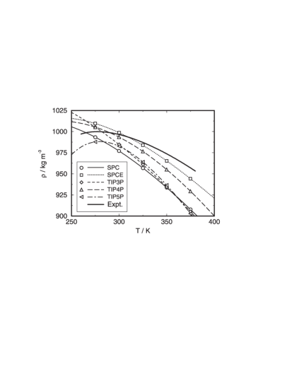
Figure 1: Density of water as a function of temperature for the different water models employed in the present study. The thick solid line represents experimental data according to Wagner and Pruß Wagner and Pruß (2002). The thin lines represent cubic fits to the simulated data (see table 3 for the fitting-parameters).

We would like to point out that our density-fits, although obtained at much higher temperatures, reproduce almost quantitatively the location of the density maxima of SPCE water Baez and Clancy (1994); Harrington et al. (1997); Arbuckle and Clancy (2002) and TIP4P water Tanaka (1996); Mahoney and Jorgensen (2000). The density maxima for SPC and TIP3P are perhaps shifted to even lower temperatures Billeter et al. (1994); Mahoney and Jorgensen (2000) and thus might even lie below a possible glass transition Sciortino et al. (1997).

We would like to emphasise that in line with the temperature dependence of the density, the different models show the same hierarchy with respect to their ability to reproduce waters structural features as shown by the work of Head-Gordon et al. Head-Gordon and Hura (2002); Hura et al. (2000); Sorenson et al. (2000). At ambient conditions the TIP5P model agrees quantitatively with experimental the O-O-structure factor, SPCE and TIP4P agree well, whereas SPC and TIP3P are completely lacking the second peak in the O-O pair correlation function Hura et al. (2000); Sorenson et al. (2000). Hence both structure and density suggest consistently that TIP4P and SPCE might be considered to reflect states of water perhaps at slightly elevated temperature, whereas TIP3P and SPC correspond (structurally) to states of water at much higher temperature. It should be mentioned that all models discussed here show a substantial disagreement with experiment with respect to the OH and HH correlations Head-Gordon and Hura (2002). This might be partially attributed to the fact that the models used here are rigid. But, since as well flexible and polarisable models as well as recent Car-Parinello simulations show the same tendency Head-Gordon and Hura (2002), the reason for this is at present not clear.

Both, solvent structure and density are considered to be of importance for the hydrophobic effects. Since a clear hierarchy of the quality of the water models compared with real water is observed with respect to those properties, the hydrophobic hydration and interaction properties might as well be affected in such a systematic way.

III.2 Hydrophobic Hydration

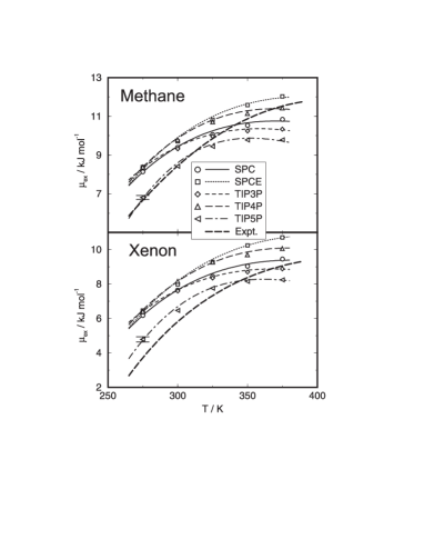
Figure 2: Excess chemical potential of Methane and Xenon in water as a function of temperature. The experimental data (heavy dashed line) are according to Refs. Fernandez-Prini and Crovetto (1998); Wagner and Pruß (2002). The thin lines represent fits to the simulated data employing the MIT-model.

The calculated excess chemical potentials for the noble gases and Methane are shown in Figure 2 and are given in Table 4. The experimental data for Xenon and Methane shown in Figure 2 have been calculated using Henry’s constants according to Fernandez-Prini and Crovetto Fernandez-Prini and Crovetto (1998) employing the water densities for the $0.1\,\mbox{MPa}$ isobar reported by Wagner and Pruß Wagner and Pruß (2002). The thin lines in Figure 2 represent fits of the data to the modified information theory (MIT) model, discussed in section III.3. The corresponding fit parameters are given in Table 5.

The errors for the excess chemical potentials were calculated using the method of Flyvbjerg and Peterson Flyvbjerg and Petersen (1989) and are indicated in Table 4. A further check on the consistency and accuracy of the data has been performed by application of the method of overlapping distribution functions discussed in section A. We would like to point out that the $\mu_{ex}$ data for polarisable Xenon obtained here do only qualitatively agree with the data of Guillot and Guissani Guillot and Guissani (1993). However, test-calculations (results not shown here) performed for selected statepoints given by Guillot and Guissani at higher temperatures Guillot and Guissani (1993) do quantitatively agree, suggesting that the differences at lower temperatures are due to the relatively large statistical error in their calculations and have to be attributed to their rather short simulation runs. Moreover, the obtained value for the excess chemical potential of Methane in TIP4P-water at $300\,\mbox{K}$ of $(9.78\pm 0.1)\,\mbox{kJ}\,\mbox{mol}^{-1}$ agrees well with the value of $(9.79\pm 0.21)\,\mbox{kJ}\,\mbox{mol}^{-1}$ obtained by Shimizu and Chan Shimizu and Chan (2000) for $298\,\mbox{K}$ and $1\,\mbox{atm}$.

		$\mu_{ex}/\mbox{kJ}\,\mbox{mol}^{-1}$							$\Delta\mu_{ex}/\mbox{kJ}\,\mbox{mol}^{-1}$
Model	$T/\mbox{K}$	Ne	Ar	Kr	Xe	$\mbox{Xe}^{\dagger}$	$\mbox{Xe}^{*}$	$\mbox{CH}_{4}$	Xe
SPC	275	10.80	7.64	6.88	6.18		3.39	8.14	-2.59
	300	11.41	8.68	8.12	7.65		4.68	9.39	-3.03
	325	11.76	9.32	8.86	8.44		5.56	10.06	-3.61
	350	11.96	9.77	9.38	9.04		6.22	10.54	-3.95
	375	12.01	10.07	9.75	9.45		6.71	10.84	-4.35
SPCE	275	10.95	7.76	7.06	6.46		3.59	8.38	-2.21
	300	11.73	8.97	8.41	7.99		5.11	9.71	-2.82
	325	12.31	9.94	9.54	9.27		6.08	10.82	-3.24
	350	12.70	10.61	10.37	10.24		7.32	11.58	-3.71
	375	12.90	11.07	10.86	10.71		7.74	12.03	-4.25
SPCE (500 Mol.)	275	10.89	7.66	6.92	6.15	6.16	3.36	8.18
	300	11.69	8.87	8.29	7.71	7.72	5.00	9.56
	325	12.27	9.84	9.41	9.05	8.96	6.22	10.67
	350	12.64	10.52	10.17	9.87	9.88	7.03	11.39
	375	12.84	10.94	10.66	10.41	10.42	7.56	11.83
SPCE (864 Mol.)	275	10.88	7.62	6.80	6.01		3.66	8.09
	300	11.65	8.83	8.20	7.58		4.87	9.45
	325	12.24	9.75	9.24	8.74		6.11	10.54
	350	12.61	10.44	10.05	9.65		6.91	11.26
	375	12.82	10.91	10.63	10.34		7.58	11.78
TIP3P	275	10.94	7.85	7.10	6.40		2.71	8.34	-2.81
	300	11.39	8.69	8.14	7.60		4.09	9.33	-3.30
	325	11.63	9.25	8.79	8.35		4.85	9.97	-3.74
	350	11.72	9.54	9.11	8.69		5.37	10.24	-4.00
	375	11.65	9.66	9.28	8.88		5.77	10.34	-4.32
TIP4P	275	10.88	7.77	7.09	6.40		4.06	8.38	-2.52
	300	11.64	8.99	8.49	8.16		5.82	9.78	-3.13
	325	12.14	9.81	9.44	9.28		6.67	10.71	-3.54
	350	12.39	10.31	9.97	9.70		7.17	11.14	-4.16
	375	12.44	10.59	10.31	10.06		7.53	11.44	-4.43
TIP5P	275	9.76	6.36	5.53	4.79		2.00	6.81	-1.36
	300	10.79	7.84	7.19	6.47		3.34	8.42	-2.46
	325	11.32	8.76	8.23	7.76		4.47	9.44	-3.25
	350	11.45	9.11	8.62	8.16		5.15	9.78	-3.83
	375	11.30	9.16	8.70	8.25		5.33	9.78	-4.02

Table 4: Calculated excess chemical potentials $\mu_{ex}$ for the different solutes along the $0.1\,\mbox{MPa}$ isobar obtained by the particle insertion technique. The $\mbox{Xe}^{*}$ column is obtained by taking the polarisability of $\alpha\!=\!4.11\;\mbox{\AA}^{3}$ into account. The $\mbox{Xe}^{\dagger}$ column contains data accordig to the overlapping distribution method. The data in the most right column represent the change of the chemical potential when bringing a particle from infinity to the distance of the maximum of the Xe-Xe radial distribution function: $\Delta\mu_{ex}=\mu_{ex}(0.42\,\mbox{nm})-\mu_{ex}(\infty)$. The accuracy of the data was estimated to: $\mbox{Ne}:\pm 0.05\,\mbox{kJ}\,\mbox{mol}^{-1}$; $\mbox{Ar}:\pm 0.08\,\mbox{kJ}\,\mbox{mol}^{-1}$; $\mbox{Kr}:\pm 0.1\,\mbox{kJ}\,\mbox{mol}^{-1}$; $\mbox{Xe}:\pm 0.15\,\mbox{kJ}\,\mbox{mol}^{-1}$; $\mbox{Xe}^{*}:\pm 0.25\,\mbox{kJ}\,\mbox{mol}^{-1}$; $\mbox{Xe}^{\dagger}:\pm 0.05\,\mbox{kJ}\,\mbox{mol}^{-1}$; $\mbox{CH}_{4}:\pm 0.1\,\mbox{kJ}\,\mbox{mol}^{-1}$; $\Delta\mu_{ex}(\mbox{Xe}):\pm 0.15\,\mbox{kJ}\,\mbox{mol}^{-1}$.

The SPCE simulations containing larger numbers of molecules (500 and 864) indicate that the excess chemical potentials obtained from 256 water molecules runs are subject to a systematic error of $\mu_{ex}$ due to finite size effects. The observed system-size dependence is presumably due to the restriction of volume fluctuations up to a certain maximum wave-length according to the presence of periodic boundary conditions. As a consequence the values from the 256 molecule simulations are lying systematically too high. As shown in Table 4 this contribution is relatively small for Neon ($\approx 0.1\,\mbox{kJ}\,\mbox{mol}^{-1}$), but increases with particle size and leads to approximately $0.3\,\mbox{kJ}\,\mbox{mol}^{-1}$ and $0.5\,\mbox{kJ}\,\mbox{mol}^{-1}$ too high excess chemical potentials for Methane and Xenon, respectively. However, this difference is found to be only weakly temperature dependent. Therefore the proposition of our paper, a focus on the temperature dependence, is not affected. The shift with respect to the true excess chemical potential can be expected to be in the same range for all models Siepmann et al. (1992) since the compressibilities of the different water models have the same order of magnitude (between $4.6\times 10^{-5}\,\mbox{bar}^{-1}$(SPCE) and $6.0\times 10^{-5}\,\mbox{bar}^{-1}$(TIP3P) at $300\,\mbox{K}$).

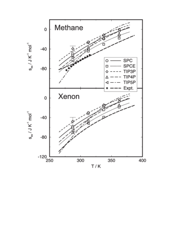
Figure 3: Entropy contribution to the excess chemical potential $s_{ex}$ for Methane and Xenon. The thick dashed lines represent the experimental data according to Fernandez Prini and Crovetto Fernandez-Prini and Crovetto (1998). The closed circles are according to the experimental data of Rettich et al. Rettich et al. (1981). The employed water densities are according to Wagner and Pruß Wagner and Pruß (2002). The lines are according to fits of the $\mu_{ex}$-data to the MIT model, whereas the symbols represent data obtained from finite differences.

Figure 2 reveals that in all cases the simulated excess chemical potentials behave qualitatively like the experimental data in the sense that the excess chemical potential is positive and increases with temperature indicating a negative entropy of solvation. Please note also that around $275\,\mbox{K}$ the simulated excess chemical potentials for all models except for the TIP5P model are lying rather close together, being situated about $2.5\,\mbox{kJ}\,\mbox{mol}^{-1}$ (Methane) and $3.5\,\mbox{kJ}\,\mbox{mol}^{-1}$ (Xenon) above the experimental data. With increasing temperatures, the differences between the values corresponding to the different water models start to increase, already suggesting differently strong solvation entropies. The overall change of $\mu_{ex}$ with temperature is smallest for the TIP3P and SPC model, larger for TIP4P and SPCE and most extreme for the TIP5P model. Please note also that for the TIP3P and TIP5P models the curves for Methane and Xenon suggest the presence of a maximum of $\mu_{ex}$ close to $375\,\mbox{K}$, whereas the experimental maximum is located at much higher temperatures.

In Figure 3 the entropy contribution to the excess chemical potentials are shown for the different models as well as for the experimental data. The thin lines were obtained as numerical derivatives of MIT-model fits whereas the symbols represent finite differences of the $\mu_{ex}$-data given in Table 4. We would like to point out the the experimental data shown here belong to the number density scale and are therefore smaller than the values given in the paper of Rettich et al. Rettich et al. (1981), corresponding to the mole fraction scale. The experimental data shown here were obtained also as a numerical derivative of the experimental excess chemical potentials with respect to the temperature.

A detailed look at the experimental data for Methane according to Fernandez-Prini and Crovetto Fernandez-Prini and Crovetto (1998) reveals decreased slope of $s_{ex}$ in the region below $300\,\mbox{K}$. The reason for this is not quite clear and not present when calculating entropies calculated from the solubility data of Rettich et al. Since this observation Rettich et al. (1981) is also not compatible with the calorimetric measurements of Naghibi et al. Naghibi et al. (1986) it may probably reflect a deficiency of the fit used in Ref. Fernandez-Prini and Crovetto (1998). Above $300\,\mbox{K}$ both experimental datasets, however, do agree well.

The solvation entropy obtained for Methane in TIP4P water at $300\,\mbox{K}$ is found to be $-47\pm 5\,\mbox{J}\,\mbox{K}^{-1}\mbox{mol}^{-1}$, which is slightly larger than the value of $-40.7\,\mbox{J}\,\mbox{K}^{-1}\mbox{mol}^{-1}$ reported by Shimizu and Chan. The entropies are throughout negative, in accordance with the classical interpretation of hydrophobic hydration, suggesting an enhanced ordering of the molecules in the solvation shell. In the region between $275\,\mbox{K}$ and $300\,\mbox{K}$ the experimental data reveal about $15-10\,\mbox{J}\,\mbox{K}^{-1}\mbox{mol}^{-1}$ larger absolute solvation entropies for Xenon compared to Methane. This trend is also observed in the simulations, where we find $7$, $8$, $5$, $7$ and $4\,\mbox{J}\,\mbox{K}^{-1}\mbox{mol}^{-1}$ larger absolute solvation entropies for Xenon for SPC, SPCE, TIP3P, TIP4P and TIP5P-water, respectively. However, the different models show a clear hierarchy with respect to their entropy when comparing with the experimental data for Methane and Xenon. For both cases, Methane and Xenon, TIP3P and SPC exhibit the smallest solvation entropies, whereas TIP4P and SPCE are lying closer to the experimental data. The TIP5P model, however, shows the strongest temperature dependence, exhibiting the about smallest solvation entropy at $275\,\mbox{K}$ of all models and the highest value at $375\,\mbox{K}$. The temperature dependence of the solvation entropies can be quantified in terms of solvation heat capacities. The decrease of the absolute value of the solvation entropies leads to positive solvation heat capacities (calculated for $300\,\mbox{K}$) which are estimated to be $(145\pm 20)$, $(144\pm 20)$, $(145\pm 20)$, $(184\pm 20)$, $(264\pm 20)\,\mbox{J}\,\mbox{K}^{-1}\mbox{mol}^{-1}$ for Methane and $(156\pm 20)$, $(164\pm 20)$, $(160\pm 20)$, $(223\pm 20)$, $(310\pm 20)\,\mbox{J}\,\mbox{K}^{-1}\mbox{mol}^{-1}$ for Xenon in SPC-, SPCE-, TIP3P-, TIP4P- and TIP5P-water, respectively. The experimental data of $c_{P,ex}$ according to the solubility data of Methane of Rettich et al. Rettich et al. (1981) was obtained to be $234\,\mbox{J}\,\mbox{K}^{-1}\mbox{mol}^{-1}$ at $300\,\mbox{K}$, when transforming their data on the number density scale. This value has also been reported by Widom et al. Widom et al. (2003). The value of $c_{P,ex}$ for Xenon according to Fernandez-Prinis data using the same procedure was estimated to be $280\,\mbox{J}\,\mbox{K}^{-1}\mbox{mol}^{-1}$. The general trend, larger absolute solvation entropies and heat-capacities for Xenon compared to Methane, is accomplished by all water models and is also found in experiment. Moreover, the experimental data indicate an increase of the heat capacities at lower temperatures. The fitted curves shown in Figure 3 tend to suggest this as well. However, the error in the entropies obtained from finite differences is perhaps too large to definitely confirm this. The values for $c_{P,ex}$ given above reflect an average considering the whole temperature range.

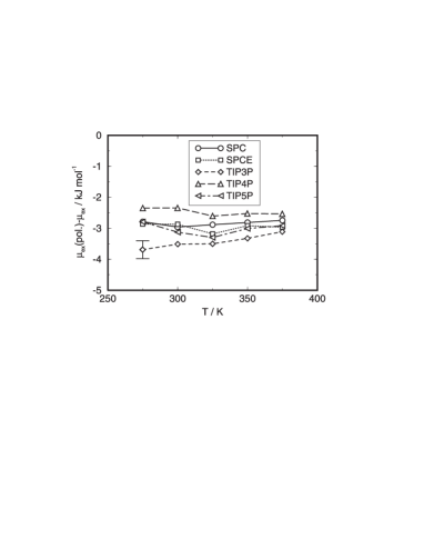
Figure 4: Contribution of the polarisability to the excess chemical potential of Xenon in water.

We would like to point out that the apparent hierarchy of the models with respect to their ability to reproduce waters structure (OO-correlation) and the temperature of maximum density is also observed when comparing the solvation entropies of simple solutes. TIP3P has by far the smallest solvation entropy and the SPC model is only slightly better. SPCE is apparently the best solvent model at higher temperatures (from the point of view of solvation entropies), whereas the TIP5P model is is closer to the experimental data below $300\,\mbox{K}$. Apparently the water models that exhibit a more strongly pronounced structure are also subject to an enhanced ordering of the molecules in the solvation shell, which is reflected by more negative hydration entropies. However, this is perhaps not too surprising, since a water model that provides a better representation of waters structure might as well lead to a more realistic structural description of the hydrophobic hydration shell. The reason for this might be related to the observation that the liquid water structure contains cavities suitable for hydrophobic particles Geiger et al. (1986). This is, of course, also the cause for the Widom particle insertion technique performing so well for hydrophobic particles in water.

The density-curves and corresponding structural features of the individual water models provoked the simplistic interpretation that TIP3P and SPC corresponds structurally to states of water at increased temperature. We would like to point out that the simulated entropies support this point of view. To a first order approximation the simulated entropy-data can be simply corrected by a temperature shift.

Finally, we would like to discuss the effect of having an explicitly polarisable solute particle. As shown in Figure 4, introducing a polarisable Xenon particle leads to a lowering of the chemical potential of about $2.5\,\mbox{kJ}\,\mbox{mol}^{-1}$ to $3.5\,\mbox{kJ}\,\mbox{mol}^{-1}$. Please note that the contribution to the chemical potential due to the polarisability is only weakly temperature dependent. The most extreme cases in this respect are the TIP3P and the TIP4P model. The TIP3P-data show a change of about $0.5\,\mbox{kJ}\,\mbox{mol}^{-1}$ over the entire temperature range, indicating a lowering of the entropy for each temperature on average of about $5\,\mbox{J}\,\mbox{K}^{-1}\mbox{mol}^{-1}$ For the TIP4P model, however, this contribution is about $-2\,\mbox{J}\,\mbox{K}^{-1}\mbox{mol}^{-1}$, leading to a slight increase of the solvation entropy. Both values are lying in the range of the expected error for the entropy values derived from finite difference values of about $\pm 8\,\mbox{J}\,\mbox{K}^{-1}\mbox{mol}^{-1}$.

III.3 A Modified Information Theory Model

Figure 5: Scaling plots of the excess chemical potential of Methane and Xenon in water according to the MIT-model. The MIT-model parameters $c$ and $a$ were obtained as slope and intersection of the data shown here, assuming linearity between $\mu_{ex}\,V_{m}^{2}$ and $V_{m}/T$.

In the previous section we discussed the properties of hydrophobic hydration by relating structural features and solvation entropies employing (to a first order approximation) a temperature shift. In this section we will try to elaborate a more quantitative way to describe the differences between the models.

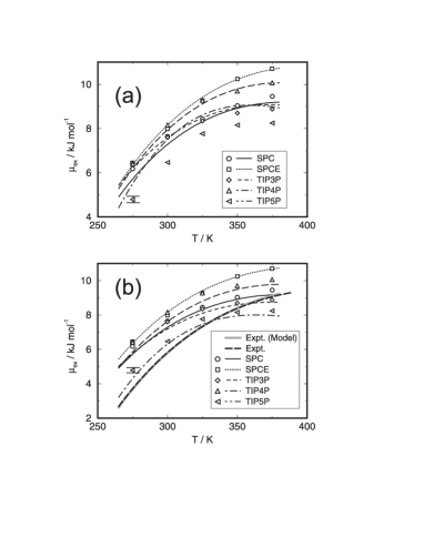
Figure 6: Excess chemical potential of Xenon in water as a function of temperature. (a): The lines represent MIT-Model predictions data using just the parameters obtained for SPCE-water and the different model densities. (b): The lines represent MIT-Model predictions employing the SPCE-parameters, but scaling $a$ by $(\sigma_{\rm Xe-model}/\sigma_{\rm Xe-SPCE})^{6}$. To predict the experimental data a hypothetical “$\sigma_{\rm Xe-model}$” of $3.5275\;\mbox{\AA}$ has been used.

The information theory approach to the hydrophobic hydration according to Hummer et al. Hummer et al. (2000) suggests that the excess chemical potential of a hard sphere particle (i.e. a spherical cavity) can be expressed as

$$\frac{\mu_{ex}}{kT} \approx \frac{v^{2}\rho^{2}}{2\sigma_{n}^{2}}\;,$$ (13)

where $v$ is the volume of the spherical cavity, $\rho$ is the water number density and $\sigma_{n}\!=\!\left<n^{2}\right>-\left<n\right>^{2}$ is the variance of the occupancy number of water molecules in the sphere. For the case of noticeable attractive interactions Hummer et al. Hummer et al. (2000) propose the presence of an additional attractive term plus an offset according to

$$\frac{\mu_{ex}}{kT} \approx A\rho^{2}-C\rho/T+B$$ (14)

where $A\!=\!v^{2}\rho^{2}/(2\sigma_{n}^{2})$ and the parameter $C$ is found to qualitatively account for the effects of attractive solute-solvent interactions Hummer et al. (2000). However, in order to arrive at a quantitative description of the experimental and simulated data, we find it advantageous to express the parameters $A$ and $C$, both inverse proportional to the temperature with

$$A=a^{\prime}/T\;\;\;\mbox{and}\;\;\;C=c^{\prime}/T\;.$$ (15)

The justification for this approach is purely empirical but can be perhaps rationalised as: 1.) An effect of a temperature dependent effective particle diameter, as well as a slight increase in the fluctuation $\sigma_{n}^{2}$ Hummer et al. (2000). At higher temperature, the effective diameter of the solute is likely to decrease due to the form of the repulsive potential. 2.) An effect of a more strongly weakened attractive interaction with increasing temperature. Moreover, when doing this, the offset $B$ can be dropped ($B\!=\!0$), although we must admit that the original model in Eq. 14 using three parameters represents the data slightly better.

Model	MIT-parameters	Ne	Ar	Kr	Xe	$\mbox{Xe}^{*}$	$\mbox{CH}_{4}$	$\mbox{Xe}^{c}$
SPC	$a/10^{-6}\mbox{K}\,\mbox{m}^{6}\mbox{mol}^{-2}$	1.130	1.169	1.213	1.254	1.050	1.272	0.640
	$c/\mbox{K}^{2}\mbox{m}^{3}\mbox{mol}^{-1}$	-10.7	-13.2	-14.3	-15.3	-13.9	-14.4	-7.47
SPCE	$a/10^{-6}\mbox{K}\,\mbox{m}^{6}\mbox{mol}^{-2}$	1.085	1.159	1.218	1.280	1.076	1.271	0.749
	$c/\mbox{K}^{2}\mbox{m}^{3}\mbox{mol}^{-1}$	-10.3	-13.4	-14.7	-16.0	-14.5	-14.7	-9.03
TIP3P	$a/10^{-6}\mbox{K}\,\mbox{m}^{6}\mbox{mol}^{-2}$	1.121	1.138	1.165	1.184	1.002	1.230	0.569
	$c/\mbox{K}^{2}\mbox{m}^{3}\mbox{mol}^{-1}$	-10.8	-12.9	-13.7	-14.4	-13.8	-14.0	-6.54
TIP4P	$a/10^{-6}\mbox{K}\,\mbox{m}^{6}\mbox{mol}^{-2}$	1.096	1.151	1.190	1.240	1.029	1.245	0.654
	$c/\mbox{K}^{2}\mbox{m}^{3}\mbox{mol}^{-1}$	-10.5	-13.1	-14.1	-15.2	-13.3	-14.2	-7.61
TIP5P	$a/10^{-6}\mbox{K}\,\mbox{m}^{6}\mbox{mol}^{-2}$	1.133	1.173	1.200	1.223	0.972	1.256	0.475
	$c/\mbox{K}^{2}\mbox{m}^{3}\mbox{mol}^{-1}$	-11.3	-13.9	-14.8	-15.6	-13.5	-14.9	-5.08
Expt.	$a/10^{-6}\mbox{K}\,\mbox{m}^{6}\mbox{mol}^{-2}$	1.104	1.191	1.212	1.174		1.243
	$c/\mbox{K}^{2}\mbox{m}^{3}\mbox{mol}^{-1}$	-10.9	-14.2	-15.5	-15.7		-15.1

Table 5: Parameters describing the excess chemical potential of the noble gases and Methane applying the modified information theory (MIT) model. The model parameters were obtained by fitting the data of Table 4. The $\mbox{Xe}^{*}$-data corresponds to the polarizable Xe-particle. The $\mbox{Xe}^{c}$-data corresponds a Xenon particle in contact with another Xenon particle. The parameters representing the experimental data were fitted to the data published in Refs. Fernandez-Prini and Crovetto (1998) and Wagner and Pruß (2002).

Since this fitting procedure has been basically inspired by the information theory (IT) approach for hydrophobic hydration and interaction we will refer to it as modified information theory model (MIT) in the course of this paper. Moreover, the parameters $a$ and $c$ are expressed in terms of the molar volume, such that

$$\frac{\mu_{ex}}{R}=\frac{a}{V_{m}^{2}}+\frac{c}{V_{m}\,T}$$ (16)

with $R$ being the ideal gas constant.

In Figure 5 we show scaled plots of the chemical potential of Xenon and Methane according to equation 16. Taking the experimental data, the two parameter MIT model accurately represents the data of the noble gases up to temperatures of $420\mbox{K}-450\mbox{K}$. At higher temperatures the linearity between $\mu_{ex}\,V_{m}^{2}$ and $V_{m}/T$ breaks down, which is not unexpected due to the enhanced increase of the isothermal compressibility $\kappa_{T}$ Hummer et al. (2000). Comparing the obtained MIT-parameters for the noble gases (see Table 5), it is evident that the parameters also behave meaningfully when going from Ne to Xe, in the sense that the $c$-parameters becomes more negative, hence the attractive interaction becomes stronger, whereas the increasing $a$-parameter accounts for the increasing size of the hydrophobic particle.

Nevertheless, the limits of the model become evident also: The slight deviation from linearity for Methane (which is fully absent in the case of Xenon) in Figure 5 becomes significantly stronger in the case of Neon (not shown), indicating that both parameters are subject to a enthalpy-entropy compensation effect and a sufficiently strong attractive (e.g. a large Lennard-Jones $\epsilon$) interaction is required for a good performance of the model. Or in other words: A counterbalancing of the two terms is necessary.

Moreover, it is observed that the $a$ parameter obtained for Xenon is even smaller (or at least very close) to the value obtained for Methane. A stronger attractive interaction apparently leads to a shrinking apparent cavity size which is maybe related to the presence of a more tightly bound hydration shell. This feature is strongly pronounced in the case of the experimental values, here the $a$-parameter for Xenon is even smaller than the value for Krypton. This might be well attributed to the larger polarisability of the Xenon atom compared with Krypton and Methane. As shown in Table 5, taking the polarisability into account significantly reduces the $a$ and $c$.

Figure 5 reveals that the scaled chemical potential data for all models (except for TIP5P) are lying quite close to each other. In addition, the experimental line has almost the same slope, so that the difference between the different models (and experiment) can be described almost completely by just shifting the $a$-parameter. Moreover, the data according to the different models (except for TIP5P) fall almost onto one line. As a consequence it is worthwhile trying to describe the chemical potentials by using the same set of parameters (here we take the data corresponding to the SPCE-model), while just taking the density-curves of the different models into account.

In Figure 6a the Xenon excess chemical potentials for the different water-models, as well as the MIT-model predictions based on the SPCE-parameters are shown. An almost quantitative prediction is achieved, except for the TIP5P model. A possible explanation for the large deviation of TIP5P-data might be the noticeably smaller Lennard-Jones $\sigma$ of the TIP5P-model (see table 1). The information theory suggests that the $a$-parameter should scale with the square of the the particle volume. Hence we try to improve the model prediction by scaling the $a$-parameter with the factor $\left(\sigma_{\rm Xe-model}/\sigma_{\rm Xe-SPCE}\right)^{6}$, shown in Figure 6b, which, indeed, leads to a substantial improvement for the case of TIP5P. In order reproduce the experimental data, a scaling procedure taking the experimental density-curve and and Lennard-Jones parameter of $\sigma_{\rm Xe-Water}\!=\!3.5275\;\mbox{\AA}$ has to be employed.

Apparently the suggested MIT model is able to describe the excess chemical potential of Xennon for the different water models and experiment by just taking the different density isobars into account. In the previous section, however, it was argued that both water structure and the solvation entropies are well related and hence responsible for the performance of the different models. However, this is perhaps not a contradiction when keeping in mind that waters structural and density changes are tightly related and that the transformation towards a more tetrahedrally ordered structure at lower temperatures is the basis for the presence of a density maximum Paschek and Geiger (1999).

We are quite confident that similarities between experimental and simulated data applying the suggested rescaling procedure reveal a signature for hydrophobic hydration in the lower temperature regime and might also be helpful when trying to quantify the interaction between hydrophobic of particles.

III.4 Hydrophobic Interaction

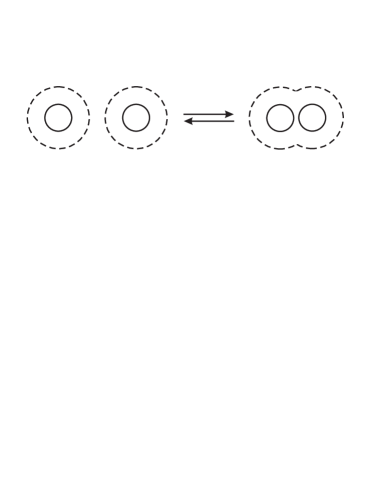
Figure 7: Schematic diagram of the hydrophobic association process according to the classic picture: The contact configuration is stabilised with increasing temperatures by minimising the entropy penalty.

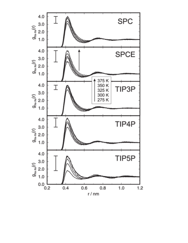
Figure 8: Xe-Xe radial pair distribution functions $g(r)$ for the different water models and temperatures. The arrow indicates the sequence of $g(r)$-curves pointing from low to high temperatures. The bar indicates the change of the height of the first maximum over the whole temperature range.

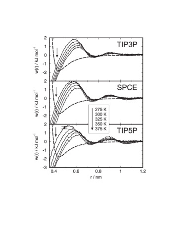
Figure 9: Cavity part of the profile of free energy $w(r)$ obtained for the association of two Xenon particles for three selected models and all temperatures. The heavy dashed lines denote the Xe-Xe Lennard-Jones pair potential.

In order to quantify the hydrophobic interaction we calculate the Xenon-Xenon pair distribution functions for the different models and temperatures. The data are shown Figure 8. All models show an increase of the first peak with rising temperature. This observation is well in accordance with the interpretation that the association of two hydrophobic particles is stabilised by minimising the solvation entropy penalty and has already been reported by a large number of publications Smith et al. (1992); Smith and Haymet (1993); Dang (1994); Lüdemann et al. (1996, 1997); Rick and Berne (1997); Shimizu and Chan (2000); Rick (2000); Shimizu and Chan (2001); Ghosh et al. (2002). The idea is schematically depicted in Figure 7: The enhanced ordering of the solvent molecules in the hydration shell results in a negative solvation entropy. If two particles associate, the corresponding hydration shells overlap, hence leading to a positive net entropy. Consequently contact-configurations should become increasingly stabilised at higher temperatures. In parallel, the increased heat capacity of the water molecules in the hydrophobic hydration shell should lead to a negative heat capacity contribution for the association of two particles, thus weakening the the entropy contribution at elevated temperatures. We would like to emphasise that this model of course lacks completely detailed structural considerations. Our study reveals significant differences for the different water models. The overall maximum variation of the height of the first peak (which is also indicated in Figure 8) is smallest for the TIP3P and SPC models, TIP4P and SPCE show a stronger variation, whereas the TIP5P model reveals an extremely pronounced dropping of the first peak when going to lower temperatures. In all cases the maximum of the first peak is located at a distance of about $4.2\,\mbox{\AA}$, which does not change significantly with varying temperature. Moreover, the pair distributions functions reveal as well the presence of a pronounced second peak corresponding to the solvent separated Xenon-Xenon pair configuration, which is located at $7.2-7.8\,\mbox{\AA}$ and is shifting to smaller distances with decreasing temperatures. In addition, a third maximum, being located at about $10.5\,\mbox{\AA}$, seems to exist at least at the lowest temperatures.

Figure 10: Entropy profile $s(r)$ for the association of two Xenon particles.

In Figure 9 the corresponding profiles of free energy for the association of two Xenon particles are shown. The TIP3P-, SPCE- and TIP5P-water models might be taken here as the representative cases for small, medium and strong temperature variation, respectively. In addition, the relative change of the excess chemical potentials when bringing a Xenon particle from the bulk to the Xenon-Xenon contact distance $\Delta\mu_{ex}\!=\!\mu_{ex}(0.42\,\mbox{nm})-\mu_{ex}(\infty)$ are given in Table 4 for all models and temperatures. We would like to point out that quadratic fits with respect to the temperature describe the changes of data over the entire temperature range reasonably well. From the distribution of pair correlations functions obtained from different parts of the simulation runs, we conclude that the individual curves shown here are accurate within an interval of $\pm 0.15\,\mbox{kJ}\,\mbox{mol}^{-1}$. For completeness Figure 9 contains as well the temperature independent pair potential between two Xenon particles. Figure 9 shows that with decreasing temperature the contact configuration is increasingly destabilised, whereas the solvent separated configuration becomes more and more stable.

Figure 11: Enthalpic and entropic contributions to the cavity part of the profile of free energy $w(r)=h(r)-Ts(r)$. Solid lines: $h(r)$. Dotted lines: $-Ts(r)$.

From the temperature derivative of the $w(r,T)$ data set we obtain the entropy-profiles for the association of two Xenon particles, shown in Figure 10. The entropic $-T\,s(r)$ and enthalpic $h(r)$ contributions to the profile of free energy are given in Figure 11. The temperature variation of the entropy profiles is quantified by the corresponding heat capacity profiles $c_{P}(r)$ given in Figure 14. As already shown by Smith and Haymet Smith et al. (1992); Smith and Haymet (1993) and others, the hydrophobic association process is found to be entropically favoured and enthalpically disfavoured in case of all models. The value of $-5.3\,\mbox{kJ}\,\mbox{mol}^{-1}$ for the entropic contribution to the profile of free energy at $300\,\mbox{K}$ at the contact distance for TIP3P water is reasonably close to the $\approx-3.5\,\mbox{kJ}\,\mbox{mol}^{-1}$ (when taking the data from Figure 5 in Ref. Ghosh et al. (2002)) reported for Methane by Ghosh et al. Ghosh et al. (2002) and the value of $-6.5\,\mbox{kJ}\,\mbox{mol}^{-1}$ is in the same sense consistent with the $-4.14\,\mbox{kJ}\,\mbox{mol}^{-1}$ for Methane in TIP4P water obtained by Shimizu et al.Shimizu and Chan (2000). The observation of slightly larger entropies for the association of Xenon instead of Methane is plausible since the hydration entropies for Xenon are also found to be more negative. We would also like to point out that the hierarchy of the data for the different models according the published data is apparently consistent with our observations. The data of Rick Rick (2000) obtained from simulations employing the polarisable TIP4P-FQ model have been criticised Shimizu and Chan (2000, 2001); Ghosh et al. (2002) because of the unreasonably high heat capacity change for the association of two Methane particles. However, the large entropy contribution to the profile of free energy of about $-12\,\mbox{kJ}\,\mbox{mol}^{-1}$ at the contact distance is rather close to the value of $-11.5\,\mbox{kJ}\,\mbox{mol}^{-1}$ that is observed here for the TIP5P model.

Figure 12: Relative change in heat capcacity $c_{P}(r)$ for the hydrophobic interaction between two dissolved Xenon particles. The data correspond to the temperature derivative of quadratic fits of $w(r,T)$ obtained for $300\,\mbox{K}$. For displaying purposes the data are shifted by an offset of $50\,\mbox{J}\,\mbox{K}^{-1}\,\mbox{mol}^{-1}$.

Figure 10 shows that in all cases there is a tendency for the entropy at very short distances to become smaller with increasing temperature, whereas in the region around $6\,\mbox{\AA}$, at the so called desolvation barrier, the entropy increases with temperature. The general tendency to smaller contact-entropies is in accordance with the decrease of the absolute values of the solvation entropies. However, the distances where the entropy-curves are found to cross each other are quite diverse. Whereas for the TIP-models this region is located around $5.5\,\mbox{\AA}$ it is found in case of the SPC and SPCE models at about $4.5\,\mbox{\AA}$, much closer to the Xenon-Xenon pair distance of about $4.2\,\mbox{\AA}$. As a consequence the pair formation entropies vary much more strongly in case of the TIP models.

From Figure 11 it is evident that in almost all cases the pair configuration is entropically stabilised and enthalpically destabilised. However, TIP5P shows a much stronger enthalpy-entropy compensation effect than all other models, but as well a much stronger variation with temperature. In addition, also the signature of the hydrophobic association vanishes in case of the TIP5P and TIP3P models at $375\,\mbox{K}$ where the entropic and enthalpic contribution to the cavity potential at the the contact distance have almost the same size. This is consistent with finding that in case of the TIP5P and TIP3P models maximum of $\mu_{ex}$ for Xenon is close to $375\,\mbox{K}$ and with the contact entropy $s_{ex}$ being close to zero.

The temperature dependence discussed here can be quantified by the association heat capacities $c_{P}(r)$ shown in Figure 12. Shimizu and Chan Shimizu and Chan (2000, 2001, 2002) report for the association of Methane particles in TIP4P water a change of the heat capacity for the contact state close to zero in qualitative disagreement with the approximate net effect according to the overlapping hydration shells. In addition, they observe a maximum of the heat capacity of about $120\,\mbox{J}\,\mbox{K}^{-1}\,\mbox{mol}^{-1}$ at the location of the desolvation barrier at a distance of $5.5\,\mbox{\AA}$. In a previous study using a polarisable water model Rick Rick (2000) did not observe any peak at the desolvation barrier. Nevertheless, his value of about $-2500\,\,\mbox{J}\,\mbox{K}^{-1}\,\mbox{mol}^{-1}$ for the relative change of heat capacity for the contact state is unreasonably large, being about more than one order of magnitude larger than the solvation heat capacity of Methane found in experiment and the water models used in our study. However, in a more recent study Rick Rick (2003) confirms the presence of a peak at the desolvation barrier of about $40\,\mbox{J}\,\mbox{K}^{-1}\,\mbox{mol}^{-1}$ for the polarizable FQ model. In qualitative agreement with Rick’s recent study Rick (2003) and Shimizu et al. Shimizu and Chan (2001, 2002) and Southall and Dill Southall and Dill (2002) we find that all models show a peak in the heat capacity at the desolvation barrier in the region around $6\,\mbox{\AA}$ of about $20\,\,\mbox{J}\,\mbox{K}^{-1}\,\mbox{mol}^{-1}$ for the TIP3P and SPC model, about $70\,\,\mbox{J}\,\mbox{K}^{-1}\,\mbox{mol}^{-1}$ for the TIP5P and SPCE model and about $50\,\,\mbox{J}\,\mbox{K}^{-1}\,\mbox{mol}^{-1}$ for the TIP4P.

However, for the change in heat capacity for the contact state the different models show a quite diverse behaviour: All TIP models reveal a negative contribution to the heat capacity for the contact state (TIP3P: $-44\,\,\mbox{J}\,\mbox{K}^{-1}\,\mbox{mol}^{-1}$; TIP4P: $-42\,\,\mbox{J}\,\mbox{K}^{-1}\,\mbox{mol}^{-1}$; TIP5P: $-130\,\,\mbox{J}\,\mbox{K}^{-1}\,\mbox{mol}^{-1}$) with the value for the TIP5P model being extremely large. The Berendsen models reveal significantly smaller values with $-23\,\,\mbox{J}\,\mbox{K}^{-1}\,\mbox{mol}^{-1}$ for SPC and $+5\,\,\mbox{J}\,\mbox{K}^{-1}\,\mbox{mol}^{-1}$ for the SPCE model. Hence here we apparently observe for Xenon and the SPCE model what Shimizu and Chan observe for Methane in TIP4P water: A slightly positive heat capacity contribution. The apparent disagreement between the behaviour of Methane and Xenon in TIP4P water, however, might be related to the detailed hydrogen bonding situation (and their flucuations) around the differently sized particles. We would also like to point out that Rick Rick (2003) finds a negative heat capacity contribution for the Methane-Methane contact pair in TIP4P water of about $-140\pm 120\,\mbox{J}\,\mbox{K}^{-1}\,\mbox{mol}^{-1}$.

The apparently smaller heat capacity contributions of the Berendsen-models and the extremely large value found for the TIP5P model, however, strongly suggest that details in the hydrogen bonding situation (i.e. structure of the hydration shell) of the Xenon-Xenon contact state are responsible for the differences. A further detailed comparative analysis concerning the energetics, hydrogen bonding fluctuations and structure of the hydration shell for the different models will help to reveal this differences more clearly and is the topic of a following publication.

III.5 Concerning the Hydrophobic Interaction Between Xenon Particles in Real Water

Figure 13: Scaled plots of the excess chemical potential $\mu_{ex}$ of Xenon in water for the different water models according to the MIT-model. Open symbols: chemical potential obtained for the water bulk. Closed symbols: chemical potential in the vicinity of a Xenon particle (obtained at the distance of the first peak of the Xe-Xe g(r)-function with $r\!=0.42\;\mbox{nm}$). The lines represent MIT fits taking all water models into account. The data corresponding to the lowest temperatures are found on right side of this diagram.

Figure 14: Excess chemical potential of Xenon in the vicinity of another Xenon particle relative to the bulk. The distance corresponds to the maximum of the Xe-Xe $g(r)$-function ($r\!=\!0.42\;\mbox{nm}$). The heavy dashed and dot-dashed lines represents the model prediction for the association of two Xenon particles in real water based on the MIT-parameters for SPCE and TIP5P (see text for details).

In Figure 12 we have applied the rescaling procedure proposed in section III.3 to the chemical potentials of the Xenon particles in contact with another Xenon particle. Again we obtain an apparently linear behaviour for each of the water models, although we must admit that the corresponding slopes are found to vary more strongly than for the case of the bulk liquid. However, it is quite evident that all slopes are considerably smaller than the ones obtained for the bulk. The fit parameters are given in Table 5. An obvious conclusion is of course that the lines corresponding to bulk and shell might have an intersection, defining the temperature where the interaction between the hydrophobic particles turns from attractive into repulsive. The strongest evidence for this scenario comes from the TIP5P data with a value of $\Delta\mu_{ex}(0.42\,\mbox{nm})\!=\!-1.36\,\mbox{kJ}\,\mbox{mol}^{-1}$ at $275\,\mbox{K}$, which is actually weaker than the pure Lennard Jones attraction between the two Xenon particles, indicating an already repulsive water cavity potential. In addition, the destabilisation of the contact-state with decreasing temperature is even enhanced by the increased lowering of the solvent separated minimum of the profile of free energy as shown in Figure 9. The calculated intersection temperature for TIP5P water is found to lie quite high with $257\,\mbox{K}$. For the other water models, however, the prediction of the intersection temperature is much more problematic since the temperatures are apparently shifted to even lower values. Hence the density fits, necessary to determine the intersection temperatures, are much less precise. Therefore the values of about $220\,\mbox{K}$ for SPC and TIP3P and $230\,\mbox{K}$ for SPCE and TIP4P are subject to large uncertainty.

Figure 15: Variation of the strength of the hydrophobic interaction $\Delta\mu(0.42\mbox{nm})\!=\!\mu_{ex}(0.42\mbox{nm})-\mu_{ex}(\infty)$ with the hydration free energy $\mu_{ex}$. The heavy dashed and dot-dashed lines represents the model prediction for the association of two Xenon particles in real water (shown in Figure 14) based on the MIT-parameters for SPCE and TIP5P.

In section III.3 we have shown that the experimental data as well as the TIP5P and SPCE data can be almost quantitatively interrelated by the MIT model assuming an effective Lennard Jones sigma for the experimental water of $\sigma_{\rm Xe-Water}\!=\!3.5375\,\mbox{\AA}$. When applying the same procedure here, however, we should get an impression of how the strength of the hydrophobic interaction of Xenon in real water might behave. We would like to point out that the SPCE and the TIP5P model represent the most extreme cases with respect to their slopes shown in Figure 13. The so calculated strengths of the hydrophobic interaction as a function of temperature are shown in Figure 14 and compared with the corresponding data for the water models. Besides the large uncertainties of this approach, the most striking feature, the strongly changing slope of the $\Delta\mu_{ex}$ curve, is mostly due to the temperature dependence of waters expansivity. Hence this observation does not depend on the exact values of the $a$ and $c$ parameters, but requires just an approximately linear dependence between $\mu_{ex}\,V_{m}^{2}$ and $V_{m}/T$, as it is suggested by all five water models. The corresponding temperatures for the attractive/repulsive conversion are hence found to lie in the interval between $253\,\mbox{K}$ and $267\,\mbox{K}$.

Recently Widom et al. Widom et al. (2003) have deduced from lattice model calculations the presence of an almost linear relation between the hydrophobic interaction $\Delta\mu_{ex}/RT$ and the free energy of hydrophobic hydration $\mu_{ex}/RT$ for the limited temperature interval between $273\,\mbox{K}$ and $333\,\mbox{K}$. Figure 15 shows a such a plot containing the data obtained here for the different water models. Figure 15 indicates that at least for temperatures sufficiently below the maximum of $\mu_{ex}(T)/RT$ their observation is consistent with our data. For the case of the SPCE, TIP4P and TIP5P models an almost linear behaviour in the interval $275\mbox{K}$ and $325\mbox{K}$ is observed. Please note that the model predictions for “real Xenon in water” based MIT model as outlined above behave as well approximately linear for the lower temperatures, suggesting that the MIT predictions for the lower temperatures are as well conceptually consistent with the theory of Widom et al. Widom et al. (2003). We would like to point out that the slope of $0.7$ observed by Widom et al. for Methane is closer to the value of $0.8$ obtained for the TIP5P model than to the $\approx 0.4$ found for SPCE and the other water models.

IV CONCLUSIONS

From a series of Molecular Dynamics simulations on different water models we conclude that the differences between the model waters structure, expansivity behavior and the temperature dependence of the solubility of simple solutes are tightly related. The calculated solvation entropies for all models are found to be systematically smaller than the corresponding experimental values. However, the water models (SPCE, TIP4P, TIP5P) that reproduce waters structure more accurately, provide solvation entropies that are closer to the experimental data.

According to a modification of the Information theory model of Hummer et al. we observe an almost linear dependence between $\mu_{ex}\,V_{m}^{2}$ and $V_{m}/T$ for both experimental and calculated excess chemical potentials. A corresponding rescaling procedure is able to almost eliminate the density dependencies of the different data. Moreover, when taking the size of Xenon particle according to the different Lennard-Jones sigmas for the different models into account, an almost quantitative prediction of the excess chemical potential of Xenon for the different models and the experimental data is feasible.

Concerning the hydrophobic interaction we would like to emphasise the simple fact that all models show a qualitatively similar behaviour: Enhanced aggregation at elevated temperatures. This is in general consistent with the simple picture of the association being driven by entropy effects determined as at net result of overlapping hydrations shells. Nevertheless, from a quantitative point of view noticeable differences between the different models exist, which can only be rationalised considering molecular details of the hydration shell in the Xenon-Xenon contact state. However, in general we can state that the water models that reveal a more realistic hydration entropy and water structure, namely SPCE, TIP4P and TIP5P, reveal as well a more strongly pronounced association behaviour. The TIP5P model reveals an extremely pronounced temperature dependence.

The apparent linear behaviour between $\mu_{ex}\,V_{m}^{2}$ and $V_{m}/T$ is also found for Xenon in the Xenon-Xenon contact state, strongly suggesting the existence of a temperature where the hydrophobic interaction turns from attractive into purely repulsive. For the case of TIP5P water this temperature is found to lie quite high at about $257\,\mbox{K}$. Moreover, the strong temperature dependence of (experimental) waters expansivity strongly indicates that the weakening of the hydrophobic interactions in real water is closer to that obtained for the TIP5P model. Consequently, a model that accounts for waters density effects as closest as possible is as well desirable for a correct description of hydrophobic interactions.

The almost linear relationship between hydrophobic interaction and the strength of hydrophobic hydration proposed by Widom et al. Widom et al. (2003) is at least for temperatures sufficiently below the maximum of $\mu_{ex}(T)/RT$ consistent with our data.

ACKNOWLEGEMENT

I am grateful to Alfons Geiger and Ivan Brovchenko for helpful discussions. Financing by the Deutsche Forschungsgemeinschaft (DFG Forschergruppe 436) is gratefully acknowledged.

Appendix A Appendix: Check on the applicability of the particle insertion technique by the overlapping distribution method in the isobaric-isothermal ensemble

The Widom particle insertion method is known to fail in some cases, such as e.g. the high density Lennard-Jones liquid Frenkel and Smit (2002). In order to confirm that the Widom method can be applied under the conditions of our study we have used additional simulations of one Xenon particle in 500 water molecules to calculate the chemical potential for Xenon using the overlapping distribution method as outlined in Frenkel and Smit (2002); Landau and Binder (2000). The additional simulations were conducted under the same temperatures/pressures and simulation parameters as outlined in section II.1 and extended over 10 ns. Since Xenon is the largest particle in our study, it has the smallest free volume and therefore represents the worst case scenario comparing with other (smaller) noble gases and Methane.

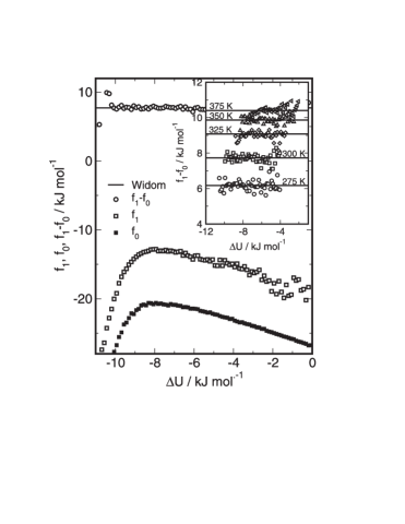
Figure 16: Excess chemical potential $\mu_{ex}$ according to the Widom particle insertion method and the method of overlapping distribution functions. All data were obtained at $p\!=\!0.1\;\mbox{MPa}$ under NPT-conditions. The figure body shows $f_{0}$, $f_{1}$, $f_{1}-f_{0}$ functions and the Widom estimate at $T\!=\!300\;\mbox{K}$. Insert: Well overlapping parts of $f_{1}-f_{0}$ and Widom estimates for all temperatures. All data were obtained from simulations containing 500 SPCE molecules.

Since we are dealing with simulations in the isobaric-isothermal ensemble, the definition of the distribution functions has to be slightly different than that for the canonical ensemble, although this difference is usually ignored Vlot et al. (1999). In analogy to the formulation of the overlapping distribution functions in the canonical ensemble Frenkel and Smit (2002) we define two distribution functions (or histograms) $p_{1}$ and $p_{0}$ of the energy of the $N+1$’th particle $\Delta U\!=\!U(\vec{s}^{N+1};L)-U(\vec{s}^{N};L)$. Here $p_{1}(\Delta U)$ denotes the distribution of energies of the $N+1$’th particle in the $N+1$-particle system in the isobar isothermal ensemble

$$p_{1}(\Delta U) = \frac{1}{Q(N+1,P,T)}\;\frac{\beta P}{\Lambda^{3(N+1)}\,N!}\;\times$$

$$\int dV\int d\vec{s}_{N+1}\int d\vec{s}^{N}\;V^{N+1}\times$$

$$\exp(-\beta PV)\;\exp\left[-\beta U(\vec{s}^{N+1};L)\right]\;\times$$

$$\delta\left(U(\vec{s}^{N+1};L)-U(\vec{s}^{N};L)-\Delta U\right)$$ (17)

where $\beta\!=\!1/kT$ and $\vec{s}_{N}\!=\!L^{-1}\,\vec{r}_{N}$ (with $L\!=\!V^{1/3}$ being the length of a hypothetical cubic box) represent the scaled coordinates of particle $N$. $\vec{s}^{N}$ and $\vec{s}^{N+1}$ represent the set of coordinates of the entire $N$-and $N+1$-particle systems, $P$ is the pressure and $V$ the volume. We have to denote that the partition function contains the factor $N!$ instead of $(N+1)!$ here, since the $N+1$’th particle, the solute particle, is distinguishable from the $N$ solvent particles in case it corresponds to a different particle type. $U(\vec{s}^{N};L)$ and $U(\vec{s}^{N+1};L)$ denote the potential energies of the $N$ and $N+1$ particle systems, respectively. $Q(\ldots)$ is the isobaric isothermal partition function. Eq. A is a straightforward extension of the expression for the canonical ensemble Frenkel and Smit (2002). The function $p_{0}(\Delta U)$ describes the energy-distribution of an additional $N+1$-particle randomly inserted into configurations representing an isobaric-isothermal ensemble of the $N$-particle system. In contrast to the $p_{1}(\Delta U)$ distribution function, the $p_{0}(\Delta U)$ distribution, however, is defined with the instantaneous volume being used as a weighting factor

$$p_{0}(\Delta U) = \frac{1}{Q(N,P,T)}\;\frac{1}{\left<V\right>}\;\frac{\beta P}{\Lambda^{3N}N!}\;\times$$

$$\int dV\int d\vec{s}_{N+1}\int d\vec{s}^{N}\;V^{N}\;\times$$

$$\exp(-\beta PV)\exp\left[-\beta U(\vec{s}^{N};L)\right]\;\times$$

$$V\;\delta\left(U(\vec{s}^{N+1};L)-U(\vec{s}^{N};L)-\Delta U\right)\;,$$ (18)

which has consequently to be normalised by the average volume $\left<V\right>$. Starting with the definition of the $p_{1}(\Delta U)$-distribution function and inserting the definition for $\Delta U$ we come up with the following relation between the two distribution functions

$$p_{1}(\Delta U) = \frac{Q(N,P,T)}{Q(N+1,P,T)}\;\frac{\left<V\right>}{\Lambda^{3}}\;\times$$ (19)

$$= \exp(-\beta\Delta U)\;p_{0}(\Delta U)\;.$$

Using the defition of the ideal and excess part of the chemical potential $\mu$ referring to the ideal gas state with the same average number density in Eq. 2, we obtain a relation between the two distribution functions and the excess chemical potential which is analogous to the expression for the canonical ensemble

$$\ln p_{1}(\Delta U)-\ln p_{0}(\Delta U) = \beta\mu_{ex}-\beta\Delta U\;.$$ (20)

We have to emphasise that the difference, however, is the necessity of volume-weighting in the calculation of the $p_{0}(\Delta U)$-distribution function. As it is usually done Frenkel and Smit (2002), we define functions $f_{0}$ and $f_{1}$ using

$$f_{0}(\Delta U) = \ln p_{0}(\Delta U)-\frac{\beta\Delta U}{2}\;\;\;\hskip 20.00003pt\mbox{and}$$

$$f_{1}(\Delta U) = \ln p_{1}(\Delta U)+\frac{\beta\Delta U}{2}$$

such that

$$\beta\mu_{ex} = f_{1}(\Delta U)-f_{0}(\Delta U)\;.$$ (21)

In most cases the relative volume-fluctuation will be small, and therefore the volume-weighting will cause only a minor modification of to the $p_{0}(\Delta U)$ distribution. However, when considering states close to the critical point, where volume fluctuations might become large, a significant influence cannot be ruled out. Nevertheless, the above formulation should be used in any case, since the volume weighting can be done with practically no additional computational effort.

In Figure 16 the $f_{1}$ and $f_{0}$ distribution functions obtained from the $300\;\mbox{K}$ simulation are shown, as well as difference between both functions and the excess chemical potential obtained from the particle insertion method. The $f_{1}$ and $f_{0}$ distribution functions overlap largely and therefore a rather precise estimation of the excess chemical potential of about $\pm 0.05\;\mbox{kJ}\,\mbox{mol}^{-1}$ is feasible. Figure 16 (see insert) shows a detailed comparison of $f_{1}-f_{0}$-data values according to the Widom method for all temperatures. The values obtained from the Widom particle insertion method agrees quantitatively with the data obtained from to the overlapping distribution method (see also Table 4 for the data) The nice agreement between both methods, can be explained by the form of the $f_{0}$-function. The $f_{0}$ exhibits a maximum, which indicates that the insertion procedure also explores the low-energy edge of the energy distribution with appropriate statistics. As a consequence there is no bias in sampling the energy space and the Widom method provides reliable results. Employing the method of Flyvbjerg and Petersen Flyvbjerg and Petersen (1989) we estimate an error of $\pm 0.1\;\mbox{kJ}\,\mbox{mol}^{-1}$ as an upper bound for the accuracy of the Widom data for Xenon obtained from the 500 molecule system.

References

- Ben-Naim (1980) A. Ben-Naim, Hydrophobic Interactions (Plenum Press, New York, 1980).
- Kauzmann (1959) W. Kauzmann, Adv. Protein Chem. 14, 1 (1959).
- Ben-Naim and Wilf (1979) A. Ben-Naim and J. Wilf, J. Chem. Phys. 70, 771 (1979).
- Privalov and Gill (1988) P. L. Privalov and S. J. Gill, Adv. Protein Chem. 39, 191 (1988).
- Haymet et al. (1996) A. D. J. Haymet, K. A. T. Silverstein, and K. A. Dill, Faraday Discuss. 103, 117 (1996).
- Pierotti (1976) R. A. Pierotti, Chem. Rev. 76, 717 (1976).
- Pratt and Chandler (1977) L. R. Pratt and D. Chandler, J. Chem. Phys. 67, 3683 (1977).
- Smith et al. (1992) D. E. Smith, L. Zhang, and A. D. J. Haymet, J. Am. Chem. Soc. 114, 5875 (1992).
- Smith and Haymet (1993) D. E. Smith and A. D. J. Haymet, J. Chem. Phys. 98, 6445 (1993).
- Geiger et al. (1979) A. Geiger, A. Rahman, and F. H. Stillinger, J. Chem. Phys 70, 263 (1979).
- Zichi and Rossky (1985) D. A. Zichi and P. J. Rossky, J. Chem. Phys. 83, 797 (1985).
- Pearlman (1993) D. A. Pearlman, J. Chem. Phys. 98, 8946 (1993).
- van Belle and Wodak (1993) D. van Belle and S. J. Wodak, J. Am. Chem. Soc 115, 647 (1993).
- Dang (1994) L. X. Dang, J. Chem. Phys. 100, 9032 (1994).
- Forsman and Jönsson (1994) J. Forsman and B. Jönsson, J. Chem. Phys. 101, 5116 (1994).
- Lüdemann et al. (1996) S. Lüdemann, H. Schreiber, R. Abseher, and O. Steinhauser, J. Chem. Phys. 104, 286 (1996).
- Skipper et al. (1996) N. T. Skipper, C. H. Bridgeman, A. D. Buckingham, and R. L. Mancera, Faraday Discuss. 103, 141 (1996).
- Young and Brooks III. (1997) W. S. Young and C. L. Brooks III., J. Chem. Phys. 106, 9265 (1997).
- Hummer et al. (1996) G. Hummer, S. Garde, A. E. Garcia, A. Pohorille, and L. R. Pratt, Proc. Natl. Acad. Sci. USA 93, 8951 (1996).
- Lüdemann et al. (1997) S. Lüdemann, R. Abseher, H. Schreiber, and O. Steinhauser, J. Am. Chem. Soc. 119, 4206 (1997).
- Rick and Berne (1997) S. W. Rick and B. J. Berne, J. Phys. Chem. B 101, 10488 (1997).
- Hummer (2001) G. Hummer, J. Chem. Phys. 114, 7330 (2001).
- Shimizu and Chan (2000) S. Shimizu and H. S. Chan, J. Chem. Phys. 113, 4683 (2000).
- Rick (2000) S. W. Rick, J. Phys. Chem. B 104, 6884 (2000).
- Shimizu and Chan (2001) S. Shimizu and H. S. Chan, J. Am. Chem. Soc 123, 2083 (2001).
- Ghosh et al. (2001) T. Ghosh, A. E. Garcia, and S. Garde, J. Am. Chem. Soc. 123, 10997 (2001).
- Ghosh et al. (2002) T. Ghosh, A. E. Garcia, and S. Garde, J. Chem. Phys 116, 2480 (2002).
- Tanford (1980) C. Tanford, The Hydrophobic Effect: Formation of Micelles and Biological Membranes (John Wiley & Sons, New York, 1980), 2nd ed.
- Huang and Chandler (2000) D. Huang and D. Chandler, Proc. Natl. Acad. Sci. USA 97, 8324 (2000).
- Privalov (1990) P. L. Privalov, Crit. Rev. Biochem. Mol. Biol. 25, 281 (1990).
- Tsai et al. (2002) C. J. Tsai, J. V. Maizel, and R. Nussinov, Crit. Rev. Biochem. Mol. Biol. 37, 55 (2002).
- Kumar et al. (2003) S. Kumar, C. J. Tsai, and R. Nussinov, Biochemistry 42, 4864 (2003).
- Urry (1993) D. W. Urry, Angew. Chem.-Int. Edit. Engl. 32, 819 (1993).
- Darwin et al. (2001) B. L. Darwin, O. V. Alonso, and V. Daggett, J. Mol. Biol. 305, 581 (2001).
- Reiersen et al. (1998) H. Reiersen, A. R. Clarke, and A. R. Rees, J. Mol. Biol. 283, 255 (1998).
- Pratt (2003) L. R. Pratt, Annu. Rev. Phys. Chem. 53, 409 (2003).
- Southall et al. (2002) N. T. Southall, K. A. Dill, and A. D. J.Haymet, J. Phys. Chem. B 106, 521 (2002).
- Smith and Haymet (2003) D. E. Smith and A. D. J. Haymet, in Reviews in Computational Chemistry, edited by K. B. Lipkowitz, R. Larter, and T. R. Cundari (Wiley-VCH, New York, 2003), vol. 19, chap. 2, pp. 44–77.
- Gnanakaran et al. (2003) S. Gnanakaran, H. Nymeyer, J. Portman, K. Y. Sanbonmatsu, and A. E. Garcia, Curr. Opin. Struct. Bio. 13, 168 (2003).
- Sanbonmatsu and Garcia (2002) K. Y. Sanbonmatsu and A. E. Garcia, Proteins: Struct., Funct., Genet. 46, 225 (2002).
- Berendsen et al. (1981) H. J. C. Berendsen, J. P. M. Postma, W. F. van Gunsteren, and J. Hermans, in Intermolecular Forces, edited by B. Pullmann (D. Reidel, Dordrecht, 1981), pp. 331–338.
- Berendsen et al. (1987) H. J. C. Berendsen, J. R. Grigera, and T. P. Straatsma, J. Phys. Chem. 91, 6269 (1987).
- Jorgensen et al. (1983) W. L. Jorgensen, J. Chandrasekhar, J. D. Madura, R. W. Impey, and M. L. Klein, J. Chem. Phys. 79, 926 (1983).
- Mahoney and Jorgensen (2000) M. W. Mahoney and W. L. Jorgensen, J. Chem. Phys. 112, 8910 (2000).
- Pratt and Pohorille (2002) L. R. Pratt and A. Pohorille, Chem. Rev. 102, 2671 (2002).
- Guillot and Guissani (1993) B. Guillot and Y. Guissani, J. Chem. Phys. 99, 8075 (1993).
- Widom et al. (2003) B. Widom, P. Bhimalapuram, and K. Koga, Phys. Chem. Chem. Phys. 5, 3085 (2003).
- Hirschfelder et al. (1954) J. O. Hirschfelder, C. F. Curtiss, and R. B. Bird, Molecular Theory of Gases and Liquids (Wiley, New York, 1954).
- Nosé (1984) S. Nosé, Mol. Phys. 52, 255 (1984).
- Hoover (1985) W. G. Hoover, Phys. Rev. A 31 (1985).
- M. Parrinello (1981) A. R. M. Parrinello, J. Appl. Phys. 52, 7182 (1981).
- Nosé and Klein (1983) S. Nosé and M. L. Klein, Mol. Phys. 50, 1055 (1983).
- Essmann et al. (1995) U. Essmann, L. Perera, M. L. Berkowitz, T. A. Darden, H. Lee, and L. G. Pedersen, J. Chem. Phys. 103, 8577 (1995).
- Miyamoto and Kollman (1992) S. Miyamoto and P. A. Kollman, J. Comp. Chem. 13, 952 (1992).
- Lindahl et al. (2001) E. Lindahl, B. Hess, and D. van der Spoel, J. Mol. Mod. 7, 306 (2001).
- van der Spoel et al. (2001) D. van der Spoel, A. R. van Buuren, E. Apol, P. J. Meulenhoff, D. P. Tieleman, A. L. T. M. Sijbers, B. Hess, K. A. Feenstra, E. Lindahl, R. van Drunen, et al., Gromacs User Manual version 3.1, Nijenborgh 4, 9747 AG Groningen, The Netherlands. Internet: http://www.gromacs.org (2001).
- Flyvbjerg and Petersen (1989) H. Flyvbjerg and H. G. Petersen, J. Chem. Phys. 91, 461 (1989).
- Berendsen et al. (1984) H. J. C. Berendsen, J. P. M. Postma, W. F. van Gunsteren, A. DiNola, and J. R. Haak, J. Chem. Phys. 81, 3684 (1984).
- Siepmann et al. (1992) J. I. Siepmann, I. R. McDonald, and D. Frenkel, J. Phys. Condens. Matter 4, 679 (1992).
- Widom (1963) B. Widom, J. Chem. Phys. 39, 2808 (1963).
- Frenkel and Smit (2002) D. Frenkel and B. Smit, Understanding Molecular Simulation — From Algorithms to Applications (Academic Press, San Diego, 2002), 2nd ed.
- Kennan and Pollack (1990) R. P. Kennan and G. L. Pollack, J. Chem. Phys 93, 2724 (1990).
- Wilhelm et al. (1977) E. Wilhelm, B. R, and R. J. Wilcox, Chem. Rev. 77, 219 (1977).
- Rettich et al. (1981) T. R. Rettich, Y. Handa, R. Battino, and E. Wilhelm, J. Phys. Chem. 85, 3230 (1981).
- Naghibi et al. (1986) H. Naghibi, S. F. Dec, and S. J. Gill, J. Phys. Chem. 90, 4621 (1986).
- Braibanti et al. (1994) A. Braibanti, E. Fisicaro, F. Dallavalle, J. D. Lamb, J. L. Oscarson, and R. Sambasiva Rao, J. Phys. Chem. 98, 626 (1994).
- Ben-Naim (1978) A. Ben-Naim, J. Phys. Chem. 82, 792 (1978).
- Deitrick et al. (1989) G. L. Deitrick, L. E. Scriven, and H. T. Davis, J. Chem. Phys. 90, 2370 (1989).
- Deitrick et al. (1992) G. L. Deitrick, L. E. Scriven, and H. Davis, Molecular Simulation 8, 239 (1992).
- Lisal et al. (2002) M. Lisal, J. Kolafa, and I. Nezbeda, J. Chem. Phys. 117, 8892 (2002).
- Wagner and Pruß (2002) W. Wagner and A. Pruß, J. Phys. Chem. Ref. Data 31, 387 (2002).
- Baez and Clancy (1994) L. A. Baez and P. Clancy, J. Phys. Chem. 101, 9837 (1994).
- Harrington et al. (1997) S. Harrington, P. H. Poole, F. Sciortino, and H. E. Stanley, J. Chem. Phys. 107, 7443 (1997).
- Arbuckle and Clancy (2002) B. W. Arbuckle and P. Clancy, J. Chem. Phys. 116, 5090 (2002).
- Tanaka (1996) H. Tanaka, J. Chem. Phys. 105, 5099 (1996).
- Billeter et al. (1994) S. R. Billeter, P. M. King, and W. F. van Gunsteren, J. Chem. Phys. 100, 6692 (1994).
- Sciortino et al. (1997) F. Sciortino, L. Fabbian, S. H. Chen, and P. Tartaglia, Phys. Rev. E 56, 5397 (1997).
- Head-Gordon and Hura (2002) T. Head-Gordon and G. Hura, Chem. Rev. 102, 2651 (2002).
- Hura et al. (2000) G. Hura, J. M. Sorenson, R. M. Glaeser, and T. Head-Gordon, J. Chem. Phys. 113, 9140 (2000).
- Sorenson et al. (2000) J. M. Sorenson, G. Hura, R. M. Glaeser, and T. Head-Gordon, J. Chem. Phys. 113, 9149 (2000).
- Fernandez-Prini and Crovetto (1998) R. Fernandez-Prini and R. Crovetto, J. Phys. Chem. Ref. Data 18, 1231 (1998).
- Geiger et al. (1986) A. Geiger, P. Mausbach, and J. Schnitker, in Water and Aqueous Solutions, edited by G. W. Neilson and J. E. Enderby (Adam Hilger, Bristol, 1986), pp. 15–30.
- Hummer et al. (2000) G. Hummer, D. Garde, A. E. Garcia, and L. R. Pratt, Chem. Phys. 258, 349 (2000).
- Paschek and Geiger (1999) D. Paschek and A. Geiger, J. Phys. Chem. B 103, 4139 (1999).
- Shimizu and Chan (2002) S. Shimizu and H. Chan, Proteins: Struct., Funct., Genet. pp. 560–566 (2002).
- Rick (2003) S. W. Rick, J. Chem. Phys. B 107, 9853 (2003).
- Southall and Dill (2002) N. T. Southall and K. A. Dill, Biophys. Chem. 101–102, 295 (2002).
- Landau and Binder (2000) D. P. Landau and K. Binder, A Guide to Monte Carlo Simulations in Statistical Physics (Cambrige University Press, Cambrige, 2000).
- Vlot et al. (1999) M. J. Vlot, J. Huinink, and P. van der Eeerden, J. Chem. Phys. 110, 55 (1999).