Atom-molecule coherence in Bose gases
Abstract
In an atomic gas near a Feshbach resonance, the energy of two colliding atoms is close to the energy of a bound state, i.e., a molecular state, in a closed channel that is coupled to the incoming open channel. Due to the different spin arrangements of the atoms in the open channel and the atoms in the molecular state, the energy difference between the bound state and the two-atom continuum threshold is experimentally accessible by means of the Zeeman interaction of the atomic spins with a magnetic field. As a result, it is in principle possible to vary the scattering length to any value by tuning the magnetic field. This level of experimental control has opened the road for many beautiful experiments, which recently led to the demonstration of coherence between atoms and molecules. This is achieved by observing coherent oscillations between atoms and molecules, analogous to coherent Rabi oscillations that occur in ordinary two-level systems. We review the many-body theory that describes coherence between atoms and molecules in terms of an effective quantum field theory for Feshbach-resonant interactions. The most important feature of this effective quantum field theory is that it incorporates the two-atom physics of the Feshbach resonance exactly, which turns out to be necessary to fully explain experiments with Bose-Einstein condensed atomic gases.
keywords:
Bose-Einstein condensation , Feshbach resonance , Coherent matter waves , Many-body theoryPACS:
03.75.Kk, 67.40.-w, 32.80.Pjurl]http://www.phys.uu.nl/~duine and
1 Introduction
Following the first experimental realization of Bose-Einstein condensation [1], a great deal of experimental and theoretical progress has been made in the field of ultracold atomic gases [2, 3, 4, 5]. One particular reason for this progress is the unprecedented experimental control over the atomic gases of interest. This experimental control over the ultracold magnetically-trapped alkali gases, has recently culminated in the demonstration of experimentally adjustable interactions between the atoms [6]. This is achieved by means of a so-called Feshbach resonance [7].
Feshbach resonances were introduced in nuclear physics to describe the narrow resonances observed in the total cross section for a neutron scattering of a nucleus [8]. These very narrow resonances are the result of the formation of a long-lived compound nucleus during the scattering process, with a binding energy close to that of the incoming neutron. The defining feature of a Feshbach resonance is that the bound state responsible for the resonance exists in another part of the quantum-mechanical Hilbert space than the part associated with the incoming particles. In the simplest case, these two parts of the Hilbert space are referred to as the closed and open channel, respectively.
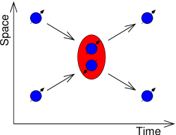
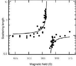
Following these ideas from nuclear physics, Stwalley [9] and Tiesinga et al. [10] considered Feshbach resonances in ultracold doubly spin-polarized alkali gases. Due to the low temperatures of these gases, their effective interatomic interactions are to a large extent completely determined by the -wave scattering length. Analogous to the formation of a compound nucleus in neutron scattering, two atoms can form a long-lived bound state, i.e., a diatomic molecule, during an -wave collision. This process is illustrated in Fig. 1. The two incoming atoms in the open channel have a different hyperfine state than the bound state in the closed channel and the coupling between the open and closed channel is provided by the exchange interaction. As a result of this difference in the hyperfine state, the two channels have a different Zeeman shift in a magnetic field. Therefore, the energy difference between the closed-channel bound state and the two-atom continuum threshold, the so-called detuning, is experimentally adjustable by tuning the magnetic field. This implies that the -wave scattering length, and hence the magnitude and sign of the interatomic interactions, is also adjustable to any desirable value. In Fig. 2 the scattering length, as measured by Inouye et al. [6], is shown as a function of the magnetic field. The position of the resonance in the magnetic field is at (G)auss in this case. Following this first experimental observation of Feshbach resonances in 23Na [6], they have now been observed in various bosonic atomic species [11, 12, 13, 14, 15], as well as a number of fermionic isotopes [16, 17, 18, 19].
With this experimental degree of freedom it is possible to study very interesting new regimes in the many-body physics of ultracold atomic gases. The first experimental application was the detailed study of the collapse of a condensate with attractive interactions, corresponding to negative scattering lengths. In general a collapse occurs when the attractive interactions overcome the stabilizing kinetic energy of the condensate atoms in the trap. Since the typical interaction energy is proportional to the density, there is a certain maximum number of atoms above which the condensate is unstable [20, 21, 22, 23, 24]. In the first observations of the condensate collapse by Bradley et al. [25], a condensate of doubly spin-polarized 7Li atoms was used. In these experiments the atoms have a fixed negative scattering length which for the experimental trap parameters lead to a maximum number of condensate atoms that was so small that nondestructive imaging of the condensate was impossible. Moreover, thermal fluctuations due to a large thermal component made the initiation of the collapse a stochastic process [26], thus preventing also a series of destructive measurements of a single collapse event [27]. A statistical analysis has nevertheless resulted in important information about the collapse process [28]. Very recently, it was even possible to overcome these complications [29].
In addition to the experiment with 7Li, experiments with 85Rb have been carried out [30]. In particular, Roberts et al. [31] also studied the stability criterion for the condensate, and Donley et al. [32] studied the dynamics of a single collapse event in great detail. Both of these experiments make use of a Feshbach resonance to achieve a well-defined initial condition for each destructive measurement. It turns out that during a collapse a significant fraction of atoms is expelled from the condensate. Moreover, one observes a burst of hot atoms with an energy of about nK. Several mean-field analyses of the collapse, which model the atom loss phenomenologically by a three-body recombination rate constant [33, 34, 35, 36, 37, 38, 39], as well as an approach that considers elastic condensate collisions [40, 41], and an approach that takes into account the formation of molecules [42], have offered a great deal of theoretical insight. Nevertheless, the physical mechanism responsible for the explosion of atoms out of the condensate and the formation of the noncondensed component is to a great extent still not understood at present.
A second experimental application of a Feshbach resonance in a Bose-Einstein condensed gas is the observation of a bright soliton train by Strecker et al. [15]. In this experiment, one starts with a large one-dimensional Bose-Einstein condensate of 7Li atoms with positive scattering length near a Feshbach resonance. The scattering length is then abruptly changed to a negative value. Due to its one-dimensional nature the condensate does not collapse, but instead forms a train of on average four bright solitary waves that repel each other. The formation of these bright solitons is the result of phase fluctuations [43], which are in this case important due to the low dimensionality [44, 45, 46, 47, 48, 49]. The repulsion between the bright solitons is a result of their relative phase difference of about . In a similar experiment Khaykovich et al. [50] have observed the formation of a single bright soliton.
A third experimental application are the experiments with trapped gases of fermionic atoms, where the objective is to cool the gas down to temperatures where the so-called BCS transition, i.e., the Bose-Einstein condensation of Cooper pairs, may be observed. The BCS transition temperature increases if the scattering length is more negative [51], and hence a Feshbach resonance can possibly be used to make the transition experimentally less difficult to achieve. This possibility has inspired the study of many-body effects in fermionic gases near a Feshbach resonance [52, 53, 54, 55, 56, 57, 58], as well as fluctuation effects on the critical temperature [59, 60]. One of the most interesting features of a fermionic gas near a Feshbach resonance is the crossover between a condensate of Cooper pairs and a condensate of molecules, the so-called BCS-BEC crossover that was recently studied by Ohashi and Griffin [55, 56, 57] on the basis of the Nozières-Schmitt-Rink formalism [61]. As a first step towards this crossover, Regal et al. [62] were recently able to convert a fraction of the atoms in a gas of fermionic atoms in the normal state into diatomic molecules, by sweeping the magnetic field across a Feshbach resonance. Following this observation, Strecker et al. observed the formation of long-lived 6Li2 molecules [63], and Xu et al. observed 23Na molecules [64]. Very recently, even the formation of Bose-Einstein condensates of molecules has been observed by Jochim et al. [65], Greiner et al. [66], and by Zwierlein et al. [67]. As another application of Feshbach resonances in fermionic gases we mention here also the theoretical proposal by Falco et al. to observe a new manifestation of the Kondo effect in these systems [68].
The experimental application on which we focus in this paper is the observation of coherent atom-molecule oscillations [69]. These experiments are inspired by the theoretical proposal of Drummond et al. [70] and Timmermans et al. [71] to describe the Feshbach-resonant part of the interactions between the atoms in a Bose-Einstein condensate by a coupling of the atomic condensate to a molecular condensate. For this physical picture to be valid, there has to be a well-defined phase between the wave function that describes the atoms in the atomic condensate, and its molecular counterpart. An equivalent statement is that there is coherence between the atoms and the molecules. Since the energy difference between the atoms and the molecular state is experimentally tunable by adjusting the magnetic field, it is, with this physical picture in mind, natural to perform a Rabi experiment by means of one pulse in the magnetic field towards resonance, and to perform a Ramsey experiment consisting of two short pulses in the magnetic field. If the physical picture is correct we expect to observe oscillations in the remaining number of condensate atoms in both cases.
In the first experiment along these lines, Claussen et al. [72] started from a Bose-Einstein condensate of 85Rb atoms without a visible thermal cloud and tuned the magnetic field such that the atoms were effectively noninteracting. With this atomic species this is possible, because the off-resonant background scattering length is negative, which can be compensated for by making the resonant part of the scattering length positive. Next, one applied a trapezoidal pulse in the magnetic field, directed towards resonance. As a function of the duration of the pulse one observed that the number of atoms first decreases but after some time increases again. This increase can not be explained by a “conventional” loss process, such as dipolar relaxation or three-body recombination, since the magnitude of the loss is in these cases given by a rate constant times the square and the cube of the density, respectively. As a result, the loss always increases with longer times. A theoretical description of this experiment is complicated by the fact that the experiment is at long times close to the resonance where little is known about the magnetic-field dependence of these rate constants. Although the magnetic-field dependence has been calculated for a shape resonance [73, 74, 75, 76], it is not immediately obvious that the results carry over to the multichannel situation of a Feshbach resonance. Moreover, precise experimental data is unavailable [77]. Therefore a satisfying quantitative description is still lacking, although two attempts have been made [41, 78].
After these experiments, the same group performed an experiment consisting of two short pulses in the magnetic field towards resonance, separated by a longer evolution time [69]. As a function of this evolution time an oscillation in the number of condensate atoms was observed. Over the investigated range of magnetic field during the evolution time, the frequency of this oscillation agreed exactly with the molecular binding energy found from a two-atom coupled-channels calculation [79], indicating coherence between atoms and molecules. Very recently, Claussen et al. have performed a similar series of measurements over a larger range of magnetic fields [80]. It was found that close to resonance the frequency of the oscillation deviates from the vacuum molecular binding energy as a result of many-body effects [81, 82].
As already mentioned, the first theories for Feshbach-resonant interactions introduce the physical picture of an interacting atomic Bose-Einstein condensate coupled to a noninteracting molecular condensate [70, 71, 83]. The first description of the Ramsey experiments by Donley et al. [69] was achieved within the Hartree-Fock-Bogoliubov mean-field theory [79, 78, 84].
It turns out that, for a complete understanding of the experiments, it is necessary to exactly incorporate the two-atom physics into the theory. Although the above-mentioned theories have provided a first understanding of the physics of a Bose gas near a Feshbach resonance, these many-body theories do not contain the two-atom collision properties exactly. To incorporate the two-atom physics exactly, it is from a diagrammatic point of view required to sum all the ladder Feynman diagrams of the microscopic theory. By means of this procedure, we have recently derived an effective quantum field theory describing the many-body properties of an atomic gas near a Feshbach resonance [85]. It is the aim of this paper to review and extend this effective atom-molecule theory and its applications [85, 81, 82]. Moreover, along the way we discuss some of the differences and similarities between our theory and a number of other theories for Feshbach-resonant interactions in atomic Bose gases [70, 71, 83, 79, 78, 84, 86, 87, 88, 89, 90].
With this objective in mind, this paper is organized as follows. In Section 2 we review two-atom scattering theory. In particular, we emphasize the relation between the scattering amplitude of a potential and its bound states. Both the single-channel case, as well as the multichannel case that can give rise to Feshbach resonances, are discussed. This introductory section introduces many important concepts in a simple setting, and hence clarifies much of the physics that is discussed in later sections. In Section 3 we present in detail the derivation of an effective quantum field theory applicable for studying many-body properties of the system, starting from the microscopic atomic hamiltonian for a Feshbach resonance. This effective field theory consists of an atomic quantum field that is coupled to a molecular quantum field responsible for the Feshbach resonance. It is used in Section 4 to study the normal state of the gas. In particular, we show here that the two-atom scattering properties as well as the molecular binding energy are correctly incorporated into the theory. Moreover, we also discuss many-body effects on the molecular binding energy. Section 5 is devoted to the discussion of the Bose-Einstein condensed phase of the gas. We derive the mean-field theory resulting from our quantum field theory. We also discuss the differences and similarities between this mean-field theory and in particular the mean-field theories that were recently proposed by Kokkelmans and Holland [79], Mackie et al. [78], and Köhler et al. [84]. In Section 6 our mean-field theory is applied to the two-pulse experiments [69, 80]. It is the perfect agreement between theory and experiment obtained in this section that ultimately justifies the ab initio approach to Bose gases near a Feshbach resonance reviewed in this paper. We end in Section 7 with our conclusions.
2 Scattering and bound states
In this section we give a review of quantum-mechanical scattering theory. We focus on the relation between the scattering amplitude of a potential and its bound states [91, 92]. In the first part we consider single-channel scattering and focus on the example of the square well. In the second part we consider the situation of two coupled channels, which can give rise to a Feshbach resonance.
2.1 Single-channel scattering: an example
We consider the situation of two atoms of mass that interact via the potential that vanishes for large distances between the atoms. The motion of the atoms separates into the trivial center-of-mass motion and the relative motion, described by the wave function where , and and are the coordinates of the two atoms, respectively. This wave function is determined by the time-independent Schrödinger equation
| (1) |
with the energy of the atoms in the center-of-mass system. Solutions of the Schrödinger equation with negative energy correspond to bound states of the potential, i.e., to molecular states. To describe atom-atom scattering we have to look for solutions with positive energy , with the kinetic energy of a single atom with momentum . Since any realistic interatomic interaction potential vanishes rapidly as the distance between the atoms becomes large, we know that the solution for of Eq. (1) is given by a superposition of incoming and outgoing plane waves. More precisely, the scattering wave function is given by an incoming plane wave and an outgoing spherical wave and reads
| (2) |
where the function is known as the scattering amplitude. The interatomic interaction potential depends only on the distance between the atoms and hence the scattering amplitude depends only on the angle between and , and the magnitude . Because of energy conservation we have that . The situation is shown schematically in Fig. 3.

Following the partial-wave method we expand the scattering amplitude in Legendre polynomials according to
| (3) |
The wave function is expanded in a similar manner as
| (4) |
with the radial wave function and determined by the radial Schrödinger equation
| (5) |
By expanding also the incident plane wave in partial waves according to
| (6) |
we can show that to obey the boundary condition in Eq. (2), the partial-wave amplitudes have to be of the form
| (7) |
where is the so-called phase shift of the -th partial wave.
For the ultracold alkali atoms, we are allowed to consider only -wave scattering, since the colliding atoms have too low energies to penetrate the centrifugal barrier in the effective hamiltonian in Eq. (5). Moreover, as we see later on, the low-energy effective interactions between the atoms are fully determined by the -wave scattering length, defined by
| (8) |
From Eq. (7) we find that the -wave scattering amplitude is given by
| (9) |
As explained above, we take only the -wave contribution into account, which gives for the scattering amplitude at zero-momentum
| (10) |
To illustrate the physical meaning of the -wave scattering length, we now calculate it explicitly for the simple case that the interaction potential is a square well. We thus take the interaction potential of the form
| (13) |
with . With this potential, the general solution of Eq. (5) for is given by
| (16) |
with . Since the wave function has to obey the Schrödinger equation at the origin we have to demand that the function vanishes at this point. This leads to the boundary condition . By comparing the explicit form of the wave function with the -wave component of the general scattering wave function for , we find that
| (17) |
Hence, we determine the phase shift by demanding that the wave functions for and join smoothly. This leads to the equations
| (18) |
where we have chosen the normalization such that . Multiplication of the above equations with and dividing the result leads to
| (19) |
from which it follows that
| (20) |
Note that for a repulsive hard-core potential we have that and therefore, with the use of the definition in Eq. (8), that the scattering length . This immediately gives a physical picture for a positive -wave scattering length: at low energy and momenta the details of the potential are unimportant and we are allowed to model the potential with an effective hard-core potential of radius . For a fully repulsive potential the scattering length is always positive. For a potential with attractive parts the scattering length can be both negative and positive, corresponding to attractive and repulsive effective interactions, respectively.

This is seen by explicitly calculating the scattering length for our example in the case that . As its definition in Eq. (8) shows, the scattering length is determined by the linear dependence of the phase shift on the magnitude of the relative momentum of the scattering atoms for small momentum. Generally, the phase shift can be expanded according to [91, 92, 93]
| (21) |
from which the scattering length is determined by
| (22) |
with a dimensionless constant. The parameter is the so-called effective range and is, in our example of the square-well potential, given by
| (23) |
In Fig. 4 the scattering length is shown as a function of by the solid line. Clearly, the scattering length can be both negative and positive, and becomes equal to zero at values of such that . In the same figure, the effective range is shown by the dashed line. Note that the effective range diverges if the scattering length becomes equal to zero. This is because the expansion in Eq. (21) is ill-defined for . At values of with a positive integer the scattering length diverges and changes sign. This behaviour is called a potential or shape resonance and in fact occurs each time the potential is just deep enough to support a new bound state. Therefore, for large and positive scattering length the square well has a bound state with an energy just below the continuum threshold. It turns out that there is an important relationship between the energy of this bound state and the scattering length.
To find this relation we have to determine the bound-state energy by solving the Schödinger equation for negative energy . This leads to solutions
| (26) |
with and . Demanding again that these solutions join smoothly at , we find the equation for the bound-state energy
| (27) |
We can show that for values of such that this equation has solutions for [92].
For small binding energy we have from the equation for the bound-state energy that
| (28) |
where we made use of the fact that has to be close to the resonant values in this case. This leads to the desired relation between the energy of the molecular state and the scattering length given by
| (29) |
This result does not depend on the specific details of the potential and it turns out to be quite general. Any potential with a large positive scattering length has a bound state just below the continuum threshold with energy given by Eq. (29). Moreover, the relation will turn out to hold also in the multichannel case of a Feshbach resonance as we will see in Section 2.3. Before discussing this situation, we first turn to some concepts of scattering theory which are of importance for the remainder of this paper.
2.2 Single-channel scattering: formal treatment
Let us give a more formal treatment of the scattering theory described above. In a basis-independent formulation the Schrödinger equation we have solved reads
| (30) |
with the relative kinetic energy operator for the atoms. To describe scattering, we have to look for solutions which asymptotically represent an incoming plane wave, and an outgoing spherical wave. In the absence of the potential there is no scattering, and hence we demand that the solution of Eq. (30) reduces to a plane wave in the limit of vanishing potential. The formal solution that obeys this condition is given by
| (31) |
where represents the incoming plane wave and we recall that is the kinetic energy of the atoms. This energy is made slightly complex by the usual limiting procedure . Moreover, we have for the scattering amplitude that
| (32) |
To determine the scattering amplitude directly, we introduce the two-body T(ransition) matrix by means of
| (33) |
Multiplying the formal solution in Eq. (31) by we have that
| (34) |
Since this equation holds for an arbitrary plane wave and because these plane waves form a complete set of states we have the following operator equation for the two-body T-matrix
| (35) |
This equation is called the Lippmann-Schwinger equation and from its solution we are able to determine the scattering properties of the potential . To see this we first note that from the definition of the T-matrix in Eq. (33), together with Eq. (32), it follows immediately that
| (36) |
Therefore, we indeed see that the two-body T-matrix completely determines the scattering amplitude. The Lippmann-Schwinger equation for the two-body T-matrix can be solved in perturbation theory in the potential. This results in the so-called Born series given by
| (37) |
where
| (38) |
is the noninteracting propagator of the atoms. By using, instead of the true interatomic interaction potential, a pseudopotential of the form
| (39) |
the first term in the Born series immediately yields the correct result for the scattering amplitude at low energies and momenta, given in Eq. (10). Such a pseudopotential should therefore not be used to calculate higher-order terms in the Born series, but should be used only in first-order perturbation theory.
The poles of the T-matrix in the complex-energy plane correspond to bound states of the potential. To see this we note that the formal solution of the Lippmann-Schwinger equation is given by
| (40) |
After insertion of the complete set of eigenstates of we have
| (41) |
where the summation over is discrete for the bound-state energies , and represents an integration for positive energies that correspond to scattering solutions of the Schrödinger equation, so explicitly we have that
| (42) |
From this equation we clearly see that the two-body T-matrix has poles in the complex-energy plane, corresponding to the bound states of the potential. In addition, the T-matrix contains a branch cut on the positive real axis due to the continuum of scattering states.
As an example, we note that for -wave scattering the T-matrix is independent of the angle between and . From the relation between the T-matrix and the scattering amplitude, and the expression for the latter in terms of the phase shift, we have for low positive energies
| (43) | |||||
where we made use of the expansion in Eq. (21). From this result we deduce by analytic continuation that
| (44) |
Clearly, for large and positive scattering length the T-matrix has a pole at negative energy , in complete agreement with our previous discussions.
Summarizing, we have found that the scattering length of an attractive potential well can have any value and depends strongly on the energy of the weakliest bound state in the potential. In principle therefore, if we have experimental access to the energy difference of this bound state and the continuum threshold we are able to experimentally alter the scattering length and thereby the effective interactions of the atoms. In the single-channel case this is basically impossible to achieve. In a multichannel system, however, the energy difference is experimentally accessible, which makes the low-energy effective interactions between the atoms tunable. In the next section we discuss this situation.
2.3 Example of a Feshbach resonance
We consider now the situation of atom-atom scattering where the atoms have two internal states [94]. These states correspond, roughly speaking, to the eigenstates of the spin operator of the valence electron of the alkali atoms. The effective interaction potential between the atoms depends on the state of the valence electrons of the colliding atoms. If these form a singlet the electrons are in principle allowed to be on top of each other. For a triplet this is forbidden. Hence, the singlet potential is generally much deeper than the triplet potential.
Of course, in reality the atom also has a nucleus with spin which interacts with the spin of the electron via the hyperfine interaction
| (45) |
with the hyperfine constant. The hyperfine interaction couples the singlet and triplet states. Moreover, in the presence of a magnetic field the different internal states of the atoms have a different Zeeman shift. In an experiment with magnetically-trapped gases, the energy difference between these states is therefore experimentally accessible. Putting these results together, we can write down the Schödinger equation that models the above physics
| (50) |
Here, and are the interaction potentials of atoms with internal state and , respectively, and is their difference in Zeeman energy due to the interaction with the magnetic field , with the difference in magnetic moment. In agreement with the above remarks, is referred to as the triplet channel, whereas is referred to as the singlet channel. The potentials and are the triplet and singlet interaction potentials, respectively.
As a specific example, we use for both interaction potentials again square well potentials,
| (51) |
where . For convenience we have taken the range the same for both potentials. Furthermore, we assume that the potentials are such that and that is just deep enough such that it contains exactly one bound state. Finally, we assume that . The potentials are shown in Fig. 5.
To discuss the scattering properties of the atoms, we have to diagonalize the hamiltonian for , in order to determine the incoming channels, which are superpositions of the triplet and singlet states and . Since the kinetic energy operator is diagonal in the internal space of the atoms, we have to find the eigenvalues of the hamiltonian
| (54) |
These are given by
| (55) |
The hamiltonian is diagonalized by the matrix
| (58) |
according to
| (61) |
which determines . We define now the hyperfine states and according to
| (66) |
which asymptotically represent the scattering channels. In this basis the Schrödinger equation for all reads
| (69) | |||
| (72) |
where the energy is measured with respect to and we have defined the potentials according to
| (73) |
Since all these potentials vanish for we can study scattering of atoms in the states and . Because the hyperfine interaction is small we have that and . Moreover, for the experiments with magnetically-trapped gases we always have that where is Boltzmann’s constant and is the temperature. This means that in a realistic atomic gas, in which the states and are available, there are in equilibrium almost no atoms that scatter via the latter state. Because of this, the effects of the interactions of the atoms will be determined by the scattering amplitude in the state . If two atoms scatter in this channel with energy they cannot come out in the other channel because of energy conservation. Therefore, the indices refers to an open channel, whereas is associated with a closed channel. The situation is further clarified in Fig. 5.

To calculate the -wave scattering length in the open channel we have to solve the Schrödinger equation. In the region the solution is of the from
| (78) |
where and, because we have used the same notation as in Eq. (16), the -wave phase shift is again determined by Eq. (17). In the region the solutions are of the form
| (83) |
where
| (84) |
and
| (85) |
are the eigenvalues of the matrix
| (88) |
In order to determine the phase shift we have to join the solution for and smoothly. This is done most easily by transforming to the singlet-triplet basis since this basis is independent of . Demanding the solution to be continuously differentiable leads to the equations
| (93) | |||||
| (98) |
where . These four equations determine the coefficients and up to a normalization factor, and therefore also the phase shift and the scattering length. Although it is possible to find an analytical expression for the scattering length as a function of the magnetic field, the resulting expression is rather formidable and is omitted here. The result for the scattering length is shown in Fig. 6, for , and , as a function of . The resonant behaviour is due to the bound state of the singlet potential . Indeed, solving the equation for the binding energy in Eq. (27) with we find that , which is approximately the position of the resonance in Fig. 6. The difference is due to the fact that the hyperfine interaction leads to a shift in the position of the resonance with respect to .

The magnetic-field dependence of the scattering length near a Feshbach resonance is characterized experimentally by a width and position according to
| (99) |
This explicitly shows that the scattering length, and therefore the magnitude of the effective interatomic interaction, may be altered to any value by tuning the magnetic field. The off-resonant background scattering length is denoted by and is, in our example, approximately equal to the scattering length of the triplet potential . Using the expression for the scattering length of a square well in Eq. (22) for , we find that . Furthermore, we have for our example that the position of the resonance is given by and that the width is equal to .

Next, we calculate the energy of the molecular state for the coupled-channel case which is found by solving Eq. (69) for negative energy. In particular, we are interested in its dependence on the magnetic field. In the absence of the hyperfine coupling between the open and closed channel we simply have that . Here, is the energy of the bound state responsible for the Feshbach resonance, that is determined by solving the single-channel Schödinger equation for the singlet potential. This bound-state energy as a function of the magnetic field is shown in Fig. 7 by the dashed line. A nonzero hyperfine coupling drastically changes this result. For our example the bound-state energy is easily calculated. The result is shown by the solid line in Fig. 7 for the same parameters as before. Clearly, close to the resonance the dependence of the bound-state energy on the magnetic field is no longer linear, as the inset of Fig 7 shows. Instead, it turns out to be quadratic. Moreover, the magnetic field where the bound-state energy is equal to zero is shifted with respected to the case where . It is at this shifted magnetic field that the resonance is observed experimentally. Moreover, for magnetic fields larger than there no longer exists a bound state and the molecule now decays into two free atoms due to the hyperfine coupling, because its energy is above the two-atom continuum threshold.
Close to resonance the energy of the molecular state turns out to be related to the scattering length by
| (100) |
as in the single-channel case. As we will see in the next sections, the reason for this is that close to resonance the effective two-body T-matrix again has a pole at the energy in Eq. (100). This important result will be proven analytically in Section 4. First, we derive a description of the Feshbach resonance in terms of coupled atomic and molecular quantum fields.
3 Many-body theory for Feshbach-resonant interactions
In this section we derive the effective quantum field theory that offers a description of Feshbach-resonant interactions in terms of an atom-molecule hamiltonian. We start from a microscopic atomic hamiltonian that involves atoms with two internal states, i.e., we consider a situation with an open and a closed channel that are coupled by the exchange interaction. The first step is to introduce a quantum field that describes the bound state in the closed channel, which is responsible for the Feshbach resonance. This is achieved using functional techniques by a so-called Hubbard-Stratonovich transformation and is described in detail in Section 3.1. This section is somewhat technical and may be omitted in a first reading of this paper. The most important result is a bare atom-molecule quantum field theory that is presented in Sec. 3.2. In Section 3.3 we subsequently dress the coupling constants of this bare atom-molecule theory with ladder diagrams, to arrive at the desired effective quantum field theory that includes all two-atom physics exactly. The Heisenberg equations of motion of this effective field theory are presented in Section 3.4.
3.1 Bare atom-molecule theory
Without loss of generality we can consider the simplest situation in which a Feshbach resonance arises, i.e., we consider a homogeneous gas of identical atoms in a box of volume . These atoms have two internal states, denoted by and , that are described by the fields and , respectively. The atoms in these two states interact via the potentials and , respectively. The state has an energy with respect to the state due to the Zeeman interaction with the magnetic field . The coupling between the two states, which from the point of view of atomic physics is due to the difference in singlet and triplet interactions, is denoted by . Putting everything together we write the grand-canonical partition function for the gas as a path integral given by
| (101) |
Since we are dealing with bosons, the integration is over all fields that are periodic on the imaginary-time axis ranging from zero to , with Planck’s constant and the inverse thermal energy. The Euclidian action is given by
| (102) |
with the grand-canonical hamiltonian functional given by
| (103) | |||||
where is the chemical potential of the atoms. Note that this hamiltonian functional is the grand-canonical version of the hamiltonian in Eq. (69). The indices and now refer again to single-particle states, and the two-particle hyperfine states are denoted by and , respectively. The closed-channel potential is assumed again to contain the bound state responsible for the Feshbach resonance, as illustrated in Fig. 8.

As a first step towards the introduction of the molecular field that describes the center-of-mass motion of this bound state, we introduce the complex pairing field and rewrite the interaction in the closed channel as a gaussian functional integral over this field, given by
| (104) |
This step is known as a Hubbard-Stratonovich transformation [95, 96] and decouples the interaction in the closed channel. In the BCS-theory of superconductivity this Hubbard-Stratonovich transformation introduces the order parameter for the Bose-Einstein condensation of Cooper pairs into the theory. This order parameter is the macroscopic wave function of the condensate of Cooper pairs. We shall see below that, in our case, the role of the Cooper pair is played by the diatomic molecular state that is responsible for the Feshbach resonance.
The functional integral over the fields and has now become quadratic and we write this quadratic part as
| (107) |
where the so-called Nambu-space Green’s function for the closed channel obeys the Dyson equation
| (108) |
The noninteracting Nambu-space Green’s function is given by
| (111) |
where
| (112) |
is the single-particle noninteracting Green’s function. The self-energy is purely off-diagonal in Nambu space and reads
| (115) |
where
| (116) |
Note that a variation of the action with respect to the pairing field shows that
| (117) |
which relates the auxiliary pairing field to the wave function of two atoms in the closed channel. Roughly speaking, to introduce the field that describes a pair of atoms in the closed-channel bound state we have to consider only contributions from this bound state to the pairing field. Close to resonance it is this contribution that dominates. Note that the average of the pairing field in Eq. (117) indeed shows that the pairing field is similar to the macroscopic wave function of the Cooper-pair condensate. However, in this case we are interested in the phase and therefore need to consider also fluctuations.
Since the integration over the fields and involves now a gaussian integral, it is easily performed. This results in an effective action for the pairing field and the atomic fields that describes the open channel, given by
| (118) |
Because we are interested in the bare atom-molecule coupling we expand the effective action up to quadratic order in the fields and . Considering higher orders would lead to atom-molecule and molecule-molecule interaction terms that will be neglected here, since in our applications we always deal with a small density of molecules relative to the atomic density.
Hence, we expand the effective action by making use of
| (119) |
This results for the part of the effective action that is quadratic in and in
| (120) | |||||
where the Green’s function of the pairing field obeys the equation
| (121) | |||||
From this equation we observe that the propagator of the pairing field is related to the many-body T-matrix in the closed channel. More precisely, introducing the Fourier transform of the propagator to relative and center-of-mass momenta and Matsubara frequencies , denoted by , we have that
| (122) |
where the many-body T-matrix in the closed channel obeys the equation
| (123) |
with the Bose distribution function. Here, denotes the Fourier transform of the atomic interaction potential. This equation describes the scattering of a pair of atoms from relative momentum to relative momentum at energy . Due to the fact that the scattering takes places in a medium the many-body T-matrix also depends on the center-of-mass momentum , contrary to the two-body T-matrix introduced in the previous section, which describes scattering in vacuum. The kinetic energy of a single atom is equal to . The factor that involves the Bose-Einstein distribution function arises because the probability of a process where a boson scatters into a state that is already occupied by bosons is proportional to . The reverse process is only proportional to . This explains the factor
| (124) |
in the equation for the many-body T-matrix [97].
The many-body T-matrix is discussed in more detail in the next section when we calculate the renormalization of the interatomic interactions. For now we only need to realize that, for the conditions of interest to us, we are always in the situation where we are allowed to neglect the many-body effects in Eq. (3.1) because the Zeeman energy strongly suppresses the Bose occupation numbers for atoms in the closed channel. This is certainly true for the experimental applications of interest because in the current experiments with magnetically-trapped ultracold gases the Zeeman splitting of the magnetic trap is much larger than the thermal energy. This reduces the many-body T-matrix equation to the Lippmann-Schwinger equation in Eq. (35) for the two-body T-matrix in the closed channel , which, in its basis-independent operator formulation, reads
| (125) |
with . As we have seen previously, this equation is formally solved by
| (126) |
with . From the previous section we know that the two-body T-matrix has poles at the bound states of the closed-channel potential. We assume that we are close to resonance and hence that one of these bound states dominates. Therefore, we approximate the two-body T-matrix by
| (127) |
where the properly normalized and symmetrized bound-state wave function obeys the Schrödinger equation
| (128) |
It should be noted that this wave function does not correspond to the dressed, or true, molecular state which is an eigenstate of the coupled-channels hamiltonian and determined by Eq. (69). Rather, it corresponds to the bare molecular wave function. The coupling of this bare state with the continuum renormalizes it such that it contains also a component in the open channel. Moreover, as we have already seen in the previous section, this coupling also affects the energy of this bound state. Both effects are important near the resonance and are discussed in detail later on.
We are now in the position to derive the quadratic action for the quantum field that describes the bare molecule. To do this, we consider first the case that the exchange interaction is absent. Within the above approximations, the two-point function for the pairing field is given by
| (129) |
We introduce the field , that describes the bound state in the closed channel, i.e, the bare molecule, by considering configurations of the pairing field such that
| (130) |
Using this we have that
| (131) |
which shows that the quadratic action for the bare molecular field is, in position representation, given by
| (132) | |||||
In the absence of the coupling of the bare molecular field to the atoms, the dispersion relation of the bare molecules is given by
| (133) |
As expected, the binding energy of the bare molecule is equal to . The momentum dependence of the dispersion is due to the kinetic energy of the molecule.
To derive the coupling of this bare molecular field to the fields and it is convenient to start from the effective action in Eq. (3.1) and to consider again only terms that are quadratic in the self-energy. Integrating out the pairing fields leads to an interaction term in the action for the field describing the open channel, given by
| (134) |
where the two-atom four-point Green’s function is given diagrammatically in Fig. 9. For our purposes it is, for the same reasons as before, sufficient to neglect the many-body effects on this propagator and to consider again only the contribution that arises from the bound state in the closed channel. This gives for the Fourier transform of this Green’s function
| (135) |
where is the Fourier transform of the bound-state wave function. After substitution of this result into Eq. (3.1) the resulting interaction term is decoupled by introducing the field with the quadratic action given in Eq. (132). This procedure automatically shows that the bare atom-molecule coupling constant is equal to .

3.2 Bare atom-molecule hamiltonian
In the previous section we have derived, from a microscopic atomic hamiltonian, a bare atom-molecule theory for the description of a Feshbach resonance. It is determined by the action
| (136) |
where the bare or microscopic atom-molecule hamiltonian functional is given by
| (137) |
and the bare atom-molecule coupling is given by , where is the coupling between the open and closed atomic collision channel of the Feshbach problem, that has its origin in the exchange interaction of the atoms. Note also that the atom-molecule coupling is proportional to the wave function for the bound molecular state in the closed channel responsible for the Feshbach resonance.
Physically, the microscopic hamiltonian in Eq. (3.2) describes bosonic atoms in the open channel of the Feshbach problem in terms of the fields and . These atoms interact via the interaction potential . Apart from this background interaction, two atoms in the gas can also form a molecular bound state in the closed channel with energy that is detuned by an amount of from the open channel. This bare molecular state is described by the fields and . The most important input in the derivation of Eq. (3.2) is that the energy difference between the various bound states in the closed channel is much larger than the thermal energy, so that near resonance only one molecular level is of importance. This condition is very well satisfied fo almost all the atomic gases of interest. An exception is 6Li, which has two Feshbach resonances relatively close to each other [98, 63]. The derivation presented in the previous section is easily generalized to this situation, by introducing an additional molecular field to account for the second resonance.
To point out the differences of our approach with work of other authors a few remarks are in order. First of all, our starting point was the microscopic two-channel atomic hamiltonian in Eq. (103), from which we derived the microscopic atom-molecule hamiltonian in Eq. (3.2). As we started with the full interatomic interaction potentials, the atom-molecule coupling constant and atom-atom interaction have momentum dependence which cut off the momentum integrals encountered in perturbation theory. Because of this, no ultraviolet divergencies are encountered at any order of the perturbation theory, as we will see in the next section. This contrasts with the model used by Kokkelmans and Holland [79], and Mackie et al. [78], who use a phenomenological atom-molecule hamiltonian with delta-function interactions and therefore need a renormalization procedure to subtract the ultraviolet divergencies.
In an application of the above microscopic atom-molecule hamiltonian to realistic atomic gases we have to do perturbation theory in the interaction and the coupling . Since the interatomic interaction is strong, this perturbation theory requires an infinite number of terms. Progress is made by realizing that the atomic and molecular densities of interest are so low that we only need to include two-atom processes. This is achieved by summing all ladder diagrams as explained in detail in the next section.
3.3 Ladder summations
From the bare or microscopic atom-molecule theory derived in the previous section we now intend to derive an effective quantum field theory that contains the two-atom physics exactly. This is most conveniently achieved by renormalization of the coupling constants. Moreover, the molecules acquire a self-energy. Both calculations are done within the framework of perturbation theory to bring out the physics involved most clearly. It is, however, also possible to achieve the same goal in a nonperturbative manner by a second Hubbard-Stratonovich transformation.
Because we are dealing with a homogeneous system, it is convenient to perform the perturbation theory in momentum space. Therefore, we Fourier transform to momentum space, and expand the atomic and molecular fields according to
| (138) |
and
| (139) |
respectively. The even Matsubara frequencies account for the periodicity of the fields on the imaginary-time axis. With this expansion, the grand-canonical partition function of the gas is written as a functional integral over the fields and and their complex conjugates. It is given by
| (140) |
where the action is the sum of four terms. The first two terms describe noninteracting atoms and noninteracting bare molecules, respectively, and are given by
| (141) |
and
| (142) |
The atomic interactions are described by the action
| (143) | |||||
where is the Fourier transform of the interatomic interaction potential. This Fourier transform vanishes for large momenta due to the nonzero range of the interatomic interaction potential. The last term in the action describes the process of two atoms forming a molecule and vice versa, and is given by
| (144) | |||||
where is the Fourier transform of the bare atom-molecule coupling constant. This coupling constant also vanishes for large momenta since the bare molecular wave function has a nonzero extent.

We first discuss the renormalization of the microscopic atomic interaction , due to nonresonant background collisions between the atoms. The first term that contributes to this renormalization is of second order in the interaction. It is found by expanding the exponential in the path-integral expression for the grand-canonical partition function in Eq. (140). To second order in the interactions this leads to
| (145) | |||||
After the decoupling of the eight-point function resulting from the square of the action with the use of Wick’s theorem, it gives rise to various terms in the perturbation theory which can be depicted by Feynman diagrams [96, 99]. As mentioned already, we only take into account the ladder Feynman diagram. This diagram is given by the second term of the Born series depicted in Fig. 10 (a), and corresponds to the expression
| (146) |
where
| (147) |
is the noninteracting propagator of the atoms. After performing the summation over the Matsubara frequencies we find that, to second order, the renormalization of the interatomic interactions is given by
| (148) |
which is finite due to the use of the true interatomic potential. In comparing this result with the first two terms of the Born series for scattering in vacuum in Eq. (37), we see that the only difference between the two-body result and the above result is the factor involving the Bose distributions. This so-called statistical factor accounts for the fact that the scattering takes place in a medium and is understood as follows. The amplitude for a process where an atom scatters from a state with occupation number to a state with occupation number contains a factor . The factor simply accounts for the number of atoms that can undergo the collision, and may be understood from a classical viewpoint as well. However, the additional factor is a result of the Bose statistics of the atoms and is therefore called the Bose-enhancement factor. For fermions this factor would correspond to the Pauli-blocking factor , reflecting the fact that a fermion is not allowed to scatter into a state that is already occupied by an identical fermion. In calculating the Feynman diagram we have to take into account the forward and backward scattering processes, which results in the statistical factor in Eq. (3.3).
Continuing the expansion in Eq. (145) and taking into account only the ladder diagrams leads to a geometric series, which is summed by introducing the many-body T-matrix in the open channel. It is given by
| (149) | |||||
Its diagrammatic representation is given in Fig. 10 (b). For the moment we neglect the many-body effects on the scattering atoms and put the Bose-distribution functions equal to zero. This assumption is valid at temperatures far below the critical temperature [100]. This reduces the many-body T-matrix to the two-body T-matrix . For the low temperatures of interest to us here, we are allowed to take the external momenta equal to zero. For small energies we find, using the result in Eq. (44), that the effective interaction between the atoms reduces to
| (150) | |||||
Here and are the scattering length and the effective range of the open-channel potential , respectively. Although these could in principle be calculated with the precise knowledge of this potential, it is much easier to take them from experiment. For example, the magnitude of the scattering length can be determined by thermalization-rate measurements [4]. The effective range is determined by comparing the result of calculations with experimental data. We will encounter an explicit example of this in Section 6.

The next step is the renormalization of the microscopic atom-molecule coupling constant. Using the same perturbative techniques as before, we find that the effective atom-molecule coupling is given in terms of the bare coupling by
| (151) |
and is illustrated diagrammatically in Fig 11. Neglecting again many-body effects, the coupling constant becomes with
| (152) |
From the above equation we infer that the energy dependence of this coupling constant is the same as that of the two-body T-matrix. This result is easily understood by noting that for a contact potential and we simply have that . Hence we have for the effective atom-molecule coupling
| (153) |
where is the effective atom-molecule coupling constant at zero energy. The latter is also taken from experiment. We come back to this point in Section 4.1 where we discuss the two-atom properties of our effective many-body theory.
Finally, we have to take into account also the ladder diagrams of the resonant part of the interaction. This is achieved by including the self-energy of the molecules. It is in first instance given by the expression
| (154) | |||||
and shown diagrammatically in Fig. 12. We neglect again many-body effects which reduces the self-energy in Eq.(154) to with
| (155) |
where the propagator is given by
| (156) |
with the hamiltonian
| (157) |
We insert in Eq. (155) a complete set of bound states with energies and scattering states that obey the equation in Eq. (31). This reduces the self-energy to

where we replaced the sum over the momenta k by an integral. Using Eq. (152) and the equation for the scattering states we have that
| (159) |
Neglecting the energy dependence due to the contribution of the bound states since their binding energies are always large compared to the thermal energy, we have, using the result for to the atom-molecule coupling constant in Eq. (3.3), the intermediate result
| (160) |
The remaining momentum integral yields the final and for our purposes very important result
| (161) |
where we have denoted the energy-independent shift in such a manner that the position of the resonance in the magnetic field is precisely at the experimentally observed magnetic-field value . This shift is also shown in the results of the calculation of the bound-state energy of the coupled square wells in Fig. (7).
3.4 Effective atom-molecule theory
Putting the results from the previous section together, we find that the atom-molecule system is described by the effective action
| (162) |
where is the so-called detuning. From now on we use the notation , and . Since these coupling constants are the result of summing all ladder diagrams, these diagrams should not be taken into account again. In the next section we discuss how the coupling constants are determined from experiment.
To consider also the real-time dynamics of the system we derive the Heisenberg equations of motion for the field operators and , that annihilate an atom and a molecule at position and time , respectively. Their hermitian conjugates are the creation operators. To determine the Heisenberg equations of motion for these field operators, we first have to perform an analytic continuation from the Matsubara frequencies to real frequencies. To ensure that the physical quantities and equations of motion are causal, this has to be done by a so-called Wick rotation. This amounts to the replacement of the Matsubara frequencies by a frequency with an infinitesimally small and positive imaginary part
| (163) |
This leads to a subtlety involving the analytic continuation of the square root of the energy in the various expressions. Due to the branch cut in the square root we have that
| (164) |
The last expression on the right-hand side of this equation is valid for on the entire real axis.
To obtain the equation of motion in position and time representation, we have to Fourier transform back from momentum and frequency space. This amounts to the replacement
| (165) |
Note that this combination of time and spatial derivatives is required due to the Galilean invariance of the theory.
For simplicity we assume that we are so close to resonance that we are allowed to neglect the energy dependence of the effective atomic interactions and the effective atom-molecule coupling. Moreover, for notational convenience we take only the leading-order energy dependence of the molecular self-energy into account. Higher orders are straightforwardly included but lead to somewhat complicated notations in the position and time representation. The leading-order energy dependence of the self-energy is, after the Wick rotation to real energies, given by
| (166) |
The additional superscript indicates that we are dealing with the retarded self-energy, i.e., the self-energy evaluated at the physically relevant energies so that . Note that for positive energy this result is in agreement with the Wigner-threshold law. This law gives the rate for a state with well-defined positive energy to decay into a three-dimensional continuum.
Within the above approximations, the Heisenberg equations of motion for the coupled atom-molecule model read
| (167) |
where we have also allowed for a time-dependent detuning. In the next section we show that these equations correctly reproduce the Feshbach-resonant scattering amplitude and the binding energy of the molecule. Moreover, we apply the effective theory derived in this section to study many-body effects on this binding energy, above the critical temperature for Bose-Einstein condensation.
4 Normal state
In this section we discuss the properties of the gas in the normal state. In the first section, we consider the two-atom properties of our many-body theory. Hereafter, we discuss the equilibrium properties that follow from our theory. In the last section, we investigate many-body effects on the energy of the molecular state, above the critical temperature for Bose-Einstein condensation.
4.1 Two-atom properties of the many-body theory
In this section we show that our effective field theory correctly contains the two-atom physics of a Feshbach resonance. First, we show that the correct Feshbach-resonant atomic scattering length is obtained after the elimination of the molecular field. Second, we calculate the bound-state energy and show that it has the correct threshold behaviour near the resonance. To get more insight in the nature of the molecular state near resonance, we also investigate the molecular density of states.
4.1.1 Scattering properties
To calculate the effective interatomic scattering length, we have to eliminate the molecular field from the Heisenberg equations of motion in Eq. (3.4). Since the scattering length is related to the scattering amplitude at zero energy and zero momentum, we are allowed to put all the time and spatial derivatives in the equation of motion for the molecular field operator equal to zero. This equation is now easily solved, which leads to
| (168) |
Substitution of this result into the equation for the atomic field operator leads for the interaction terms to
| (169) |
From this result we observe that we have to take the renormalized atom-molecule coupling constant at zero energy equal to , so that we have
| (170) |
where we recall that the scattering length near a Feshbach resonance is given by
| (171) |
Since both the width and the background scattering length are known experimentally, the knowledge of the difference in magnetic moment between the open and the closed channel completely determines the renormalized coupling constant . Since the open and the closed channel usually correspond to the triplet and singlet potential, respectively, we always have that , with the Bohr magneton. More precise values of the difference in magnetic moments are obtained from coupled-channels calculations using the interatomic interaction potentials [10, 14, 79, 101].
From the above analysis we see that the correct Feshbach-resonant scattering length of the atoms is contained in our theory exactly. Next, we show that our effective theory also contains the correct bound-state energy.
4.1.2 Bound-state energy
The energy of the molecular state is determined by the poles of the retarded molecular propagator . It is given by
| (172) |
For positive detuning there only exists a pole with a nonzero and negative imaginary part. This is in agreement with the fact that the molecule decays when its energy is above the two-atom continuum threshold. The imaginary part of the energy is related to the lifetime of the molecular state. For negative detuning the molecular propagator has a real and negative pole corresponding to the bound-state energy. More precisely, in this case the poles of the molecular propagator are given by , where the bound-state energy is determined by solving for in the equation
| (173) |
In general, this equation cannot be solved analytically but is easily solved numerically, and in Section 6 we discuss its numerical solution for the parameters of 85Rb. Close to resonance, however, we are allowed to neglect the effective range of the interactions. This reduces the retarded self-energy of the molecules to
| (174) |
Moreover, the bound-state energy is small in this regime and we are allowed to neglect the linear terms in the energy with respect to the square-root terms. This reduces the equation for the bound-state energy in Eq. (173) to
| (175) |
This equation is easily solved analytically, and yields the result
| (176) |
which analytically proves the numerical result in Eq. (100). This numerical result was obtained for the specific case of two coupled attractive square wells. The above analytic proof, which does not depend on the details of the potential, shows that the result is general.
The same result is found by noting that after the elimination of the molecular field the effective on-shell T-matrix for the atoms in the open channel is given by
| (177) |
Close to resonance this expression reduces to
| (178) |
The pole of this T-matrix, which gives the bound-state energy, is indeed equal to the result in Eq. (176) close to resonance.
4.1.3 Molecular density of states
The molecular density of states is obtained by taking the imaginary part of the retarded molecular propagator [99], i.e.,
| (179) |
For simplicity, we discuss here only the situation that we are close to resonance, and therefore approximate the retarded molecular self-energy by the square-root term resulting from Wigner’s threshold law as given in Eq. (166). The extension to situations further of resonance are straightforward.
For the case of negative detuning, the molecular density of states is shown by the solid line in Fig. 13 and has two contributions. One arising from the pole at the bound-state energy and the second from the two-atom continuum. Within the above approximation, it is given by
| (180) |
with the so-called wave-function renormalization factor
| (181) | |||||
This factor goes to zero as we approach the resonance and it becomes equal to one far off resonance. Physically, this is understood as follows. Far off resonance the bound state of the coupled-channels hamiltonian in Eq. (69), i.e., the dressed molecule, is almost equal to the bound state of the closed-channel potential and has zero amplitude in the open channel. This corresponds to the situation where . As the resonance is approached, the dressed molecule contains only with an amplitude the closed-channel bound state, i.e., the bare molecule. Accordingly, the contribution of the open channel becomes larger and gives rise to the threshold behaviour of the bound-state energy in Eq. (176). Of course, the square of the wave function of the dressed molecule is normalized to one. This is expressed by the sum rule for the molecular density of states,
| (182) |

In detail, the dressed molecular state with zero momentum is given by
| (183) |
Here, the second-quantized operator creates a molecule with zero momentum. It acts on the vacuum state . The bare molecular state is therefore given by . The operator creates an atom with momentum and hence the coefficient denotes the amplitude of the dressed molecular state to be in the open channel of the Feshbach problem.
To gain more insight in the nature of the dressed molecular state we calculate the coefficients in perturbation theory. Neglecting the off-resonant background interactions and the energy dependence of the atom-molecule coupling constant, the hamiltonian appropriate for our purposes is, in terms of the above operators, given by
| (184) |
with
| (185) |
and
| (186) |
The zeroth-order state around which we perturb is the bare molecular state with energy . In first order in the dressed molecular state is given by
| (187) | |||||
where . This result shows that, to first order in , the coefficients are given by
| (188) |
We now calculate the wave-function renormalization factor in a different manner by demanding that the dressed molecular wave function is properly normalized, i.e.,
| (189) |
This leads to
| (190) |
The factor of two corresponds to the two contributions arising from the matrix element . From this result we find that the wave-function renormalization factor is given by
| (191) |
in agreement with the result in Eq. (181) to second order in .
Note that the total number of atoms in the dressed molecular state should be equal to two. The number of atoms is given by
| (192) |
where . For the number of atoms with momentum we have that
| (193) |
from which, with the use of Eq. (190), we find that
| (194) |
Using we have indeed that the total number of atoms , as required.
If the magnetic field varies not too rapidly, we are allowed to make an adiabatic approximation to the Heisenberg equation of motion for the bare molecular field operator in Eq. (3.4). This amounts to introducing a molecular field that annihilates a dressed molecule, i.e., a molecule with internal state given by Eq. (183). This is achieved as follows. In frequency and momentum space the action for the bare molecular field is given by
| (195) | |||||
Next, we expand this action around the pole of the propagator . To linear order, this yields the result
| (196) |
From this equation we see that the field that describes the dressed molecule is given by . This leads to the following action for the dressed molecular field in position and time representation
| (197) |
More importantly, the terms that describe the coupling between the atoms and the molecules are multiplied by a factor . In detail, the coupled Heisenberg equations of motion for the atomic and dressed molecular field operators are given by [41]
| (198) |
where , and . In the derivation of the above coupled equations we have assumed that we are allowed to make an adiabatic approximation for the renormalization factor and that we can evaluate it at every time at the magnetic field . In principle there are retardation effects due to the fact that the dressed molecular state does not change instantaneously. Following the above manipulations for time-dependent magnetic field we see that these effects can be neglected if
| (199) |
In principle, the Heisenberg equation of motion for the molecular field operator also contains an imaginary part due to the fact that the dressed molecule can decay into a pair of atoms with opposite momenta. The rate for this process will be small, however, under the condition given in Eq. (199). We will come back to this process when we consider its effect on the coherent atom-molecule oscillations.
For positive detuning the molecular density of states has only a contribution for positive energy. For large detuning it is in first approximation given by
| (200) |
where the lifetime of the molecular state is defined by
| (201) |
As expected, the density of states is, in the case of positive detuning, approximately a Lorentzian centered around the detuning with a width related to the lifetime of the molecule. It is shown in Fig. 13 by the dashed line.
4.2 Equilibrium properties
The equilibrium properties of the gas are determined by the equation of state, which relates the total density of the gas to the chemical potential. This equation can be calculated in two ways, either by calculating the thermodynamic potential and differentiating with respect to the chemical potential, or by directly calculating the expectation value of the operator for the total density. We discuss both methods, which should, of course, yield the same result. Nevertheless, to show the equivalence is a subtle matter.

First, we calculate thermodynamic potential [102]. Within our approximations it is in first instance given by the expression
| (202) |
Here, we recall that is the noninteracting atomic propagator of the atoms in Eq. (147). The full molecular propagator is given by
| (203) |
with the molecular self-energy given in Eq. (3.3). The so-called ring diagrams that contribute to the thermodynamic potential in our approximation are given in Fig. 14. The full molecular propagator is denoted by the thick dashed line and the noninteracting molecular propagator is denoted by the thin dashed line. The noninteracting atomic propagators are indicated by the thin solid lines. The total atomic density is calculated by using the thermodynamic identity , which results in
| (204) | |||||
After performing the summation over the Matsubara frequencies in this expression, the first term corresponds to the density of an ideal gas of bosons. The second term in Eq. (204) is more complicated and should, in principle, be dealt with numerically. For negative detuning we can gain physical insight, however, by expanding the propagator around its pole at the molecular binding energy . This leads to the approximation
| (205) |
where we used the expression for the residue of the pole in Eq. (181). With this approximation the sum over the Matsubara frequencies in Eq. (204) is performed easily and leads to the result
| (206) | |||||
This important result shows that in equilibrium in the normal state and for negative detuning the gas in first approximation behaves as an ideal-gas mixture of atoms and dressed molecules. The same result is found if we neglect in the Heisenberg equations of motion for the atomic and dressed molecular field operators in Eq. (4.1.3) the interaction terms and calculate the total density in equilibrium.
Instead of calculating the thermodynamic potential and differentiating with respect to the chemical potential we can also calculate the total density directly by using
| (207) |
An important difference between directly calculating the density in this manner and calculating it indirectly from the thermodynamic potential is that we should use in Eq. (207) not the noninteracting atomic propagator. Instead, we should use an approximation to the atomic propagator that contains the same self-energy diagrams as the diagrams shown in Fig. 14. Conversely, in calculating the thermodynamic potential with the use of Eq. (202) we should not use the full atomic propagator. The reason for this is that if we calculate ring diagrams with this propagator we find diagrams which are already contained in the ring diagram of the full molecular propagator. The following explicit example clarifies this further.

If we use for the atomic propagator the approximation given diagrammatically in Fig. 15 (a), the ring diagram that contributes to the thermodynamic potential is given in Fig.15 (b). On the other hand, if we use for the molecular propagator the approximation given in Fig. 15 (c) the resulting ring diagram, given in Fig. 15 (d), is exactly the same as Fig. 15 (b). Clearly, to avoid double counting problems in the calculation of the thermodynamic potential we should take only one of these diagrams into account. However, if we calculate the density directly from the atomic and molecular propagators we should use both the diagrams given in Fig. 15 (a) and (c).
We now argue that by directly calculating the density, again for negative detuning, we indeed recover the result in Eq. (206). We first calculate the contribution arising from the molecular propagator. It is found to be equal to
| (208) | |||||
Taking into account only the pole in the density of states leads to the result
| (209) |
At first sight this result seems a factor to small to agree with the result in Eq. (206). However, we have, in fact, already seen in Eq. (194) that the contributions from the atoms to the density results in a term proportional to . Taking this into account, the result from the direct calculation agrees with the result in Eq. (206) obtained previously.

A different way for obtaining the factor in the atomic density is to include the self-energy diagram shown in Fig. 16 in the atomic propagator. The corresponding mathematical expression is in first instance given by
| (210) |
To understand the physics of this expression, we note that if we neglect the energy and momentum dependence of the molecular propagator we have that . Within this approximation the self-energy is given by , which corresponds precisely to the Feshbach-resonant part of the self-consistent Hartree-Fock self-energy of the atoms, as expected from the diagram in Fig. 16.
The full calculation of the expression for the self-energy in Eq. (210) is complicated due to the fact that we have to use the full atomic and molecular propagators, which makes the calculation self-consistent. To illustrate in perturbation theory that we are able to reproduce the result in Eq. (194) let us simply take the noninteracting atomic and molecular propagators. The self-energy is then given by
| (211) |
To compare with the two-atom calculation for negative detuning performed in the previous section, we must take only one other atom present with momentum , and no molecules. The self-energy of the atom with momentum is then given by
| (212) |
With this self-energy the retarded propagator of the atoms is given by
| (213) |
It has two poles, one close to , and one close to . The residue of the latter is given by
| (214) |
in agreement with the result in Eq. (193). Moreover, we have that
| (215) |
Hence, the total density of the atoms is given by
| (216) |
Together with the molecular density from Eq. (209) that becomes
| (217) |
the total density is again equal to the result in Eq. (206) to lowest order in the interactions.
4.3 Applications

In this section we present results on the properties of the normal state of the gas. First, we calculate the density of atoms and molecules as a function of the detuning, at a fixed temperature. Second, we calculate the density of atoms and molecules, and the temperature of the gas, as a function of detuning at fixed entropy and total density. This calculation is of interest because it gives the outcome of a magnetic-sweep experiment through the Feshbach resonance in the adiabatic approximation. Finally, we calculate the critical temperature for Bose-Einstein condensation as a function of the detuning, at fixed total density.
4.3.1 Density of atoms and molecules
As we have seen, the density of the gas is most easily calculated by means of Eq. (204). We report all our results as a function of the detuning in units of the energy . The temperature is given in units of the critical temperature for Bose-Einstein condensation of an ideal gas of atoms with a total density , i.e.,
| (218) |
We compare the exact results, found from numerically performing the summation over Matsubara frequencies in Eq. (204), to the ideal-gas mixture result in Eq. (206). However, this last equation was derived for negative detuning where there is a real pole in the molecular Green’s function. We extend this result to positive detuning by describing the molecular gas at positive detuning as an ideal gas of molecules with a positive bound-state energy given by the energy at which the molecular density of states in Eq. (179) has its maximum. It turns out that, for small detuning, this maximum is at . Furthermore, this approximation implies that we ignore the physical effects of the lifetime of the molecule, that is nonzero for positive detuning, on the equilibrium properties of the gas. These lifetime effects are however included in the exact result in Eq. (204).
In Fig. 17 the results of the calculation of the density as a function of the detuning are shown, for a temperature of . Fig. 17 (a) shows the fraction of atoms and Fig. 17 (b) shows the number of atoms in molecules, i.e., twice the fraction of molecules, as a function of the detuning. The solid and the dotted lines show the exact result for a total atomic density of cm-3 and cm-3, respectively. As expected, for negative detuning most of the atoms in the gas are bound to molecules. At positive detuning, most of the atoms are free. Moreover, we find that the width in detuning of this crossover regime is approximately equal to the temperature. The solid lines show the ideal-gas mixture result for a density of cm-3, i.e., the result that does not incorporate the effects of the nonzero lifetime of the molecules at positive detuning. For negative detuning, we observe that this ideal-gas result becomes equal to the exact result. This implies that the pole approximation in Eq. (4.2) is indeed a reasonable approximation sufficiently far from resonance. An important conclusion is therefore that, for sufficiently negative detuning, we are allowed to treat the gas as an ideal-gas mixture of atoms and dressed molecules with binding energy . For positive detuning, the ideal-gas result differs substantially from the exact result. In particular, for relatively large detuning, the ideal-gas calculation considerably underestimates the number of molecules. The exact result shows that there is, even at relatively large detuning, a significant fraction of molecules in the gas. This is the result of the finite lifetime of the molecules in this case. Physically, this comes about because the molecular density of states for positive detuning has significant spectral weight at low energies. In equilibrium, this leads to a significant fraction of molecules. For even larger positive detuning, the ideal-gas result reduces again to the exact result.
4.3.2 Adiabatic sweep through the resonance

We now calculate the number of atoms and molecules in the gas during an adiabatic sweep in the magnetic field, such that the detuning changes from positive to negative. The condition for adiabaticity is that the entropy of the gas is constant. The entropy is given by
| (219) |
The total number of atoms is, of course, also constant througout the sweep. As we have seen, for sufficiently large absolute values of the detuning, the gas is well-described by an ideal-gas approximation. For simplicity, we will therefore treat the gas here as an ideal-gas mixture since we are mostly interested in the final density of atoms and molecules and the final temperature of the gas after the sweep, for which an ideal-gas treatment is sufficient [103].
In Fig. 18 the results of the calculation of the fraction of atoms and twice the fraction of molecules is presented. The total atomic density is taken equal to cm-3. The solid lines show the result for an initial temperature of , and the dashed lines show the result for an initial temperature of . As we go from positive to negative detuning, most of the atoms in the gas are converted to molecules. The range of detuning where the conversion takes place is proportional to the initial temperature of the gas, as expected.

In Fig. 19 the temperature is plotted as a function of the detuning for the two initial temperatures and . The total density is again equal to cm-3. Clearly, the gas is heated as the detuning is changed from positive to negative. This is easily understood, since molecules form as the detuning is changed from positive to negative values, and their binding energy is released as kinetic energy into the gas.
4.3.3 Critical temperature
Finally, we calculate the critical temperature for Bose-Einstein condensation of the atom-molecule mixture, at a fixed total atomic density. The results are presented in Fig. 20, for a total density of cm-3. The solid line shows the exact calculation and the dashed line shows the ideal-gas mixture result. For positive detuning and far from resonance, we are essentially dealing with an atomic gas. Hence we have in this regime that . For sufficiently negative detuning we are dealing with a gas of molecules with twice the atomic mass, and hence we have that . The feature in the critical temperature at zero detuning turns out to be a signature of a true thermodynamic phase transition, between a phase with a single Bose-Einstein condensate of molecules and a phase containing two Bose-Einstein condensates, one of atoms and one of molecules, as was first pointed out by Sachdev [104]. This should be contrasted with the situation of an atomic Fermi gas near a Feshbach resonance, where only a BCS-BEC crossover exists [61]. The calculation of the full detuning-temperature phase diagram is work in progress and will be reported in a future publication [105].

4.4 Many-body effects on the bound-state energy
In this section we determine the effects of the atomic gas on the molecular binding energy. The first step in an examination of these many-body effects is the calculation of the molecular self-energy given in Eq. (154). For simplicity, we neglect the energy dependence of the atom-molecule coupling constant and the many-body effects on this coupling constant. After subtraction of the energy-independent shift, the retarded molecular self-energy that includes many-body effects is given by the expression
| (220) |
Here, we have treated the atoms in the Hartree-Fock approximation which effectively implies that the chemical potential is shifted according to
| (221) |
where is the density of the atoms. In this expression for the Hartree-Fock self-energy correction to the chemical potential we have neglected the energy-dependence of the interactions, which is justified as long as the scattering length is much smaller than the thermal deBroglie wavelength of the atoms.

From now on we restrict ourselves to the regime just above the critical temperature, where we are able to calculate various properties analytically. Since the chemical potential approaches zero from below in this regime, we are allowed to approximate the Bose distribution function of the atoms by
| (222) |
Within this approximation, the self-energy of the molecules is given by
| (223) |
and we are allowed to also neglect the square-root term that results from the first and last terms in the integrand in Eq. (4.4), and is due to two-atom physics. This integral is performed analytically. For the self-energy is real and given by
| (224) |
For the self-energy contains an imaginary part and is given by
| (225) |
To find the energy of the molecular state we have to solve for in the equation
| (226) |
A great deal of insight is gained by the graphic representation of this equation which is shown in Fig. 21. The solid line represents the real part of the molecular self-energy as a function of the energy . The straight dashed and dotted lines correspond to , for two different values of . From this figure it is clear that there is a real solution, i.e., a true bound state, if the detuning is such that
| (227) |
Note that this also implies that the position of the resonance in the magnetic field is shifted according to
| (228) |
due to many-body effects.

For a magnetic field such that the detuning is just below the maximum value given in Eq. (227), the bound-state energy is given by
| (229) |
with an effective mass given by
| (230) |
This effective mass has a minimum value of at detuning , and diverges for smaller detunings close to . In the limit of the detuning we have to recover the two-body bound state with mass , which shows that this divergence is due to the approximations we have adopted. As already discussed, we have in particular neglected the first and last terms in the integrand in Eq. (4.4) that result from two-atom physics. Nevertheless, the fact that the effective mass is smaller than the mass of a molecule close to resonance indicates that the molecule crosses over to a more complex many-body bound state of the system. Precisely at the shifted resonance at the effective mass is again equal to . Another interesting feature of the excitation is that for a given detuning it only exist at small momenta such that Eq. (227) is obeyed.

The intersections at energies in Fig. 21, as for example shown by the dotted line, correspond to resonant states since the self-energy contains an imaginary part at these energies. The energies of these resonant states is determined by solving for in the equation
| (231) |
For a detuning that obeys the condition in Eq. (227) and such that
| (232) |
there are two solutions of this equation. They are given by
| (233) | |||||
For large detuning we have that , from which we see that this resonant state physically corresponds to the bare molecular state, which has obtained a finite lifetime due to the interaction with the atomic continuum. The resonant state at energy is not present in the two-atom case but arises purely due to many-body effects. This situation is somewhat similar to the Kondo-resonant state that arises in a Fermi gas near a Feshbach resonance [68].
An illustration of the many-body effects on the molecular bound-state energy is shown in Fig. 22. The dashed line indicates the situation in vacuum. For negative detuning there is a true molecular state whose energy depends quadratically on the detuning, as given in Eq. (176). For positive detuning the molecule has a finite lifetime and therefore corresponds to a resonant state, whose energy is in first approximation equal to the detuning. Due to many-body effects, the position of the Feshbach resonance is shifted. Nevertheless, there is still a molecular state with an energy dependence that is quadratic on the many-body renormalized detuning. However, for a detuning larger than but less than this molecular state coexists with two resonant states, one close to the detuning and one just above the continuum threshold. The molecular density of states for the latter situation is shown in Fig. 23. The delta function corresponds to the molecular bound state. The dashed lines indicate the position of the resonances. For large positive and large negative detuning the many-body effects are negligible and the result reduces to the two-atom result.
Finally, we remark that the resonant state at energy , that arises solely due to many-body effects, leads to a nonzero number of bare molecules, even if the temperature is much smaller than the detuning. This effect can be measured by directly measuring the number of bare molecules, as achieved recently by Chin et al. [106]. The investigation of the magnitude and temperature dependence of this effect is intended for future work.
5 Mean-field theories for the Bose-Einstein condensed phase
In the first part of this section we derive the mean-field theory that results from our effective quantum field theory. This mean-field theory is appropriate for the description of the Bose-Einstein condensed phase of the gas. In the second section we discuss other possible mean-field theories and discuss the similarities and differences between them and our mean-field theory.
5.1 Popov theory
In this section we derive the mean-field equations for the atomic and molecular condensate wave functions. In the first part of this section we derive the time-independent equations and discuss the excitation spectrum. In the second part we derive the time-dependent mean-field equations.
5.1.1 Time-independent mean-field equations
The mean-field equations for the atomic and molecular condensate wave functions are derived most easily by varying the effective action in Eq. (3.4) with respect to and , respectively. Before doing so, however, we remark that an important property of this effective action is its invariance under global transformations. Namely, any transformation of the form
| (234) |
with a real parameter, leaves the action unchanged. The conserved quantity, the so-called Noether charge, associated with this invariance is the total number of atoms. The appearance of the atomic and the molecular condensates breaks the invariance since the wave functions of these condensates have a certain phase. According to Goldstone’s theorem, an exact property of a system with a broken continuous symmetry is that its excitation spectrum is gapless [107]. Since our mean-field theory is derived by varying a -invariant action, this property is automically incorporated in the mean-field theory.
To derive the time-independent mean-field equations, that describe the equilibrium values of the atomic and molecular condensate wave functions, we substitute into the effective action and . Here, and correspond to the atomic and molecular condensate wave functions, respectively. Requiring that the terms linear in and vanish from the effective action leads to the equations
| (235) |
A crucial ingredient in these equations is the Hartree-Fock self-energy of the noncondensed atoms. This self-energy is the mean-field energy felt by the noncondensed atoms due to the presence of the atomic condensate. Taking into account the energy-dependence of the interactions, it is determined by the expression
| (236) |
with the density of the atomic condensate. Its diagrammatic representation is given in Fig. 24. The overall factor of two comes from the constructive interference of the direct and exchange contributions. Far off resonance we are allowed to neglect the energy-dependence of the effective atom-atom interactions, and the Hartree-Fock self-energy of the atoms is given by , as expected. The Hartree-Fock self-energy is essential for a correct description of the equilibrium properties of the system. The physical reason for this is understood as follows. In the condensed phase the chemical potential is positive. The energy of a condensate molecule is equal to , which is therefore larger than the continuum threshold of two atoms in vacuum. Without the incorporation of the Hartree-Fock self-energy, the molecular condensate would therefore always decay and an equilibrium solution of the mean-field equations would not exist. However, due to the presence of the atomic condensate the continuum threshold shifts by an amount , and the molecular condensate is stable.

To study the collective excitation spectrum over the ground state determined by Eq. (5.1.1), we consider the effective action up to second order in the fluctuations, which is known as the Bogliubov approximation [108]. To facilitate the notation we introduce the vector by means of
| (241) |
With this definition, the quadratic part of the effective action is given by
| (242) |
where the Green’s function of the fluctuations is determined by
| (245) |
The atomic part of this Green’s function is found from
| (248) | |||
| (251) |
where . Note that in the absence of the coupling to the molecular condensate, this result reduces to the well-known result for the Green’s function that describes phonon propagation in a weakly-interacting Bose condensate. We have in this case, however, also explicitly taken into account the energy dependence of the coupling constants. Therefore we know that in the limit of vanishing coupling the propagator in Eq. (248) has a pole that determines the gapless dispersion relation for the phonons. For energy-independent interactions this so-called Bogoliubov dispersion is given by
| (252) |
The molecular part of the Green’s function is determined by
| (255) |
where the single-molecule propagator is given by
| (256) | |||||
From the previous section we know that the Green’s function in Eq. (256) for negative detuning has a pole at the molecular binding energy. There are now, however, mean-field effects on this binding energy due to the presence of the atomic condensate, incorporated by the Hartree-Fock self-energy [85]. Finally, the Green’s function that describes the coupling between the atomic and molecular fluctuations is given by
| (259) |
The spectrum of the collective excitations is determined by the poles of the retarded Green’s function for the fluctuations . This implies that we have to solve for in the equation
| (260) |
This is achieved numerically in the next section to determine the frequency of the Josephson oscillations between the atomic and the molecular condensate. However, we are already able to infer some general features of the excitation spectrum of the collective modes. We have seen that in the absence of the coupling between the atomic and molecular condensate, we have that one dispersion is equal to the gapless Bogoliubov dispersion with scattering length . In the presence of the coupling this branch corresponds again to phonons, but the dispersion is now approximately equal to the Bogoliubov dispersion for the full scattering length . There is a second dispersion branch that for small coupling lies close to the molecular binding energy. At nonzero coupling this branch corresponds to coherent atom-molecule oscillations, i.e., pairs of atoms oscillating back and forth between the atomic and molecular condensate. Physically, the difference between the two branches is understood by realizing that for the phonon modes the phases of the atomic and the molecular condensate are locked to each other and oscillate in phase. Since the action is invariant under the transformations in Eq. (5.1.1) we conclude that the phonons are indeed gapless, and, in fact, correspond to the Goldstone mode associated with the breaking of the symmetry by the condensates. For the coherent atom-molecule oscillations the phases of the atomic and molecular condensate oscillate out of phase and hence the associated dispersion is gapped. As a final remark we note that we indeed have that
| (261) |
which shows that there is indeed a gapless excitation, in agreement with Goldstone’s theorem.
5.1.2 Time-dependent mean-field equations
The time-dependent mean-field equations are found most easily by taking the expectation value of the Heisenberg equations of motion in Eq. (3.4). For notational convenience we restrict ourselves to the situation that we are close to resonance and hence neglect the energy-dependence of the various couplings. Moreover, we only take into account the leading-order energy dependence of the molecular self-energy, as given in Eq. (166). Furthermore, we assume that we are at such low temperatures that the effects of the thermal cloud may be neglected. Within these approximations, the mean-field equations are given by
| (262) | |||||
Note that, since we use renormalized coupling constants in these equations, we should not explicitly include also the so-called anomalous averages because this leads to double-counting of the interatomic interactions. This is explained in detail in the next section.
The equilibrium solutions of these mean-field equations are space-independent and of the form
| (263) |
Substitution in Eq. (5.1.2) reproduces the time-independent equations for and within the above approximations. Moreover, by linearizing around these equilibrium solutions we find again the collective-mode spectrum discussed in the previous subsection.
We now discuss the solution of the homogeneous version of the time-dependent mean-field equations in Eq. (5.1.2). These equations are given by
| (264) |
Two different situations can occur, that of time-independent detuning and that of time-dependent detuning. Let us first discuss the case of time-independent detuning. In this case we are able to solve the equation for the molecular condensate wave function by introducing the Fourier transform of the zero-momentum part of the retarded molecular Green’s function. This Fourier transform is, for the most interesting case of negative detuning, given by
| (265) |
where is the molecular binding energy that includes also the effects of the Hartree-Fock self-energy. The molecular condensate wave function is, in terms of this Green’s function, given by
| (266) |
for . This result is substituted in the equation for the atomic condensate wave function, which can subsequently be solved numerically.
The second situation we can have is that of a time-dependent detuning. To take into account the fractional derivative acting on the molecular wave function in the second equation in Eq. (5.1.2), we use its definition in frequency space. Hence we have that
| (267) | |||||
This specific definition is referred to in the literature as the Weyl definition of a fractional derivative [109]. Unfortunately, the integral over in the above expression does not converge. This problem is overcome by considering also the next-order energy-dependence of the molecular self-energy. Therefore, we take for the molecular self-energy the expression in Eq. (174), i.e., the molecular self-energy with the effective range . The equation for the molecular mean field is then given by
| (268) |
The term that involves the fractional derivatives is now rewritten as
| (269) |
For large the integrand becomes equal to a constant which gives rise to a delta function . Taking this into account, the final result for this term is given by
| (270) |
where the characteristic time and the complementary error function is defined by means of
| (271) |
This final result shows that the term involving the fractional derivatives may be dealt with numerically as a term that is nonlocal in time. In the next section we present results of numerical solutions of the time-dependent mean-field equations using the Green’s function method.
5.2 Hartree-Fock-Bogoliubov theory
A completely different approach to arrive at mean-field equations that describe the Bose-Einstein condensed phase of a system with Feshbach-resonant interactions has been put forward by Kokkelmans and Holland [79] and Mackie et al. [78]. Their treatments are physically similar but differ in some technical details. We discuss here the approach of Kokkelmans and Holland.
Their starting point is the microscopic atom-molecule hamiltonian in Eq. (3.2). The first step is to approximate the interatomic potential and the atom-molecule coupling as contact interactions, according to
| (272) |
Roughly speaking, this approximation is validated by the fact that the deBroglie wavelength of the atoms and molecules is much larger than the range of the interactions. However, the use of contact interactions leads to ultraviolet divergencies in the theory which have to be regularized by introducing a ultraviolet cut-off in momentum space. The unknown microscopic interaction parameters and are then expressed in terms of the experimentally known parameters , , and , and the cut-off , in such a way that the final equations correctly describe the two-atom physics and are cut-off independent in the limit of a large cut-off. This renormalization procedure is discussed in detail below.
First we derive the so-called Hartree-Fock-Bogoliubov equations of motion. Within the above approximation, the hamiltonian for the system is given by
| (273) | |||||
where is a bare and also cut-off dependent detuning for the molecular state. In this hamiltonian, the Schrödinger operators that annihilate an atom and a molecule are denoted by and , respectively. Their hermitian conjugates are the creation operators.
The starting point in the derivation of the Hartree-Fock-Bogoliubov equations of motion are the equations of motion for the Heisenberg operators and , that follow from the hamiltonian in Eq. (273). They are given by
| (274) |
The next step is to separate out the expectation value of the Heisenberg operators. These expectation values are constant in space since we are dealing with a homogeneous system. We write the Heisenberg operators as a sum of their expectation values and an operator for the fluctuations according to
| (275) |
We substitute this result into the Heisenberg equations of motion and take the expectation values of these equations. These expectation values are then decoupled in a manner that is similar to Wick theorem. This is, of course, an approximation in this case since we are dealing with an interacting system. In detail, we only take into account the expectation values , , , and . This leads to four coupled equations of motion for these expectation values. We define the so-called normal and anomalous expectation values according to
| (276) |
which only depend on the difference due to translational invariance of the system. Note that the normal average yields the density of non-condensed atoms according to . Including the normal average does not alter the conclusions of the following discussion. Therefore, we assume from now on that we are at such low temperatures that there is essentially no thermal cloud present, and therefore take .
The Hartree-Fock-Bogoliubov equations of motion are given by
| (277) | |||||
Note that, as they stand, these equations cannot be derived by varying a -invariant action. However, we have seen that this invariance is an exact property of the theory. This problem is overcome by realizing that the anomalous average is in fact proportional to the atomic condensate wave function, since it is zero in the normal phase of the gas. More precisely, we have that which renders the equations for the atomic and molecular condensate wave function -invariant. Moreover, elimination of the anomalous average for the Hartree-Fock-Bogoliubov equations of motion in Eq. (5.2) leads to renormalization of the bare couplings and . We have already seen in Section 3.1 that introducing a pairing field into the theory leads to a summation of the ladder Feynman diagrams. We expect something similar to occur in this case [110, 111].
To study how this renormalization works in detail we study the equilibrium solutions of the Hartree-Fock-Bogliubov equations. Therefore, we substitute
| (278) |
from which we find the time-independent Hartree-Fock-Bogoliubov equations
| (279) | |||||
The equation for the anomalous average is solved by Fourier transformation. This gives the result
| (280) |
which explicitly shows that the anomalous average is proportional to the atomic condensate wave function. Note also that we have to regularize this expression by using the ultraviolet cut-off , since it would be ultraviolet divergent otherwise. Converting the sum over momenta to an integral, we find the final result for the anomalous average
| (281) |
Substitution of this result into the equations of motion for the atomic and molecular condensate wave functions gives in first instance
| (282) |
where the renormalized interaction and atom-molecule coupling are given by
| (283) |
and the renormalized detuning is given by
| (284) |
Finally, we have to express these renormalized quantities in terms of the experimentally known parameters , , and . Moreover, this has to be performed in a manner that does not depend on the cut-off in the limit .
The renormalization procedure used by Kokkelmans and Holland is given by
| (285) |
Eliminating the microscopic parameters , , and in favor of , , and finally yields the renormalized mean-field equations for the atomic and molecular wave functions
| (286) | |||||
where we have retained the term in the energy arguments of the coupling constants. In the limit this term vanishes and the above renormalized equations no longer depend on the microscopic parameters and the cut-off.
The above equations are very similar to the mean-field equations of our effective field theory in Eq. (5.1.1), if we neglect the effective range of the interactions in the couplings and the self-energy of the molecules in the latter equations. There is, however, another and much more important difference between the two mean-field theories. In the mean-field theory that we have derived from our effective quantum field theory we have included the Hartree-Fock self-energy that is due to the mean-field interactions of the condensate on the thermal atoms. This Hartree-Fock self-energy is crucial for a correct description of the equilibrium properties of the system. In the Hartree-Fock-Bogoliubov equations the Hartree-Fock self-energy is replaced by the energy , which corresponds to the mean-field energy resulting from the unrenormalized interaction. The fact that the interaction between the condensed and noncondensed atoms is not renormalized is a well-known problem of the Hartree-Fock-Bogoliubov theory [112]. Note also that for a nonzero effective range the two-atom physics is not incorporated exactly, and this will lead to a discrepancy with experiment as shown in the following section. Although the renormalization of the interactions between condensate atoms is, for , correctly achieved, the interactions between condensate atoms and thermal atoms is not correctly incorporated. In the limit where the cut-off goes to infinity this mean-field energy actually vanishes and we conclude from our previous discussion that the Hartree-Fock-Bogoliubov equations in Eq. (5.2) have no equilibrium solution. As a result also a linear-response analysis, similar to the one carried out in Section 6, is not possible with this approach. Moreover, the above renormalization procedure relies on the presence of the anomalous average which makes the theory inapplicable above the critical temperature for Bose-Einstein condensation. Hence also a description of the thermal cloud of a Bose-Einstein condensed gas cannot be obtained in this manner. Note also that the above result explicitly shows that the inclusion of the pairing field indeed leads to the summation of the ladder diagrams. This is the reason why it is exact not to include anomalous averages in our mean-field equations. Their effect is already incorporated by using properly renomalized coupling constants.
Finally, we make some remarks about the theory put forward by Köhler et al. [84]. These authors do not explicitly include the molecular field responsible for the Feshbach resonance into their theory, but instead use a separable pseudopotential for the interaction between the atoms that, when inserted in the Lippmann-Schwinger equation, reproduces the energy-dependent T-matrix. Subsequently, they use the single-channel version of the above-described Hartree-Fock-Bogoliubov theory to arrive at their mean-field equations. The theory of Köhler et al. is derived from our effective atom-molecule approach by neglecting the effect of the molecular condensate on the atoms. The molecular field can then be integrated out, which leads to an energy-dependent T-matrix for the atoms. We have seen in Eq. (178) that close to resonance the energy-dependence of this T-matrix is equivalent to the energy-dependence of the T-matrix in the single-channel case. Close to resonance, therefore, the mean-field theory of Köhler et al. incorporates the correct two-atom physics. However, their approach cannot fully recover all the properties of the molecules, which have been integrated out of the problem. This can for instance be seen from the fact that the theory contains only the ratio instead of the independent quantities and , seperately. Their theory also does not incorporate the mean-field shift on the noncondensed atoms due to the atomic condensate, as we have seen explicitly above. The latter feature again disables a linear-response analysis of the beautiful experiments we are going to discuss next.
6 Coherent atom-molecule oscillations
In this section we discuss the experimental observation of atom-molecule coherence in a Bose-Einstein condensate [69, 80], and its theoretical description in terms of the mean-field theory derived in the previous section. In the first section we discuss the experimental results. In the next section we calculate the magnetic-field dependence of the frequency of the coherent atom-molecule oscillations in linear-response theory. In the final section we present the results of calculations that go beyond this linear approximation.
6.1 Experiments

In the experiments of Donley et al. [69] and Claussen et al. [80], performed both in Wieman’s group at JILA, one makes use of the Feshbach resonance at G(auss) in the hyperfine state of 85Rb. The width of this resonance is equal to G and the off-resonant background scattering length is given by , with the Bohr radius. The difference in the magnetic moment between the open channel and the closed channel is given by , with the Bohr magneton [79].
In both experiments, one starts from a stable and essentially pure condensate of about atoms at a magnetic field such that the effective scattering length is close to zero. This implies that, since the condensate is in the noninteracting limit, its density profile is determined by the harmonic-oscillator groundstate wave function. The harmonic external trapping potential is axially symmetric, with trapping frequencies Hz and Hz in the radial and axial direction, respectively.
Starting from this situation, one quickly ramps the magnetic field to a value close to the resonant value and keeps it there for a short time before ramping to a value . The magnetic field is kept at this last value for a time before performing a similar pulse to go back to the initial situation. The duration of all four magnetic-field ramps is given by . A typical pulse is illustrated in Fig. 25. Both the ramp time and the hold time are kept fixed at values of s. The time between the pulses is variable.
Such a double-pulse experiment is generally called a Ramsey experiment. Its significance is most easily understood from a simple system of two coupled harmonic oscillators. Consider therefore the hamiltonian
| (291) |
where and create a quantum in the oscillators and , respectively, and denotes the coupling between the two oscillators.
We consider first the situation that the detuning is time independent. The exact solution is found easily by diagonalizing the hamiltonian. We assume that initially there are only quanta in oscillator and none in , so that we have that . The number of quanta in oscillator as a function of time is then given by
| (292) |
with the frequency given by
| (293) |
We see that the number of quanta in the oscillator oscillates in time with frequency . Such oscillations are called Rabi oscillations. Note that the number of quanta in oscillator is determined by
| (294) |
so that the total number of quanta is indeed conserved.
Suppose now that we start from the situation with all quanta in the oscillator and none in and that the detuning is such that . Then we have from Eq. (292) that and . Starting from this situation, we change the detuning instantaneously to a value and keep it at this value for a time . During this hold time quanta in oscillator will go to oscillator . Moreover, if is such that
| (295) |
on average half of the quanta in oscillator will go to oscillator . Such a pulse is called a -pulse. The defining property of a -pulse is that it creates a superposition of the oscillators and , such that the probabilities to be in oscillators and are equal, and therefore equal to . This is indicated by the average . At this average is equal to zero because there is no superposition at that time. We can show that after the above -pulse the average reaches its maximum value. In detail, the state after the -pulse is equal to
| (296) |
where the ground state is denoted by , and .
We can now imagine the following experiment. Starting from the situation , we perform a -pulse. Then jump to a certain value for a time , and after this perform another -pulse and jump back to the initial situation. The number of quanta in the oscillator , a measurable quantity, then oscillates as a function of with the oscillation frequency determined by Eq. (293) evaluated at the detuning . The second -pulse enhances the contrast of the measurement thus providing a method of measuring the frequency as a function of the detuning with high precision.
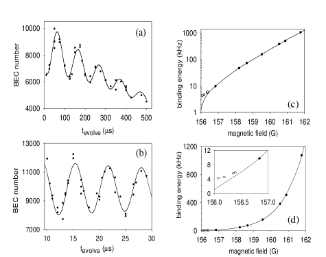
This is basically the idea of the Ramsey experiments performed by Donley et al. [69] and Claussen et al. [80]. Roughly speaking, the atomic condensate corresponds to oscillator and the molecular condensate to oscillator . Therefore, after performing the double-pulse sequence in the magnetic field one makes a light-absorption image of the atomic density from which one extracts the number of condensate and noncondensed atoms. Since this imaging technique is sensitive to a specific absorption line of the atoms it does not measure the number of molecules.
From the above discussion we expect to observe oscillations in the number of condensate atoms. Moreover, if the situation is such that the detuning between the pulses is relatively large the effect of the coupling can be neglected and the frequency of the observed oscillations corresponds to the energy difference between the atoms and the molecules, i.e., the molecular binding energy. This is indeed what is observed, thereby providing compelling evidence for the existence of coherence between atoms and molecules.
In Fig. 26 the experimental results of Claussen et al. [80] are presented. Fig. 26 (a) and (b) show the number of atoms in the atomic Bose-Einstein condensate as a function of after a double-pulse sequence. Clearly, there is an oscillation in the number of atoms in both cases. In Fig. 26 (a) the magnetic field between the pulses is G. In Fig. 26 (b) we have G which is further from resonance. This explains also the increase in frequency from (a) to (b) since further from resonance the molecular binding energy is larger.
What is also observed is that there is a damping of the oscillations and an overall loss of condensate atoms. Experimentally, the number of atoms in the condensate is fit to the formula
| (297) |
where is the average number of condensate atoms, and are the oscillation amplitude and phase, respectively, and is the damping rate of the oscillations. The overall atom loss is characterized by a rate constant . The experimentally observed frequency is equal to . By defining the frequency of the coherent atom-molecule oscillation in this way one compensates for the effects of the damping on the frequency. For the results in Fig. 26 (a) we have that kHz and atom/s. The frequency is equal to kHz. For Fig. 26 (b) the frequency is equal to kHz. The damping and loss rate are negligible for the short time used to determine the frequency. It is found experimentally that both the damping rate and the loss rate increase as approaches the resonant value.
In Fig. 26 (c) and (d) the results for the frequency as a function of are presented. The solid line shows the result of a two-body coupled-channels calculation of the molecular binding energy [80]. The parameters of the interatomic potentials are fit to the experimental results for the frequency. Clearly, the frequency of the coherent atom-molecule oscillations agrees very well with the molecular binding energy in vacuum over a large range of the magnetic field. Moreover, in the magnetic-field range G the frequency of the oscillations is well described by the formula for the binding energy, derived in Section 4.1.2. Close to resonance, however, the measured frequency deviates from the two-body result. The deviating experimental points are shown by open circles and are not taken into account in the determination of the interatomic potential. This deviation is due to many-body effects [81].
Although some of the physics of these coherent atom-molecule oscillations can roughly be understood by a simple two-level picture, it is worth noting that the physics of a Feshbach resonance is much richer. First of all, during Rabi oscillations in a simple two-level system one quantum in a state oscillates to the other state. In the case of a Feshbach resonance pairs of atoms oscillate back and forth between the dressed-molecular condensate and the atomic condensate. Therefore, the hamiltonian is not quadratic in the annihilation and creation operators and the physics is more complicated. In particular the dressed molecule may decay into two noncondensed atoms instead of forming two condensate atoms. This process is discuss in detail below. Second, the observed atom-molecule oscillations are oscillations between an atomic condensate and a dressed molecular condensate. The fact that one of the levels is a dressed molecule implies that by changing the magnetic field not only the detuning is altered, but also the internal state of the molecule itself.
This is seen most easily by considering the linearized version of the time-dependent mean-field equation in Eq. (5.1.2). Writing and , we have that
| (298) |
where we neglected the off-resonant part of the interatomic interactions. This is justified sufficiently close to resonance, where we are also allowed to neglect the energy-dependence of the atom-molecule coupling constant.
Consider first the situation that the fractional derivative is absent in the linearized mean-field equations in Eq. (6.1), i.e., we are dealing with the model of Drummond et. al. [70], and Timmermans et al. [71, 83]. These coupled equations describe exactly the same Rabi oscillations as the coupled harmonic oscillators in Eq. (291), with the coupling equal to . In the context of particle-number oscillations between condensates, Rabi oscillations are referred to as Josephson oscillations and the associated frequency is called the Josephson frequency. The Josephson frequency in the absence of the fractional derivative term in Eq. (6.1) is given by
| (299) |
which reduces to sufficiently far off resonance where the coupling may be neglected. This result does not agree with the experimental result because, by neglecting the fractional derivative, which corresponds to the molecular self-energy, we are describing Josephson oscillations between an atomic condensate and a condensate of bare molecules instead of dressed molecules. Furthermore, using the result in Eq. (292) we have that the amplitude of these oscillations is given by
| (300) |
In first approximation we take the dressing of the molecules into account as follows. If we are in the magnetic-field range where the Josephson frequency deviates not too much from the molecular binding energy, we are allowed to expand the propagator of the molecules around the pole at the bound-state energy. As we have seen in Section 4.1.3 this corresponds to introducing the dressed molecular field and leads to the Heisenberg equations of motion in Eq. (4.1.3). The linearized mean-field equations that describe the Josephson oscillations of a atomic and a dressed-molecular condensate are therefore given by
| (301) |
and lead to the Josephson frequency
| (302) |
which reduces to in the situation where the coupling is much smaller than the binding energy. This result agrees with the experimental fact that the measured frequency is, sufficiently far from resonance, equal to the molecular binding energy. Moreover, the initial deviation from the two-body result in the measured frequency is approximately described by the equation for the Josephson frequency in Eq. (302). The amplitude of the oscillations is in this case given by
| (303) |
which close to resonance is much larger than the result in Eq. (300).
To get more quantitative understanding of the magnetic-field dependence of the Josephson frequency over the entire experimentally investigated range of magnetic field we calculate this frequency in a linear-response approximation, including the energy-dependence of the atom-molecule coupling and the atom-atom interactions.
Before doing so, we make some remarks about the origin of the damping of the coherent atom-molecule oscillations and the overall loss of atoms that is observed in the experiments. One contribution to the damping is expected to be due to rogue dissociation [78]. Physically, this process corresponds to a pair of condensate atoms forming a dressed condensate molecule that then breaks up into two noncondensed atoms instead of oscillating back to the atomic condensate. This process is incorporated into our theory by the imaginary part of the molecular self-energy. As explained in Section 4.1.3 in the derivation of the Heisenberg equations of motion in Eq. (4.1.3), that involve the dressed molecules, we have neglected such a process. It is, however, incorporated in the full solution of the mean-field equation in Eq. (5.1.2). In the last section of the section we present the results of numerical solutions of these equations.
The overall loss of atoms from the atomic condensate is also partially due to the rogue-dissociation process. The experimental fact that a significant thermal component is formed during the double-pulse sequence supports this idea. Apart from this process, it may also be that conventional loss processes, such as dipolar decay and three-body recombination play a role. Although such processes are expected to become more important near a Feshbach resonance, they are, however, not included in our simulations since there is no detailed knowledge about the precise magnetic-field dependence near the resonance. In principle, however, these loss processes could be straightforwardly included in our calculations, by adding the appropriate imaginary terms to the mean-field equations. Another possible mechanism is the loss of atoms due to elastic collisions, the so-called quantum evaporation process [41]. This process is also not included in our present calculations.
6.2 Josephson frequency

With the mean-field theory derived in the previous sections we now calculate the magnetic-field and density dependence of the Josephson frequency of the coherent atom-molecule oscillations, in a linear approximation. The only parameter that has not been determined yet is the effective range of the interatomic interactions . All other parameters are known for 85Rb.
The effective range is determined by calculating the molecular binding energy in vacuum and comparing the result with the experimental data. We have seen that far off resonance the Josephson frequency is essentially equal to the molecular binding energy. Since the effect of a nonzero effective range only plays a role for large energies, and thus is important far off resonance, this comparison uniquely determines the effective range. As explained in detail in Section 4.1.2, the molecular binding energy is determined by solving for in the equation
| (304) |
For 85Rb the background scattering length is negative and the effective range turns out to be positive. The retarded molecular self-energy is therefore given by
| (305) |
In Fig. 27 the result of the numerical solution of Eq. (304) is shown for . Also shown in this figure are the experimental data points. Clearly, far off resonance there is good agreement between our results and the experimental data points. Therefore, we use this value for the effective range from now on in all our calculations. The absolute value of the detuning is shown by the dotted line, and deviates significantly from the binding energy. The dashed line in Fig. 27 indicates the formula . As we have derived in Section 4.1.2 this formula should accurately describe the magnetic-field dependence of the binding energy close to resonance. Clearly, the solid line that indicates the result that includes the nonzero effective range becomes closer to the dashed line as we approach resonance. However, there is a significant range of magnetic field where we need to include the effective range in our calculations. Closer to the resonance, the experimental points start to deviate from the two-atom binding energy. This deviation is taken into account by considering many-body effects. Note, therefore, that the expected oscillation frequency never leads to a quantitative agreement with experiment.

As mentioned previously, we calculate the many-body effects on the frequency of the coherent atom-molecule oscillations in linear approximation. Therefore, we first need to determine the equilibrium around which to linearize. In detail, the equilibrium values of the atomic and molecular condensate wave functions are determined by solving the time-independent mean-field equations in Eq. (5.1.1) together with the equation for the Hartree-Fock self-energy in Eq. (236) at a fixed chemical potential . To compare with the experimental results it is more convenient to solve these equations at a fixed condensate density. The chemical potential is then determined from these equations.
In Fig. 28 we show the result of this calculation for an atomic condensate density of cm-3. The solid line shows the Hartree-Fock self-energy and the dashed line the chemical potential as a function of the magnetic field, both in units of the energy . Note that far off resonance, where the energy dependence of the interaction may be neglected, we have that and . This is the expected result. The inset of Fig. 28 shows the fraction of bare molecules . Note that this fraction is always very small. This justifies neglecting the atom-molecule and molecule-molecule interactions since from this figure we see that the mean-field energies associated with these interactions are at least three orders of magnitude smaller. A posteriori this observation justifies neglecting the effect of the presence of the molecular condensate on the atoms in the approach of Köhler et al. [84].

Since the coherent atom-molecule oscillations are a collective mode where the amplitude of the atomic and molecular condensate wave functions oscillate out-of-phase, we study the collective modes of the system. As explained in detail in the previous section, the frequencies of the collective modes are determined by Eq. (260). This equation is solved numerically and yields a dispersion relation with two branches.
The result of this calculation is shown in Fig. 29 for an atomic condensate density of cm-3 and a magnetic field of G. The momentum is indicated in units of the inverse coherence length . The upper branch corresponds to the gapless phonon excitations. For small momenta this branch has a linear momentum dependence. The upper dashed line indicates the Bogoliubov dispersion in Eq. (252) evaluated at the scattering length . For small momentum the solid and the dashed line are almost identical. For larger momenta the numerically exact result is smaller, due to the energy-dependence of the interactions that effectively reduce the scattering length.

The lower branch corresponds to the coherent atom-molecule oscillations and is gapped. The solid line indicates the result of the full calculations. For small momenta it is well described by
| (306) |
where is the Josephson frequency. The dispersion resulting from this last equation is shown in the lower part Fig. 29 by the dashed line. This momentum dependence is to be expected since sufficiently far from resonance the atom-molecule oscillations reduce to a two-body excitation. The fact that the dispersion is negative is due to the fact that we are linearizing around a metastable situation with more atoms than molecules. Although this is the experimentally relevant situation, the true equilibrium situation for negative detuning corresponds to almost all atoms in the molecular state [83].
In Fig. 30 we present the results for the Josephson frequency as a function of the magnetic field, for different values of the condensate density. The solid lines in this figure show, from top to bottom, the results for an decreasing nonzero condensate density. The respective condensate densities are given by cm-3, cm-3, and cm-3. The dashed line shows the molecular binding energy in vacuum. The Josephson frequency reduces to the molecular binding energy for all values of the condensate density, in agreement with previous remarks. Nevertheless, sufficiently close to resonance there is a deviation from the two-body result due to many-body effects. This deviation becomes larger with increasing condensate density.
In order to confront our results with the experimental data we have to realize that the experiments are performed in a magnetic trap. Taking only the ground states and into account for both the atomic and the molecular condensates, respectively, this implies effectively that the atom-molecule coupling is reduced by an overlap integral. Hence we define the effective homogeneous condensate density by means of , where denotes the number of condensed atoms and and the radial and axial trapping frequencies, respectively. For the experiments of Claussen et al. we have that during the oscillations close to resonance as seen from Fig. 26, which results in an effective density of cm-3. This agrees also with the effective homogeneous density quoted by Claussen et al. [80]. The solid curve in Fig. 30 clearly shows an excellent agreement with the experimentally observed frequency for this density.
It is important to note that there are two hidden assumptions in the above comparison. First, we have used that the dressed molecules are trapped in the same external potential as the atoms. This is not obvious because the bare molecular state involved in the Feshbach resonance is high-field seeking and therefore not trapped. However, Eq. (183) shows that near resonance almost all the amplitude of the dressed molecule is in the low-field seeking open channel and its magnetic moment is therefore almost equal to twice the atomic magnetic moment. Second, we have determined the frequency of the coherent atom-molecule oscillations in equilibrium. In contrast, the observed oscillations in the number of condensate atoms is clearly a nonequilibrium phenomenon. This is, however, expected not to play an important role because the Ramsey-pulse sequence is performed on such a fast time scale that the response of the condensate wave function can be neglected. By variationally solving the Gross-Pitaevskii equation for the atomic condensate wave function, we have explicitly checked that after a typical pulse sequence its width is only a few percent larger than the harmonic oscillator ground state.

Finally, we calculate the Josephson frequency as a function of the condensate density. The results of this calculation are presented in Fig. 31, for various values of the magnetic field which is kept fixed in these calculations. In the presentation of the results we have subtracted the molecular binding energy to bring out the many-body effects more clearly. As expected, the difference between the Josephson frequency and the molecular binding energy increases with increasing condensate density. Moreover, for values of the magnetic field closer to resonance the difference is also larger.
The above calculations in the linear approximation give already a great deal of insight in the coherent atom-molecule oscillations, and, in particular, in their many-body aspects. In the next section we aim at achieving also insight in the nonlinear dynamics and damping resulting from the time-dependent mean-field equations for the double-pulse experiments. In particular, we also discuss the rogue-dissociation process. The nonlinear effects in these experiments has first been discussed by Kokkelmans and Holland [79], Mackie et al. [78], and Köhler et al. [84], on the basis of their mean-field approaches summarized in Section 5.2.
6.3 Beyond linear response

In this section we discuss the numerical solution of the time-dependent mean-field equations using the methods described in Sec. 5.1.2. We focus here on the situation where the detuning is only changed instantaneously, so that we are allowed to use the Green’s function method discussed in this section. After the elimination of the molecular condensate wave function from the mean-field equations, the effective equation for the atomic condensate wave function is then given by
| (307) |
In this equation, the term that involves the integral over frequencies describes the fact that a pair of condensate atoms that forms a molecule can decay into a pair of noncondensed atoms with opposite momenta, i.e., the rogue-dissociation process. In the absence of this term the equation effectively takes into account the dressing of molecules in an adiabatic manner, and describes Josephson oscillations between a condensate of atoms and dressed molecules.
As we have discussed in the previous section, the above equation is only applicable to the situation of a sudden change in magnetic field. Therefore, we perform the following calculation. For a given magnetic field and atomic condensate density we calculate the equilibrium values of the molecular wave functions and the Hartree-Fock self-energy, using the time-independent mean-field equations in Eq. (5.1.1) and Eq. (236). Then we change the magnetic field instantaneously to the value and keep it at this value. In Fig. 32 the results of the calculations for this situation are shown, with G and G. The atomic condensate density is taken equal to cm-3. The dashed line shows the result for a calculation without the rogue-dissociation process and shows oscillations where a fraction of the atoms is converted into molecules and oscillates back and forth between the atomic and dressed molecular condensate. Since there is no decay mechanism, all of the atoms come back into the atomic condensate at times equal to a multiple of the oscillation period. The solid line shows the result of a calculation that includes the rogue-dissociation process. Clearly, the number of condensate atoms oscillates in this case as well. However, not all of the atoms come back into the atomic condensate and there is a decay of the number of atoms in the atomic condensate. This is precisely due to the above-mentioned rogue-dissociation process.
Although the preliminary calculations presented in this section are limited to the case of a step in the magnetic field, they nevertheless present some insight in the effects of the rogue-dissociation process on the coherent atom-molecule oscillations in a Ramsey experiment. In future work we intend to study also the case of time-dependent magnetic fields, by an exact numerical treatment of the fractional derivative in our time-dependent mean-field equations. In particular, we are interested in the magnetic-field dependence of the damping that is caused by the rogue-dissociation process.
We can estimate this dependence as follows. The Green’s function associated with the rogue-dissociation process,
| (308) |
is sharply peaked in time. Hence we approximate this Green’s function by
| (309) |
with the timescale given by
| (310) |
with a positive cut-off that is determined such that the result for depends only very weakly on . The Green’s function evaluated at zero time equals , a result which follows from the sum rule for the molecular density of states in Eq. (182). This gives the contribution
| (311) |
to the right-hand side of Eq. (6.3). The rate equation for the atomic density that follows from this term is given by
| (312) |
which after linearization leads to the following equation for the number of condensate atoms
| (313) |
with the rate given by
| (314) |
We observe from this equation that the loss rate of atoms from the atomic condensate due to the rogue-dissociation process increases as the magnetic field approaches its resonant value. This is indeed what is observed experimentally [80]. Far off resonance the loss rate vanishes since the wave function renormalization factor in this limit. For the parameters of Fig. 26 (a) at the effective homogeneous density cm-3, we have that s, which leads to kHz. The dotted line in Fig. 32 shows the result of a calculation that includes the term in Eq. (311). The exact result, shown by the solid line, and this approximate result show the same overall damping rate. This justifies the approximation for the Green’s function in Eq. (309). The result for the damping rate is about a factor of eight smaller than the experimental result.

To further investigate the magnetic-field dependence of the damping of the coherent atom-molecule oscillations, we have calculated the numerical solution of the effective equation of motion for the atomic condensate wave function for a step in the magnetic field, for three different final magnetic fields. The results of these calculations are shown in Fig. 33. The solid, dashed, and dotted lines corresponds to a magnetic field of G, G, and G, respectively. The initial equilibrium corresponds to an atomic condensate density of cm-3 at a magnetic field of G. Note the increase in the frequency with increasing magnetic field.
The magnetic-field dependence of the frequency and damping of the coherent atom-molecule oscillations is found from these numerical results by fitting with the equation in Eq. (297). The results are presented in Fig. 34. The solid line corresponds to the Josephson frequency of the coherent atom-molecule oscillations that was found by means of the linear-response calculation of the previous section. The deviation for large magnetic fields is understood because we have, in our numerical solution of the effective mean-field equation, not taken into account the higher-order energy-dependences of the molecular self-energy that are fully taken into account in the linear-response theory. The inset shows the damping as a function of the magnetic field. Note the increase of the damping as the magnetic field approaches its resonant value. This is expected from the estimate in Eq. (314).

The above analysis indicates that the rogue-dissociation process gives possibly a contribution to the experimentally observed damping of the coherent atom-molecule oscillations. Presumably, however, also other mechanisms contribute to the observed damping. In particular, we mention here the quantum evaporation process, that was shown to be important in the single-pulse experiments [41]. The detailed investigation of the damping of the coherent atom-molecule oscillation is a subject for further study.
7 Conclusions and outlook
In this review paper we have presented the derivation of an effective quantum field theory suitable for the description of a Bose gas near a Feshbach resonance, since it incorporates the two-atom physics exactly. We have presented several applications of this theory, both above and below the critical temperature for Bose-Einstein condensation. In the last part of this paper we have studied in detail the magnetic-field dependence of the frequency of the coherent atom-molecule oscillations and have obtained excellent agreement with the experimental results. In particular, we have been able to quantitatively explain the many-body effects on this frequency by making use of a linear-response approximation to our mean-field equations. Although we have already presented some numerical solutions of the mean-field equations that improve on this approximation, a great deal of work still has to be done. The numerical solution of these equations for the situation of time-dependent detuning is rather involved. Nevertheless, work in this direction is in progress and will be reported in a future publication.
As already mentioned, we have also discussed the properties of the gas above the critical temperature. This discussion was mainly concerned with the equilibrium properties of the gas and we studied the many-body effects on the bound-state energy of the molecular state. An important conclusion of this study is that, for certain values of the parameters, there exists a many-body induced resonant state with a relatively small energy. In future work we intend to study the effects of the appearance of this resonant state in the molecular density of states on the properties of the gas. In particular we expect that due to this effect the number of molecules in the gas will be large even at relatively large detuning, which can not be explained on the basis of two-atom physics.
Furthermore, to study the normal state also in an out-of-equilibrium situation, we should derive a quantum kinetic theory that describes the evolution of the local occupation numbers of the atoms and molecules. Moreover, the description of the Bose-Einstein condensed phase of the gas at nonzero temperatures requires a modification of the mean-field equations such that they include the effects of the thermal clouds of atoms and molecules, and we need equations for the evolution of the local occupation numbers of the latter. The extension of the theory presented in this paper to these situations can be derived in a unifying manner by using a functional formulation of the Schwinger-Keldysh nonequilibrium theory [113], and is especially important in view of the ongoing effort to produce ultracold molecules by means of a sweep in the magnetic field through the Feshbach resonance [62].
The theory presented in this paper is generalized to a gas of fermionic atoms in a straightforward manner [68, 85]. One modification is that to have -wave scattering between fermionic atoms we have to have a mixture of atoms with two hyperfine states, since the Pauli principle forbids -wave scattering between identical fermions. Furthermore, the properties of the dressed molecular state is altered due to the presence of the Fermi sphere. A molecule with zero momentum only decays if its energy is above twice the Fermi energy. If the molecular state lies below twice the Fermi energy, the equilibrium situation is a Bose-Einstein condensate of molecules. If we start from this situation and increase the detuning, the Bose-Einstein condensate of molecules crosses over to a Bose-Einstein condensate of Cooper pairs, i.e., a BCS-BEC crossover occurs [61, 57]. In view of the ongoing experiments with atomic Fermi gases near a Feshbach resonance [62, 63, 64, 65, 66, 67], it is particularly interesting to study the effects of nonadiabticity on the crossover from a Bose-Einstein condensate of molecules to a degenerate Fermi gas. In particular, the atomic distribution function after such a sweep, and its dependence on the duration of the sweep, is of great interest, since this will determine whether or not a BCS-state will form after equilibration. Determination of the atomic distribution function requires, in first instance, knowledge of the solution of the mean-field equation for the molecular condensate for time-dependent detuning. Work in this direction is in progress. We also intend to study the equilibrium properties of this crossover, and in particular the behaviour of the critical temperature, in detail in future work.
Clearly, Feshbach resonances present an exciting opportunity for the experimental and theoretical study of the many-body properties of atomic and molecular Bose and Fermi gases. There is little doubt that these Feshbach resonances will find many new applications in the years to come.
References
- [1] M.H. Anderson, J.R. Ensher, M.R. Matthews, C.E. Wieman, and E.A. Cornell, Science 269, 198 (1995).
- [2] S. Giorgini, L.P. Pitaevskii, and S. Stringari, Rev. Mod. Phys. 71, 463 (1999).
- [3] A.J. Leggett, Rev. Mod. Phys. 73, 307 (2001).
- [4] C.J. Pethick and H. Smith, Bose-Einstein Condensation in Dilute Gases (Cambridge University Press, Cambridge, 2002).
- [5] L.P. Pitaevskii and S. Stringari, Bose-Einstein Condensation (Oxford University Press, Oxford, 2003).
- [6] S. Inouye, M.R. Andrews, J. Stenger, H.-J. Miesner, D.M. Stamper-Kurn, and W. Ketterle, Nature 392, 151 (1998).
- [7] H. Feshbach, Ann. Phys. 19, 287 (1962).
- [8] F.S. Levin and H. Feshbach, Reaction Dynamics (Gordon and Breach, New York, 1973).
- [9] W.C. Stwalley, Phys. Rev. Lett. 37, 1628 (1976).
- [10] E. Tiesinga, B.J. Verhaar, and H.T.C. Stoof, Phys. Rev. A 47, 4114 (1993).
- [11] Ph. Courteille, R.S. Freeland, D.J. Heinzen, F.A. van Abeelen, and B.J. Verhaar, Phys. Rev. Lett. 81, 69 (1998).
- [12] J.L. Roberts, N.R. Claussen, J.P. Burke, Jr., C.H. Greene, E.A. Cornell, and C.E. Wieman, Phys. Rev. Lett. 81, 5109 (1998).
- [13] V. Vuletić, A.J. Kerman, C. Chin, and S. Chu, Phys. Rev. Lett. 82, 1406 (1999).
- [14] A. Marte, T. Volz, J. Schuster, S. Dürr, G. Rempe, E. G. M. van Kempen, and B. J. Verhaar, Phys. Rev. Lett. 89, 283202 (2002).
- [15] K.S. Strecker, G.B. Partridge, A.G. Truscott, and R.G Hulet, Nature 417, 150 (2002).
- [16] K. Dieckmann, C. A. Stan, S. Gupta, Z. Hadzibabic, C. H. Schunck, and W. Ketterle, Phys. Rev. Lett. 89, 203201 (2002).
- [17] K.M. O’Hara, S.L. Hemmer, M.E. Gehm, S.R. Granade, and J.E. Thomas, Science 298, 2179 (2002).
- [18] C.A. Regal and D.S. Jin, Phys. Rev. Lett. 90, 230404 (2003).
- [19] T. Bourdel, J. Cubizolles, L. Khaykovich, K. M. F. Magalhaes, S. J. J. M. F. Kokkelmans, G. V. Shlyapnikov, and C. Salomon, Phys. Rev. Lett. 91, 020402 (2003).
- [20] P.A. Ruprecht, M.J. Holland, K. Burnett, and M. Edwards, Phys. Rev. A 51, 4704 (1995).
- [21] E.V. Shuryak, Phys. Rev. A 54, 3151 (1996).
- [22] H.T.C. Stoof, J. Stat. Phys. 87, 1353 (1997).
- [23] M. Houbiers and H.T.C. Stoof, Phys. Rev. A 54, 5055 (1996).
- [24] T. Bergeman, Phys. Rev. A 55, 3658 (1997).
- [25] C.C. Bradley, C.A. Sackett, J.J. Tollett, and R.G. Hulet, Phys. Rev. Lett. 75, 1687 (1995); C.C. Bradley, C.A. Sackett, and R.G. Hulet, Phys. Rev. Lett. 78, 985 (1997).
- [26] R.A. Duine and H.T.C. Stoof, Phys. Rev. A 65, 013603 (2002).
- [27] C.A. Sackett, H.T.C. Stoof, and R.G. Hulet, Phys. Rev. Lett. 80, 2031 (1998).
- [28] C.A. Sackett, J.M. Gerton, M. Welling, and R.G. Hulet, Phys. Rev. Lett. 82, 876 (1999).
- [29] J.M. Gerton, D. Strekalov, I. Prodan, and R.G. Hulet, Nature 408, 692 (2000).
- [30] S.L. Cornish, N.R. Claussen, J.L. Roberts, E.A. Cornell, C.E. Wieman, Phys. Rev. Lett. 85, 1795 (2000).
- [31] J.L. Roberts, N.R. Claussen, S.L. Cornish, E.A. Donley, E.A. Cornell, and C.E. Wieman, Phys. Rev. Lett. 86, 4211 (2001).
- [32] E.A. Donley, N.R. Claussen, S.L. Cornish, J.L. Roberts, E.A. Cornell, and C.E. Wieman, Nature 412, 295 (2001).
- [33] Yu. Kagan, A.E. Muryshev, and G.V. Shlyapnikov, Phys. Rev. Lett. 81, 933 (1998).
- [34] M. Ueda and K. Huang, Phys. Rev. A 60, 3317 (1999).
- [35] A. Eleftheriou and K. Huang, Phys. Rev. A 61,43601 (2000).
- [36] S.K. Adhikari, Phys. Lett. A 296, 145 (2002); Phys. Rev. A 66, 013611 (2002).
- [37] H. Saito and M. Ueda, Phys. Rev. A 65, 033624 (2002).
- [38] L. Santos and G.V. Shlyapnikov, Phys. Rev. A 66, 011602(R) (2002).
- [39] W. Bao, D. Jaksch, and P.A. Markowich (cond-mat/0307344).
- [40] R.A. Duine and H.T.C. Stoof, Phys. Rev. Lett. 86, 2204 (2001).
- [41] R.A. Duine and H.T.C. Stoof, Phys. Rev. A 68, 013602 (2003).
- [42] J. N. Milstein, C. Menotti, and M. J. Holland, New. J. Phys. 5, 52 (2003).
- [43] U. Al Khawaja, H. T. C. Stoof, R. G. Hulet, K. E. Strecker, and G. B. Partridge, Phys. Rev. Lett. 89, 200404 (2002).
- [44] W.J. Mullin, J. Low. Temp. Phys. 106, 615 (1997).
- [45] T-L. Ho and M. Ma, J. Low. Temp. Phys. 115, 61 (1999).
- [46] D.S. Petrov, M. Holzmann, and G.V. Shlyapnikov, Phys. Rev. Lett. 84, 2551 (2000).
- [47] D.S. Petrov, G.V. Shlyapnikov, and J.T.M. Walraven, Phys. Rev. Lett. 85, 3745 (2000).
- [48] D.S. Petrov, G.V. Shlyapnikov, and J.T.M. Walraven, Phys. Rev. Lett. 87, 050404 (2001).
- [49] J.O. Andersen, U. Al Khawaja, and H.T.C. Stoof, Phys. Rev. Lett. 88, 070407 (2002).
- [50] L. Khaykovich, F. Schreck, G. Ferrari, T. Bourdel, J. Cubizolles, L. D. Carr, Y. Castin, and C. Salomon, Science 296, 1290 (2002).
- [51] H. T. C. Stoof, M. Houbiers, C. A. Sackett, and R. G. Hulet, Phys. Rev. Lett. 76, 10 (1996); M. Houbiers, R. Ferwerda, H.T.C. Stoof, W.I. McAlexander, C.A. Sackett, and R.G. Hulet, Phys. Rev. A 56, 4864 (1997).
- [52] M. Holland, S. J. J. M. F. Kokkelmans, M. L. Chiofalo, and R. Walser, Phys. Rev. Lett. 87, 120406 (2001).
- [53] S.J.J.M.F. Kokkelmans, J.N. Milstein, M.L. Chiofalo, R. Walser, and M.J. Holland, Phys. Rev. A 65, 053617 (2002).
- [54] J.N. Milstein, S.J.J.M.F. Kokkelmans and M.J. Holland, Phys. Rev. A 66, 043604 (2002).
- [55] Y. Ohashi and A. Griffin, Phys. Rev. Lett. 89, 130402 (2002).
- [56] Y. Ohashi and A. Griffin, Phys. Rev. A 67, 033603 (2003).
- [57] Y. Ohashi and A. Griffin, Phys. Rev. A 67, 063612 (2003).
- [58] R. Combescot, New. J. Phys. 5, 86 (2003).
- [59] R. Combescot, Phys. Rev. Lett. 83, 3766 (1999).
- [60] H. Heiselberg, C. J. Pethick, H. Smith, and L. Viverit, Phys. Rev. Lett. 85, 2418 (2000).
- [61] P. Nozières and S. Schmitt-Rink, J. Low. Temp. Phys. 59, 195 (1985).
- [62] C. A. Regal, C. Ticknor, J. L. Bohn, and D.S. Jin, Nature 424, 47 (2003).
- [63] K. E. Strecker, G. B. Partridge, and R. G. Hulet, Phys. Rev. Lett. 91, 080406 (2003).
- [64] K. Xu, T. Mukaiyama, J. R. Abo-Shaeer, J. K. Chin, D. E. Miller, and W. Ketterle, Phys. Rev. Lett. 91, 210402 (2003).
- [65] S. Jochim, M. Bartenstein, A. Altmeyer, G. Hendl, S. Riedl, C. Chin, J. Hecker Denschlag, and R. Grimm, Science.1093280 (2003).
- [66] M. Greiner, C. A. Regal, and D. S. Jin (cond-mat/0311172).
- [67] M.W. Zwierlein, C.A. Stan, C.H. Schunck, S.M.F. Raupach, S. Gupta, Z. Hadzibabic, W. Ketterle (cond-mat/0311617).
- [68] G.M. Falco, R.A. Duine and H.T.C. Stoof (cond-mat/0304489).
- [69] E.A. Donley, N.R. Claussen, S.T. Thompson, and C.E. Wieman, Nature 417, 529 (2002).
- [70] P.D. Drummond, K.V. Kheruntsyan, and H. He, Phys. Rev. Lett. 81, 3055 (1998).
- [71] E. Timmermans, P. Tommasini, R. Côté, M. Hussein and A. Kerman, Phys. Rev. Lett. 83, 2691 (1999).
- [72] N.R. Claussen, E.A. Donley, S.T. Thompson, and C.E. Wieman, Phys. Rev. Lett. 89, 010401 (2002).
- [73] A. J. Moerdijk, H. M. J. M. Boesten, and B. J. Verhaar, Phys. Rev. A 53, 916 (1996).
- [74] P. O. Fedichev, M. W. Reynolds, and G. V. Shlyapnikov, Phys. Rev. Lett. 77, 2921 (1996).
- [75] B. D. Esry, C. H. Greene, and J. P. Burke, Jr., Phys. Rev. Lett. 83, 1751 (1999).
- [76] E. Braaten and H.-W. Hammer, Phys. Rev. Lett. 87, 160407 (2001).
- [77] J.L. Roberts, N.R. Claussen, S.L. Cornish, and C.E. Wieman, Phys. Rev. Lett. 85, 728 (2000).
- [78] M. Mackie, K.-A. Suominen, and J. Javanainen, Phys. Rev. Lett. 89, 180403 (2002).
- [79] S.J.J.M.F. Kokkelmans and M.J. Holland, Phys. Rev. Lett. 89, 180401 (2002).
- [80] N.R. Claussen, S.J.J.M.F. Kokkelmans, S.T. Thompson, E.A. Donley, and C.E. Wieman, Phys. Rev. A 67, 060701(R) (2003).
- [81] R.A. Duine and H.T.C. Stoof, Phys. Rev. Lett. 91, 150405 (2003).
- [82] R.A. Duine and H.T.C. Stoof, New. J. Phys. 5, 69 (2003).
- [83] E. Timmermans, P. Tommasini, H. Hussein, and A. Kerman, Phys. Rep. 315, 199 (1999).
- [84] T. Köhler, T. Gasenzer, and K. Burnett, Phys. Rev. A 67, 013601 (2003).
- [85] R.A. Duine and H.T.C. Stoof, J. Opt. B: Quantum Semiclass. Opt. 5, S212 (2003).
- [86] K. V. Kheruntsyan and P. D. Drummond, Phys. Rev. A 58, 2488 (1998); Phys. Rev. A 58, R2676 (1998); Phys. Rev. A 61, 063816 (2000).
- [87] J. Calsamiglia, M. Mackie, and K.-A. Suominen, Phys. Rev. Lett. 87, 160403 (2001).
- [88] M. Mackie, Phys. Rev. A 66, 043613 (2002).
- [89] T. Köhler, T. Gasenzer, P. Julienne, and K. Burnett (cond-mat/0302082).
- [90] T. Köhler and K. Goral (cond-mat/0305060).
- [91] J.J. Sakurai, Modern Quantum Mechanics (Addison-Wesley, New-York, 1994).
- [92] B.H. Bransden and C.J. Joachain, Introduction to Quantum Mechanics (Longman Scientific & Technical, Harlow, 1989).
- [93] See, for instance, H. T. C. Stoof, L. P. H. de Goey, W. M. H. M. Rovers, P. S. M. Kop Jansen, and B. J. Verhaar, Phys. Rev. A 38, 1248 (1988).
- [94] A similar example is briefly discussed in Ref. [53]. A more formal treatment of a Feshbach resonance in atomic scattering is discussed in Ref. [83].
- [95] H. Kleinert, Fort. Phys. 26, 565 (1978) and references therein.
- [96] H.T.C. Stoof in Coherent Atomic Matter Waves, edited by R. Kaiser, C. Westbrook, and F. David, p. 219 (Springer, Berlin, 2001).
- [97] H.T.C. Stoof, M. Bijlsma, and M. Houbiers, J. Res. Natl. Inst. Stand. Technol. 101, 443 (1996).
- [98] K. M. O’Hara, S. L. Hemmer, S. R. Granade, M. E. Gehm, J. E. Thomas, V. Venturi, E. Tiesinga, and C. J. Williams, Phys. Rev. A 66, 041401 (2002).
- [99] J.W. Negele and H. Orland, Quantum Many-Particle Systems (Addison-Wesley, New York, 1988).
- [100] M. Bijlsma and H.T.C. Stoof, Phys. Rev. A 54, 5085 (1996).
- [101] E.G.M. van Kempen, S.J.J.M.F. Kokkelmans, D.J. Heinzen, and B.J. Verhaar, Phys. Rev. Lett. 88, 093201 (2002).
- [102] For the case of a fermionic gas near a Feshbach resonance, see Ref. [56] for a similar discussion.
- [103] See also S.J.J.M.F. Kokkelmans, G.V. Shlyapnikov, and C. Salomon (cond-mat/0308384).
- [104] S. Sachdev, private communication.
- [105] M.W.J. Romans, R.A. Duine, S. Sachdev, and H.T.C. Stoof, to appear.
- [106] C. Chin, A. J. Kerman, V. Vuletić, and S. Chu, Phys. Rev. Lett. 90, 033201 (2003).
- [107] J. Goldstone, Nuova Cimento 19, 154 (1961).
- [108] N.N. Bogoliubov, J. Phys. (Moscow) 11, 23 (1947).
- [109] R. Hilfer, Applications of Fractional Calculus in Physics (World Scientific, Singapore, 2000).
- [110] N.P. Proukakis and K. Burnett, J. Res. Nat. Inst. Stand. Technol. 101, 457 (1996).
- [111] N.P. Proukakis, K. Burnett, and H.T.C. Stoof, Phys. Rev. A 57, 1230 (1998).
- [112] M. Bijlsma and H.T.C. Stoof, Phys. Rev. A 55, 498 (1997).
- [113] H.T.C. Stoof, J. Low Temp. Phys. 114, 11 (1999).