High Order Perturbation Theory for Spectral Densities of Multi-Particle Excitations: $\mathbf{S=\frac{1}{2}}$ Two-Leg Heisenberg Ladder

Abstract

We present a high order perturbation approach to quantitatively calculate spectral densities in three distinct steps starting from the model Hamiltonian and the observables of interest. The approach is based on the perturbative continuous unitary transformation introduced previously. It is conceived to work particularly well in models allowing a clear identification of the elementary excitations above the ground state. These are then viewed as quasi-particles above the vacuum. The article focuses on the technical aspects and includes a discussion of series extrapolation schemes. The strength of the method is demonstrated for $S=1/2$ two-leg Heisenberg ladders, for which results are presented.

I A. Introduction

Spectroscopic measurements provide important insights in the microscopic structure of solids. Generic spectroscopic data contains information about energy bands, associated density of states, matrix elements and selection rules. From the theoretical point of view this information is indispensable in the process of formulating and testing appropriate microscopic models. However, a quantitative comparison of the theoretical and the experimental data strongly depends on the power of the method used to calculate the properties of the microscopic model. In this context high order perturbation theory has proven to be a versatile and flexible tool. Especially in the field of spin models a variety of perturbation techniques is in use (for an overview see Ref. [1]). Most of them concentrate on the calculation of one-particle energies and in some circumstances on the associated spectral weights [2, 3, 4]. However, so far the important information contained in the line shapes of spectroscopic data, i.e., the model’s spectral densities associated with the experimental observables, has not been exploited. The need for a quantitative calculational tool closing this gap is apparent.

In the last couple of years there has been considerable progress in the field of high order perturbation theory. For a long time the methods were restricted to ground state energies and one-particle energies. Just recently we were able to quantitatively calculate two-particle excitation energies (bound states) in various spin models [5, 6]. These calculations were based on the perturbative continuous unitary transformation (CUT) method introduced previously [7]. This technique was used successfully for low-energy calculations in various spin models before [7, 8, 9]. The key point is to construct the transformation such that the resulting effective Hamiltonian is block-diagonal with respect to the number of particles. The linked cluster series expansion, an established high order perturbation method, has been shown lately to be also well suited for calculating two-particle energies [10, 11]. The basic idea is again the application of an orthogonal transformation which is designed to achieve a block-diagonal effective Hamiltonian.

In Ref. [12] we presented an extension of the CUT method allowing a systematic high order perturbation theory for observables. In the present article we use the results of Ref. [12] to calculate spectral densities of multi-particle excitations quantitatively. The method allows to obtain the complete spectral information for experimental relevant observables without any finite size restrictions. The results are exact in the sense of the thermodynamic limit, i.e., each order can be calculated for the thermodynamic limit. By truncating the series expansion at a (high) maximum order we restrict to dynamic processes for which the involved particles interact within a certain finite distance to each other. Obtaining higher orders amounts to allowing larger distances. Hence, the scheme can be expected to work particularly well in systems with short correlation lengths.

Results for various spin systems have been reported in earlier publications (Refs. [13, 14, 15, 16, 17, 18, 19, 20, 21]). The article on hand gives the technical details necessary to apply the method. We like to mention that the linked cluster method mentioned above was recently extended to allow for calculating spectral densities, too [22]. It thus constitutes an alternative approach.

To illustrate our approach we consider the $S=1/2$ antiferromagnetic two-leg Heisenberg ladder as an interesting and comprehensive testing ground. The Hamiltonian reads

$$H (J_{\perp},J_{\parallel})=J_{\perp}H_{\perp}+J_{\parallel}H_{\parallel}$$ (1)

$$= \sum_{i}\left[J_{\perp}{\mathbf{S}}_{1,i}{\mathbf{S}}_{2,i}\!+\!\!\!\ J_{\parallel}\left({\mathbf{S}}_{1,i}{\mathbf{S}}_{1,i+1}+{\mathbf{S}}_{2,i}{\mathbf{S}}_{2,i+1}\right)\right]\ ,$$ (2)

where $i$ denotes the rung and $1,2$ the leg.

In the broad field of spin liquid systems there has been an ongoing theoretical interest in the spin ladder and its extended versions [23, 24, 25, 26, 27, 28, 29, 30, 31, 32, 33, 34, 35, 36, 37, 11, 38]. The model is realized in a number of substances [39] and there is a large amount of experimental data available, see e.g. Refs. [40, 41, 42, 43, 44, 45, 46, 47]. Additionally, the experimental evidence for superconductivity in Sr_0.4Ca_13.6Cu₂₄O_41.84 under pressure [48] has intensified the interest.

I B. Article Outline

The basic concept of our approach to spectral densities is as follows. For a given observable $\mathcal{O}$ the $T=0$ spectral density is calculated from

$${\mathcal{S}}(\omega)=-\frac{1}{\pi}{\rm Im}{\mathcal{G}}(\omega)\ ,$$ (3)

where ${\mathcal{G}}(\omega)$ is the retarded zero temperature Green function

$${\mathcal{G}}(\omega)=\langle\psi_{0}|{\mathcal{O}}^{\dagger}(\omega-(H-E_{0})+i0+)^{-1}{\mathcal{O}}|\psi_{0}\rangle\ .$$ (4)

Here $\psi_{0}$ is the ground state and $E_{0}$ is the ground state energy of the system. Since the expectation values of quantum mechanical observables do not change under unitary transformations, the Green function ${\mathcal{G}}$, and thus ${\mathcal{S}}$, will not be altered if the operators $H$ and ${\mathcal{O}}$ and the state $|\psi_{0}\rangle$ appearing in ${\mathcal{G}}$ are substituted by the effective operators (state) $H_{\rm eff}$ and ${\mathcal{O}}_{\rm eff}$ ($|\psi_{0,\rm eff}\rangle$) obtained from the CUT method. Our procedure can be divided into three steps:

1. Use the CUT to derive an effective Hamiltonian $H_{\rm eff}$ unitarily linked to $H$.
   

2. Use the same transformation to derive the effective observable ${\mathcal{O}}_{\rm eff}$ from some initial observable ${\mathcal{O}}$ of interest.
   

3. Evaluate Eq. (4) for the effective operators in terms of a continued fraction.

Now, the key ingredient of our approach is to identify suitable (quasi-)particles which can be used to describe the $T=0$ physics of the system under study. We then proceed and construct the perturbative unitary transformation such that the resulting effective Hamiltonian $H_{\rm eff}$ conserves the number of these particles. Let $Q$ be the operator which counts the number of particles. Then the conservation of the number of quasi-particles reads

$$[H_{\rm eff},Q]=0\ .$$ (5)

In Sect. II we describe in detail how this idea can be put to use by illustrating the procedure for the spin ladder example.

Applying the same transformation to observables ${\mathcal{O}}$ different from the Hamiltonian leads to effective observables ${\mathcal{O}}_{\rm eff}$ not conserving the number of particles in general. Their action on the ground state, as needed in the evaluation of the Green function (4), is characterized by the number of particles they inject, i.e., by the number of elementary excitations they excite. We thus decompose ${\mathcal{O}}_{\rm eff}$ into operators injecting none, one, two and so on particles in the system. In Sect. III we again use the ladder example to illustrate the practical realization of this concept for experimentally relevant observables.

Once the effective Hamiltonian and the observables are obtained they are inserted into the Green function. Sect. IV features a detailed description of how the resulting expression is manipulated to extract the corresponding (energy- and momentum-resolved) spectral densities. Again, the one-, two- and more-particle contributions to the total spectral density can be treated separately leading to a simple and comprehensive physical picture in the end.

In Sect. V we address the problem of series extrapolation, an inevitable difficulty in perturbative approaches. Following our approach, a very large number of quantities has to be extrapolated simultaneously. This poses a difficulty which cannot always be tackled by standard techniques. We introduce a robust extrapolation scheme based on optimized perturbation theory [49] and show how it can be applied to extend the range of the perturbative results.

The article is summarized in Sect. VI.

II Transformation of the Hamiltonian

We start by briefly explaining how the effective Hamiltonian $H_{\rm eff}$ is constructed from the initial ladder Hamiltonian (1). (Other examples for this procedure can be found in Refs. [7, 9] for instance.) In the subsequent sections II.A through II.C we illustrate in detail how the zero-, one- and two-particle energies are calculated from $H_{\rm eff}$.

Let us assume that the initially given Hamiltonian $H$ can be formulated as perturbative problem

$$H=U+xV\ .$$ (6)

In its present formulation (extensions are possible) the perturbative CUT method relies on two prerequisites calling for a band-diagonal problem as starting point:

1. The unperturbed Hamiltonian U must have an equidistant spectrum bounded from below. The difference between two successive levels is called an energy quantum or (quasi-)particle and we identify $Q=U$.

2. There is a number ${\mathbb{N}}\ni N>0$ such that the perturbing Hamiltonian $V$ can be written as $V=\sum_{n=-N}^{N}T_{n}$ where $T_{n}$ increments (or decrements, if $n<0$) the number of energy quanta by $n$: $[Q,T_{n}]=nT_{n}$.

We now show that the initial ladder Hamiltonian (1) meets these requirements. We reformulate the ladder problem according to

$$\frac{H(x)}{J_{\perp}}=H_{\perp}+xH_{\parallel},$$ (7)

with $x=J_{\parallel}/J_{\perp}$ as perturbation parameter, $H_{\perp}=H(1,0)$ and $H_{\parallel}=H(0,1)$. We assume $J_{\perp}$ to be antiferromagnetic and set $J_{\perp}=1$ henceforth. The limit of isolated rungs is the limit for which our perturbative treatment is controlled.

The ground state of the unperturbed part $H_{\perp}$ is the product state with singlets on all rungs. A first excited state is a single rung excited to a triplet. There are $3L/2$ such elementary triplet excitations if $L$ is the number of spins. The energetically next higher state is given by two rung-triplets and so on. The operator $H_{\perp}$ simply counts the number of rung-triplets and it is easily verified that condition (A) is fulfilled.

For the rest of this article we identify $Q=H_{\perp}$, i.e., the elementary excitations of the unperturbed part (rung-triplets) serve as (quasi-)particles in our treatment of the ladder system. Since we prefer the particle picture we call these elementary excitations triplons [18]. They are total spin $S=1$ excitations appearing in three different variants ($S^{z}$-components -1,0,1) in contrast to magnons which have two variants only ($S^{z}\pm 1$) in a phase of broken spin symmetry. Both, triplons and magnons, must be distinguished from spinons, which are $S=1/2$ excitations. Whenever we refer to the ladder system we will use the term triplon. In more general discussions we retreat to the term (quasi-)particle.

As soon as we turn on the inter-rung interaction ($x>0$) the triplons become dressed particles. The central idea of the CUT approach is to map the initial problem onto an effective Hamiltonian for which the simple triplon-states, originally defined for the unperturbed part, can be used to calculate all energy levels of the system.

We proceed and analyze the action of the perturbing part $H_{\parallel}$ on the triplon-states. Let $|n\rangle$ denote a state with $n$ rungs excited to triplets ($n$-triplon state), i.e., $H_{\perp}|n\rangle=n|n\rangle$. Then

$$H_{\parallel} = T_{-2}+T_{0}+T_{2}\ ,\mbox{ with}$$ (8)

$$T_{i}|n\rangle \sim |n+i\rangle\ \mbox{ and}$$ (9)

$$T_{0,\pm 2} = \sum_{\nu}{\mathcal{T}}_{0,\pm 2}(\nu)\ ,$$ (10)

where $\nu$ denotes pairs of adjacent rungs. The index $\nu$ can also be viewed to count the bonds connecting adjacent rungs. The action of the local operators ${\mathcal{T}}_{0,\pm 2}(\nu)$ on neighbouring rungs is given in Table I. Condition (B) is fulfilled with $N=2$. There appear no $T_{\pm 1}$ in $H_{\parallel}$.

	$2{\mathcal{T}}_{0}$
$|t^{0,\pm 1},s\rangle$	$\longrightarrow$	$|s,t^{0,\pm 1}\rangle$
$|t^{0},t^{\pm 1}\rangle$	$\longrightarrow$	$|t^{\pm 1},t^{0}\rangle$
$|t^{\pm 1},t^{\pm 1}\rangle$	$\longrightarrow$	$|t^{\pm 1},t^{\pm 1}\rangle$
$|t^{\pm 1},t^{\mp 1}\rangle$	$\longrightarrow$	$|t^{0},t^{0}\rangle-|t^{\pm 1},t^{\mp 1}\rangle$
$|t^{0},t^{0}\rangle$	$\longrightarrow$	$|t^{1},t^{-1}\rangle+|t^{-1},t^{1}\rangle$
	$2{\mathcal{T}}_{2}$
$|s,s\rangle$	$\longrightarrow$	$|t^{0},t^{0}\rangle-|t^{1},t^{-1}\rangle-|t^{-1},t^{1}\rangle$

TABLE I.: Action of the operators ${\mathcal{T}}_{i}$ as defined by Eq. (10) on product states of adjacent rungs. Singlets are denoted by $s$ and triplons by $t^{i}$ where the superscript indicates the magnetic quantum number. The remaining matrix elements can be found by using ${\mathcal{T}}_{n}^{\dagger}={\mathcal{T}}_{-n}$.

The perturbative CUT is engendered by introducing an auxiliary variable $\ell\in[0,\infty]$. The CUT gives rise to the flow equation (details in Ref. [7])

$$\frac{\partial H(x;\ell)}{\partial\ell}=[\eta(x;\ell),H(x;\ell)]\ ,$$ (11)

which controls the flow of the Hamiltonian in the transformation process. We fix $H(x;0)=H(x)$ and define $H_{\rm eff}(x):=H(x,\infty)$.

As shown in Ref. [7] the best choice for the infinitesimal unitary generator is (${\rm sgn}(0)=0$)

$$\eta_{i,j}(x;\ell)={\rm sgn}(Q_{i}-Q_{j})H_{i,j}(x;\ell)\ ,$$ (12)

where the matrix elements $\eta_{i,j}$ and $H_{i,j}$ are given in the eigen basis $\{|n\rangle\}$ of $Q=H_{\perp}$. In the limit $\ell\rightarrow\infty$ generator (12) eliminates all parts of $H(x;\ell)$ changing the number of particles, i.e., $[H_{\rm eff},H_{\perp}]=0$, and keeps the flowing Hamiltonian (intermediate $\ell$) band-diagonal [7]. The vanishing commutator expresses the fact that $H_{\rm eff}$ is block-diagonal with respect to the number of particles.

A perturbative realization of the transformation yields the effective Hamiltonian as operator series expansion

$$H_{\rm eff}(x)=H_{\perp}+\sum_{k=1}^{\infty}x^{k}\sum_{|\underline{m}|=k,M(\underline{m})=0}C(\underline{m})T(\underline{m})\ .$$ (13)

Here $\underline{m}$ is a vector of dimension $|\underline{m}|=k$ of which the components are elements of $\{\pm N,\pm(N-1),\ldots\pm 1,0\}$. In the ladder case we have $N=2$ and $T_{1}=T_{-1}\equiv 0$ (cf. Eq.(8)). The operator products $T(\underline{m})$ are defined by $T(\underline{m})=T_{m_{1}}T_{m_{2}}\cdots T_{m_{k}}$, with $T_{m_{i}}$ as given in Eq. (10); $k$ is the order of the process and $M(\underline{m}):=\sum m_{i}=0$ signifies that the sum of the indices vanishes which reflects the conservation of the number of particles. Thus the action of $H_{\rm eff}$ can be viewed as a weighted sum of virtual excitation processes $T(\underline{m})$ in each of which the particle number is conserved. The coefficients $C(\underline{m})$ can be calculated as fractions of integers (in the ladder case up to order $k=15$). The effective Hamiltonian is thus an exact series expansion up to some maximum order.

We want to emphasize that the effective Hamiltonian $H_{\rm eff}$ with known coefficients $C(\underline{m})$ can be used straightforwardly in all perturbative problems that meet conditions (A) and (B). The coefficients $C(\underline{m})$ will be made available electronically on our web pages [50].

The action of the effective Hamiltonian (13) on the states of interest is calculated on a computer. In the following subsections we illustrate how we obtain perturbative results for the ground state energy, the one-triplon and the two-triplon energies for the spin ladder from $H_{\rm eff}$.

On general grounds we showed previously [12] that $H_{\rm eff}$ decomposes into a sum of irreducible $n$-particle operators $H_{n}$

$$H_{\rm eff}=\sum_{n=0}^{\infty}H_{n}\ .$$ (14)

For the problem on hand the operator $H_{n}$ measures $n$-triplon energies no matter how many triplons are present as long as there are at least $n$ triplons. On states containing less than $n$ triplons the action of $H_{n}$ is zero. The matrix elements of $H_{n}$ are extensive quantities. By exploiting the linked cluster theorem they can therefore be calculated perturbatively for the infinite system on finite minimum clusters, which are just large enough to perform the calculations without finite size effects. More details can be found in Ref. [12].

The $H_{n}$ are calculated recursively from $H_{\rm eff}$ starting with $H_{0}$ (Eqs. (9) in Ref. [12]). In this way, Eq. (14) stands for a systematic energy-calculation scheme. One starts by calculating the ground state energy ($H_{0}$) and proceeds by calculating one-triplon energies ($H_{1}$). True two-triplon interactions can be calculated by including $H_{2}$ and so on. A detailed description of this issue, in particular how the $H_{n}$ are defined, is given in Ref. [12].

In the following three subsections we address the calculation of $H_{0}$, $H_{1}$ and $H_{2}$ for the spin ladder system separately. All necessary computational details are presented. Particular attention is paid to the choice of minumum clusters for the ladder system. The aim is to offer a worked example for the interested reader.

A Zero Triplon: $H_{0}$

Let $|0\rangle$ denote the triplon vacuum. This is the state where all rungs are occupied by singlets. Clearly, $|0\rangle$ is the ground state of $H(x=0)=H_{\perp}$. The one-triplon gap separates the corresponding ground state energy from the first excited level. In Ref. [51] we showed on general grounds that the particle vacuum $|0\rangle$ remains the ground state of $H_{\rm eff}$ for finite $x$ unless a phase transition occurs (e.g. a mode softening at some critical value $x_{c}$). For the ladder system in particular, one observes that the one-triplon gap decreases on increasing $x$ but stays finite for all $0<x<\infty$ [52, 53, 54]. There are no phase transitions in this range and $|0\rangle$ remains the ground state. Since $H_{\rm eff}$ conserves the number of triplons we conclude that $\langle 0|H_{\rm eff}(0<x<\infty)|0\rangle$ is the ground state energy. The point $x=\infty$ is a singular point at which the two legs of the ladder decompose into two decoupled gapless spin 1/2 chains.

Since the action of $H_{0}$ on $|0\rangle$ coincides with the action of $H_{\rm eff}$ on this state (see Ref. [12]), every order of the ground state energy per site $\epsilon_{0}$ can be calculated in the thermodynamic limit on a finite minimum cluster by

$$\epsilon_{0}=\langle 0|H_{\rm eff}|0\rangle/(2N)\ ,$$ (15)

where $N$ is the number of rungs used in the minimum cluster.

We now specify the minimum cluster. At first, it is clear that we need a closed ladder segment. This ensures that there are no end rungs, which are linked to the cluster by one inter-rung bond only. They would not contribute the same amount of energy as the fully linked rungs in the middle of the cluster. Fig. 1 shows a cluster of the ladder system which has been closed to a ring.

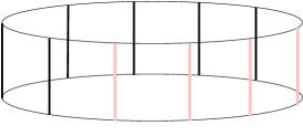
FIG. 1.: A periodically closed cluster of ten rungs. $H_{\rm eff}$ to third order connects at maximum four neighbouring rungs by activated bonds (see text). The connected rungs are printed in grey.

A close inspection of Eqs. (13) and (10) and Tab. I shows that $H_{\rm eff}$ connects a maximum of $l+1$ rungs on a finite cluster of $N$ rungs in $l^{\rm th}$ order. In other words: A maximum of $l$ bonds between neighbouring rungs can be activated in $l^{\rm th}$ order. A bond $\nu$ is said to be activated, if a part of $H_{\rm eff}$, i.e., the specific local operator ${\mathcal{T}}_{n}(\nu)$ in $T_{n}=\sum_{\nu}{\mathcal{T}}_{n}(\nu)$ of $H_{\rm eff}$ (see Eq. (10)), has acted on the two rungs connected by $\nu$.

The linked cluster theorem states that only those processes induced by the $T(\underline{m})$ of $H_{\rm eff}$ contribute to the ground state energy (and all other extensive quantities), in which all activated bonds are linked. Processes involving disconnected active-bond distributions cannot contribute.

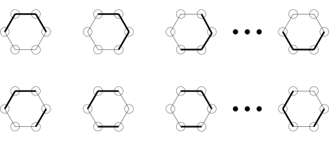
FIG. 2.: A closed ladder-segment of six rungs. Rungs are depicted by circles and (active) bonds between rungs by (thick) solid lines. In a process of order $l=3$ a maximum of 3 bonds can be active. On a closed cluster of $N=6$ there are 6 possibilities to arrange linked bonds (top row). One clearly sees that this number grows linearly in $N$. The given example of 3 disconnected active bonds (bottom row) has 12 possibilities, which would lead to a super-extensive contribution $\propto N^{2}$ to the extensive quantity under study. Thus they do not contribute.

The basic argument is sketched in Fig. 2. This means in our case, that a cluster of $l+1$ rungs is sufficient to calculate the $l^{\rm th}$ order contribution avoiding wrap-arounds as indicated in Fig. 3.

Minimum number of rungs to calculate (16)

the $$l^{\rm th} \epsilon_{0}$$ order contribution to in the (17)

thermodynamic limit (18)

$$=l+1\ .$$ (19)

Once the minimum cluster is specified it is straight forward to calculate $\epsilon_{0}$. The action of $H_{\rm eff}$ on $|0\rangle$, which we have calculated up to 14^th order, on a closed cluster containing 15 rungs is implemented on a computer. Details of this procedure can be found in Ref. [7]. Since $H_{\rm eff}$ conserves the number of triplons we have $H_{\rm eff}|0\rangle\sim|0\rangle$. The constant of proportionality is the ground state energy $E_{0}$ of the 15-rung cluster. The ground state energy per spin is finally given by $\epsilon_{0}=E_{0}/30$. The result is a 14^th order polynomial in $x$. It is the exact energy of the infinite system to the given order

$$\epsilon_{0} =-\frac{3}{8}-\frac{3}{16}{x}^{2}-{\frac{3}{32}}\,{x}^{3}+{\frac{3}{256}}\,{x}^{4}+{\frac{45}{512}}\,{x}^{5}+{\frac{159}{2048}}\,{x}^{6}$$ (20)

$$-{\frac{879}{32768}}\,{x}^{7}-{\frac{4527}{32768}}\,{x}^{8}-{\frac{248391}{2097152}}\,{x}^{9}+{\frac{336527}{4194304}}\,{x}^{10}$$ (21)

$$+\!{\frac{117840599}{402653184}}\,{x}^{11}\!+{\frac{175130171}{805306368}}\,{x}^{12}\!-{\frac{58290422737}{231928233984}}\,{x}^{13}$$ (22)

$$-{\frac{246296576249}{347892350976}}\,{x}^{14}\ .$$ (23)

The coefficients are fractions of integers and therefore free from rounding errors. Our findings agree with the numerical results given by Zheng et al. [32].

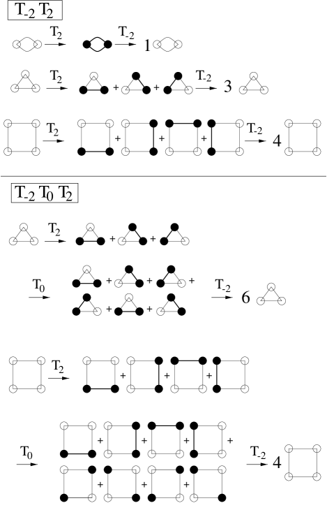
FIG. 3.: Symbols as in Fig. 2; here: rung-singlets (-triplons) are denoted by open (filled) circles. In second order only $T_{-2}T_{2}$ and in third order only $T_{-2}T_{0}T_{2}$ contribute to $\epsilon_{0}$. The action of these operators on the ground state (always to the left) is shown step by step. The upper part shows that in second order the ground state energy per site becomes independent of the cluster-size, if the cluster contains more than two rungs. The lower part shows that wrap-arounds are possible, if the cluster is too small: For the third order contribution to $\epsilon_{0}$ a cluster containing three rungs is undersized. The $T_{0}$ operator in the middle of the process can break up one triplon-pair by moving one of the triplons away by one rung. On the three-rung cluster it joins back the remaining triplon from the other side (wrap-around), which would not be possible in the thermodynamic limit. This process can be avoided by adding one extra rung as buffer, as depicted in the bottom process. Note that $T_{-2}$ destroys two triplons only if they are neighbours. Thus states with diagonally arranged triplons do not contribute. Remembering that one always ends with the ground state $|0\rangle$ if one starts from $|0\rangle$ ($H_{\rm eff}$ conserves the number of triplons!), it is clear that this argument works for all possible processes $T(\underline{m})$ in $H_{\rm eff}$.

The polynomial (23) is depicted as dashed line in Fig. 4. The solid lines correspond to four different Dlog-Padé approximants [55] of this quantity and constitute a reliable extrapolation. The plain series result can be trusted up to $x\approx 0.7$.

FIG. 4.: Ground state energy per spin as function of $x$. The plain series result (23) is depicted as dashed line. Four different Dlog-Padé approximants ([7,6], [8,5], [5,8] and [6,7]) are shown as solid lines.

Since each rung can be in four different states ($s,t^{1},t^{0},t^{-1}$) the Hilbert space has dimension $4^{15}=2^{30}$. Thus the computer calculations used about 1 GByte. They took about 20h. The polynomial will be made available on our home pages [50].

B One-Triplon Dispersion: $H_{1}$

We define $|i\rangle$ to denote the eigen state of $H_{\perp}$ with one triplon on rung $i$ and singlets on all other rungs. The magnetic quantum number $m$ of the triplon at rung $i$ is of no importance in the following considerations, since $H_{\rm eff}$ conserves $m$ and the total spin $S$ (cf. Tab. I). Thus it is not denoted explicitly.

Since $H_{\rm eff}(x)$ conserves the number of triplons the action of $H_{\rm eff}(x)$ on the state $|i\rangle$ is a hopping of the triplon. We define the hopping coefficients

$$a^{\rm cl}_{i;j}(x)=\langle i|H_{\rm eff}(x)|j\rangle\ .$$ (24)

The superscript ${\rm cl}$ indicates that the hopping coefficient might depend on the cluster on which it was calculated.

The hopping coefficients $t_{i;j}$ of the irreducible one-particle operator $H_{1}$ read (see Eqs.9 in Ref. [12])

$$t_{i;j}=\langle i|H_{1}|j\rangle=\langle i|H_{\rm eff}-H_{0}|j\rangle=a^{\rm cl}_{i;j}-E_{0}^{\rm cl}\delta_{i,j}\ .$$ (25)

Since $H_{1}$ is a cluster additive, i.e., an extensive, operator, the coefficients $t_{i;j}$ can be calculated for the infinite system on finite clusters up to some finite order. This is the reason why we dropped the superscript cl from $t_{i;j}$. The cluster ground state energy $E_{0}^{\rm cl}$ must be calculated on the same cluster as the “raw” hopping coefficients $a^{\rm cl}_{i;j}$.

For each order of the coefficient $t_{i;j}$ there exists a minimum cluster which must contain the two rungs $i$ and $j$. To classify the size of the minimum cluster we study how far the triplon motion extends in a given order $l$. Only processes, which take place on linked clusters of active bonds (see previous section), contribute to the extensive thermodynamic hopping coefficients $t_{i;j}$. The minimum cluster must be a linked cluster, which contains the rungs $i$ and $j$.

The action of a single $T_{0}$ operator (first order process) on $|i\rangle$ is to shift the triplon by one as can be readily seen from Tab. I. Somewhat more intricate is the case of the operator $T_{2}$ acting on $|i\rangle$. In any operator-product $T(\underline{m})$ an operator $T_{2}$ is always accompanied by a destruction operator $T_{-2}$. The operator $T_{2}$ creates two triplons on neighbouring sites (triplon-pair) if both of them are occupied by singlets. Suppose that $T_{2}$ is immediately followed by the $T_{-2}$ operator. Then there can be a hopping of the initial triplon by two rungs, if the triplon-pair was created in the immediate vicinity of the triplon at site $i$ to produce a three-triplon state. The situation is depicted in Fig. 5a. This is a second order process. It moves the triplon by two rungs. We could go on like this ($\ldots T_{-2}T_{2}T_{-2}T_{2}$) or we could start to build up a linked chain by iterative application of $T_{2}$ operators, say, to the right of the triplon at site $i$ and then destroy the chain from the left (e.g. $T_{-2}T_{-2}T_{2}T_{2}$). All these processes lead to a maximum motion of the initial triplon by $l$ rungs in $l^{\rm th}$ order.

FIG. 5.: Processes of $H_{\rm eff}$ that lead to a motion of the initial triplon on rung $i$. Active bonds are depicted by thick lines. All processes that contribute to thermodynamic extensive hopping coefficients take place on linked clusters of active bonds. Part a) shows a second order process moving the initial triplon by two rungs. Part b) is a process of order $n+2$ moving the triplon by $n+2$ rungs.

The creation of a triplon-pair not connected to the initial triplon on site $i$ does not lead to any motion of the latter unless there is a sufficient number of $T_{0}$ operators moving the triplon at site $i$ towards the isolated triplon-pair until they form a state with three adjacent triplons as depicted in Fig. 5b. This also leads to a maximum motion of the initial triplon by $l$ rungs in $l^{\rm th}$ order.

All possible combinations of the $T_{2}$, $T_{0}$ and $T_{-2}$ operators that can appear in a $T(\underline{m})$-product of $H_{\rm eff}$ can now be viewed as a product of the processes discussed. So we conclude

maximum motion of one triplon under the action (26)

$$\mbox{of }H_{\rm eff}\mbox{ in }l^{\rm th}\mbox{ order}=l\mbox{ sites .}$$ (27)

Therefore, the minimum cluster to calculate the hopping coefficient $t_{i;j}$ in order $l$ in the thermodynamic limit must contain the two rungs $i$ and $j$, which must not be further apart than $l$ rungs. Additionally the minimum cluster must contain all $l$ bonds that can be activated in all processes moving the triplon from rung $i$ to rung $j$. Fig. 6 illustrates the situation for all coefficients that can be calculated in fourth order.

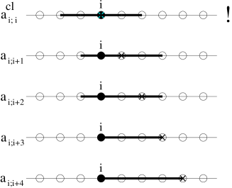
FIG. 6.: All possible hopping coefficients that can be calculated in 4^th order. Again, active bonds are depicted by thick lines. All processes that have to be considered take place on linked clusters. The initial (final) triplon positions are depicted by a filled circle (cross). They are contained in the minimum cluster (cl), which is defined by all active bonds for each coefficient. The exclamation mark next to the $a^{\rm cl}_{i;i}$ cluster is to remind us that we have to subtract the cluster energy $E_{0}^{\rm cl}$ to get the cluster independent hopping coefficient $t_{i;i}=t_{0}$, c.f. Eq. (25)

Because of translational invariance of the original underlying model we can choose a suitable origin on each minimum cluster and it suffices to use a single label for the hopping coefficients, i.e., $t_{i;j}=:t_{i-j}=t_{d}$. Additionally, one has $t_{d}=t_{-d}$ due to inversion symmetry. Note that these relations follow only for the thermodynamic hopping coefficients. In general, the cluster specific coefficients $(t,a)^{\rm cl}$ have lower symmetries. Following the argument above we calculate all thermodynamic hopping coefficients in $14^{\rm th}$ order ($t_{0},t_{1},\ldots t_{14}$) on an open cluster of 15 rungs.

From the thermodynamic cluster-independent hopping coefficients we construct the one-triplon energies. We define the Fourier-transformed states

$$|k\rangle=\frac{1}{\sqrt{N}}\sum_{j}e^{-ikj}|j\rangle\ ,$$ (28)

where $j$ counts the rungs and $N$ is the total number of rungs. Calculating the action of $H_{1}$ on these states yields

$$H_{1}|k\rangle = \frac{1}{\sqrt{N}}\sum_{j,d=-l_{\rm max}}^{l_{\rm max}}e^{-ikj}t_{d}|j+d\rangle$$ (30)

$$= \frac{1}{\sqrt{N}}\sum_{j,d=-l_{\rm max}}^{l_{\rm max}}e^{-ik(j-d)}t_{d}|j\rangle$$ (31)

$$= \sum_{d=-l_{\rm max}}^{l_{\rm max}}e^{ikd}t_{d}\underbrace{\frac{1}{\sqrt{N}}\sum_{j}e^{-ikj}|j\rangle}_{|k\rangle}\ .$$ (32)

Making use of the inversion symmetry $t_{d}=t_{-d}$ yields the real one-triplon dispersion

$$\omega(k;x)=\langle k|H_{1}(x)|k\rangle=t_{0}+2\sum_{d=1}^{l_{\rm max}}t_{d}\cos(dk)\ ,$$ (33)

where the maximum order $l_{\rm max}$ is 14 in our case.

Again, the hopping coefficients $a_{i;j}$ and the corresponding cluster ground state energy $E_{0}$ and therefore the cluster-independent coefficients $t_{d}$ are calculated by implementing the action of $H_{\rm eff}$ on the states $|i\rangle$ on a computer (details in Ref [7]). For fixed one-triplon momentum $k$ the one-triplon dispersion is a 14^th order polynomial in $x$ with real coefficients. Thereby we retrieve and extend the numerical 13^th order result in Ref. [32].

In Fig. 7 the one-triplon dispersion is displayed for five different $x$-values.

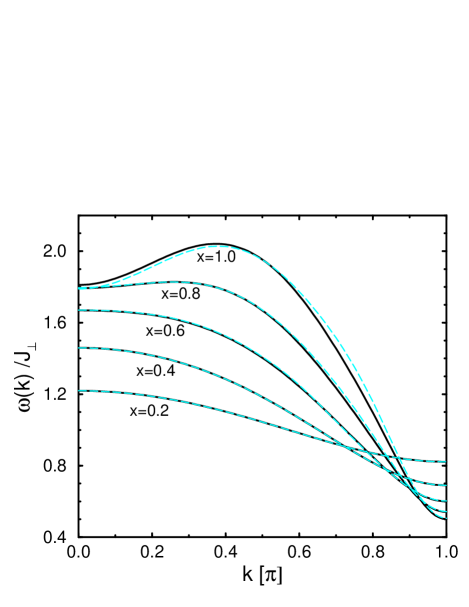
FIG. 7.: One-triplon dispersion for various $x$-values as indicated. The grey dashed lines correspond to plain series results ($x=$0.2, 0.4, 0.6) or to optimized series results ($x=$0.8, 1.0). The solid curves depict our most reliable results obtained by the novel extrapolation scheme explained in Ref. [57].

For $x=$0.2, 0.4 and 0.6 the grey dashed curves represent the results obtained by using the plain series results for the hopping coefficients $t_{d}$. The grey dashed curves for $x=$0.8 and 1.0 result from using the optimized hopping coefficients according to the optimized perturbation theory explained in Sect. V (parameter choice: $\alpha_{\rm opt}=2.9x$). These results are compared to the most reliable extrapolations depicted as solid lines. The latter are obtained by using the novel extrapolation scheme based on a re-expansion of the original series results (polynomials in $x$) in terms of a suitable internal variable $p(x)$ [57].

C Two-Triplon Interaction: $H_{2}$

We define the states $|i,j\rangle$, denoting the eigen state of $H_{\perp}$ with triplon 1 on rung $i$, triplon 2 on rung $j$ and singlets on all other rungs. Two triplons together can form an $S=0$ singlet, an $S=1$ triplet or an $S=2$ quintuplet bound state. Tab. II summarizes these nine states sorted by their total spin $S$ and magnetic quantum number $m$.

By construction $H_{\rm eff}$ conserves the total spin $S$ and the magnetic quantum number $m$. Therefore it is convenient to work in the basis given in Tab. II. This table defines the states $|i,j\rangle^{S,m}$ by the linear combinations in the third column.

m$S$m	$m$
2	2	$|t^{1},t^{1}\rangle$
2	1	$1/\sqrt{2}(|t^{0},t^{1}\rangle+|t^{1},t^{0}\rangle)$
2	0	$1/\sqrt{6}(|t^{-1},t^{1}\rangle+2|t^{0},t^{0}\rangle+|t^{1},t^{-1}\rangle)$
2	-1	$1/\sqrt{2}(|t^{-1},t^{0}\rangle+|t^{0},t^{-1}\rangle)$
2	-2	$|t^{-1},t^{-1}\rangle$
1	1	$1/\sqrt{2}(|t^{1},t^{0}\rangle-|t^{0},t^{1}\rangle)$
1	0	$1/\sqrt{2}(|t^{1},t^{-1}\rangle-|t^{-1},t^{1}\rangle)$
1	-1	$1/\sqrt{2}(|t^{0},t^{-1}\rangle-|t^{-1},t^{0})$
0	0	$1/\sqrt{3}(|t^{0},t^{0}\rangle-|t^{1},t^{-1}\rangle-|t^{-1},t^{1}\rangle)$

TABLE II.: The nine states two triplons can form, combined to states with given quantum numbers $S$ and $m$.

Again, due to triplon conservation the action of $H_{\rm eff}$ on the state $|i,j\rangle$ is to shift the triplons to rung $i^{\prime}$ and rung $j^{\prime}$ conserving also $S$ and $m$. Nothing else is possible. In analogy to Eq. (24) of the preceding section we define the interaction coefficients

$$a^{S,{\rm cl}}_{ij;kl}(x)=\hskip 2.84526pt^{S}\langle i,j|H_{\rm eff}(x)|k,l\rangle^{S}\ .$$ (34)

The coefficients depend on the total spin $S$ but not on the magnetic quantum number $m$. Hence the $m$-index is dropped here and in the following.

The exchange parity is determined by the total spin $S$

$$|i,j\rangle^{S}=(-1)^{S}|j,i\rangle^{S}\ .$$ (35)

This means that we can restrict the description to those states $|i,j\rangle$ for which $i<j$.

Making use of the above the irreducible two-triplon interaction coefficients $t^{S}_{ij;kl}$ follow from

$$t_{ij;kl}^{S}= \ {}^{S}\!\langle i,j|H_{2}|k,l\rangle^{S}=\ ^{S}\!\langle i,j|H_{\rm eff}-H_{1}-H_{0}|k,l\rangle^{S}$$ (36)

$$= a^{S,{\rm cl}}_{ij;kl}-E_{0}^{\rm cl}\delta_{i,k}\delta_{j;l}$$ (37)

$$- t^{{\rm cl}}_{i;k}\delta_{j,l}-t^{{\rm cl}}_{j;l}\delta_{i,k}-t^{{\rm cl}}_{i;l}\delta_{j,k}(-1)^{S}-t^{{\rm cl}}_{j;k}\delta_{i,l}(-1)^{S}\ .$$ (38)

analogous to Eq. (9) in Ref. [12]. Again, $E_{0}^{\rm cl}$ and the one-triplon hopping coefficients $t_{i;j}^{\rm cl}$ must be calculated on the same cluster as the “raw” two-triplon coefficients $a_{ij;kl}^{\rm cl}$. The cluster hopping coefficients $t^{{\rm cl}}_{j;l}$ are needed only in the intermediate steps of the calculation of the irreducible interaction coefficients.

There will be no $t_{ii;kl}$ or $t_{ij;kk}$ since it is not possible to have two triplons on one rung at the same time. This constraint can be viewed as a hardcore repulsion interaction.

The construction of the minimum cluster needed to calculate the $t_{ij;kl}$ in the thermodynamic limit follows the same line of argumentation as in the one-particle section. Generally, the cluster must be large enough to encompass all possible processes in order $l$. The minimum cluster has to include all linked bonds that can be activated in any possible interaction process of length $l$ which leads to state $|i^{\prime},j^{\prime}\rangle$ if one starts with state $|i,j\rangle$. Obviously the rungs $i$, $j$, $i^{\prime}$ and $j^{\prime}$ must be contained in the minimum cluster and they must be connected by active bonds. Fig. 8 shows some interaction coefficients with fixed initial configuration (adjacent triplons) and their associated minimum clusters in 4^th order. All interaction coefficients of order $l$ can be calculated on a cluster containing $l+1$ rungs.

For particular systems there may be symmetries, e.g., spin rotation invariance, or other particularities, e.g., nearest-neighbour coupling only, which prevent certain processes from generating non-vanishing coefficients. Indeed, we found that the spin ladder with nearest-neighbour coupling in order $l$ induces only interaction coefficients of a range which can be determined by distributing $l$ hops among the two triplons. For instance, in 4^th order the triplon at rung $i$ may hop to rung $i-1$ and the triplon at rung $j$ hops to rung $j+3$. Another possible process might be that the triplon at rung $i$ stays at this rung while the triplon at rung $j$ hops to rung $j+4$ or maybe only to rung $j+3$ and so on. This particularity implies for instance that the process shown in Fig. 8c vanishes for the spin ladder system.

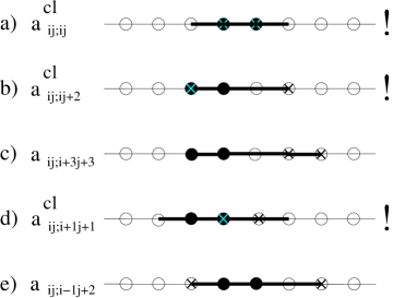
FIG. 8.: Some interaction coefficients that can be calculated in $4^{\rm th}$ order. Initial (final) triplon pairs are denoted by full circles (crosses). The thick solid lines are active bonds between rungs. Exclamation marks indicate that one has to subtract one- or zero-triplon terms according to Eq. (38) to obtain the extensive thermodynamic interaction coefficients.

Due to the translational invariance of the ladder system the momentum $k$ is a good quantum number in the one-triplon sector and the diagonal matrix elements of the Fourier transformed states $|k\rangle$ are the eigen energies $\omega(k)$. With two triplons present only the total momentum $K$ is a good quantum number. The relative momentum $q$ is not conserved and generally leads to the formation of a two-triplon continuum.

To make use of the conserved total momentum we turn to a new basis. As a first step we use center-of-mass coordinates, i.e., $|i,j\rangle^{S}\rightarrow|r,r+d\rangle^{S}=(-1)^{S}|r+d,r\rangle^{S}$, with $r=i$ and $d=j-i$. The restriction $i<j$ (see text below Eq. (35)) translates to $d>0$. We choose a suitable origin, say $k=0$, and rename

$$t_{d;r,d^{\prime}}\equiv\langle r,r+d^{\prime}|H_{2}|0,d\rangle=\langle i,j|H_{2}|k,l\rangle=t_{ij;kl}\ ,$$ (39)

with $d=l$, $r=i$ and $r+d^{\prime}=j$. From Eq. (38) we then obtain

$$t^{S}_{d;r,d^{\prime}} =a^{S,{\rm cl}}_{d;r,d^{\prime}}-E_{0}^{\rm cl}\delta_{0,r}\delta_{d,r+d^{\prime}}-t^{\rm cl}_{r;0}\delta_{d,r+d^{\prime}}-t^{\rm cl}_{d;r+d^{\prime}}\delta_{0,r}$$ (40)

$$-t^{\rm cl}_{0;r+d^{\prime}}\delta_{d,r}(-1)^{S}-t^{\rm cl}_{d;r}\delta_{0,r+d^{\prime}}(-1)^{S}$$ (41)

in the new basis. This is equivalent to the equations emerging from considering the special cases

$$t^{S}_{d;0,d^{\prime}} = a^{S,{\rm cl}}_{d;0,d^{\prime}}-t^{\rm cl}_{d^{\prime}-d}-\delta_{d,d^{\prime}}(t^{\rm cl}_{0}+E^{\rm cl})$$ (43)

$$t^{S}_{d;d-d^{\prime},d^{\prime}} = a^{S,{\rm cl}}_{d;d-d^{\prime},d^{\prime}}-t^{\rm cl}_{d-d^{\prime}}-\delta_{d,d^{\prime}}(t^{\rm cl}_{0}+E^{\rm cl})$$ (44)

$$t^{S}_{d;-d^{\prime},d^{\prime}} = a^{S,{\rm cl}}_{d;-d^{\prime},d^{\prime}}-t^{\rm cl}_{-d-d^{\prime}}(-1)^{S}$$ (45)

$$t^{S}_{d;d,d^{\prime}} = a^{S,{\rm cl}}_{d;d,d^{\prime}}-t^{\rm cl}_{d+d^{\prime}}(-1)^{S}\ .$$ (46)

Otherwise the interaction coefficients $t^{S}_{d;r,d^{\prime}}$ and $a^{S}_{d;r,d^{\prime}}$ are identical.

As a second step the states $|r,r+d\rangle^{S}$ are Fourier transformed with respect to the center-of-mass variable $(r+d/2)$

$$|K,d\rangle^{S} :=\ \ \ \ \ \ \ \frac{1}{\sqrt{N}}\sum_{r}e^{iK(r+d/2)}|r,r+d\rangle^{S}$$ (47)

$$=(-1)^{S}\frac{1}{\sqrt{N}}\sum_{r}e^{iK(r+d/2)}|r+d,r\rangle^{S}$$ (48)

$$\!\!\!\!\!\overset{r\rightarrow r+d}{=}(-1)^{S}\frac{1}{\sqrt{N}}\sum_{r}e^{iK(r-d/2)}|r,r-d\rangle^{S}$$ (49)

$$=(-1)^{S}|K,-d\rangle^{S}\ ,$$ (50)

where $K$ is the conserved total momentum in the Brillouin zone and $N$ is the number of rungs. For fixed $K$ and $S$ the relative distance $d>0$ between two triplons is the only remaining quantum number one has to keep track of.

To obtain the complete two-triplon excitation energies we have to calculate the action of

$$H_{\rm eff}-H_{0}=H_{1}+H_{2}\$$ (51)

on the two-triplon states $|K,d\rangle$. The two addends on the right hand site are considered separately in the following.

The operator $H_{1}$ can move one of the two triplons at maximum. A short calculation yields

$$H_{1}|K,d\rangle^{S}=$$ (52)

$$\frac{1}{\sqrt{N}}\sum_{r}e^{iK(r+d/2)}\!\!\!\!\sum_{n=-l_{\rm max}\atop n\not=d}^{l_{\rm max}}\!\!\!t_{n}(|r+n,r+d\rangle^{S}+|r,r+d-n\rangle^{S})$$ (53)

$$=\sum_{n=-l_{\rm max}\atop n\not=d}^{l_{\rm max}}t_{n}(e^{iKn/2}+e^{-iKn/2})\times$$ (54)

$$\ \ \ \ \times\underbrace{\frac{1}{\sqrt{N}}\sum_{r}e^{iK(r+(d-n)/2)}|r,r+d-n\rangle^{S}}_{|K,d-n\rangle}$$ (55)

$$=2\sum_{n=-l_{\rm max}\atop n\not=d}^{l_{\rm max}}t_{n}\cos\left(K\frac{n}{2}\right)\left[{\rm sgn}(d-n)\right]^{S}|K,|d-n|\rangle^{S}\ .$$ (56)

Here we used the previously calculated matrix-elements $t_{n}=t_{-n}$ (inversion symmetry), which have been calculated to $l_{\rm max}=14$ (cf. preceding subsection). Since we restricted $d>0$ the sgn-function enters the result by Eq. (50). For fixed $K$, $H_{1}$ now appears as a semi-infinite band matrix in the remaining quantum number $d$. Independent of the size of the initial distance $d>0$ between the two triplons, $H_{1}$ will produce states where the distances between the triplons are incremented or decremented by 14 rungs ($l_{\rm max}=14$) at maximum. If the initial distance $d$ is larger than 14, $H_{1}$ continues to produce the same matrix elements on and on for all $d>14$, i.e., the matrix representing $H_{1}$ in the chosen basis for fixed $K$ is semi-infinite with a repeated pattern in the tail. The head of $H_{1}$, i.e., the 14$\times$14 block between states with $d\leq 14$, contains matrix elements with a somewhat more complicated structure. Here the matrix element between the starting distance $d$ and the final distance $d^{\prime}$ is a sum of the direct process $d\rightarrow d^{\prime}$, where one of the triplons has hopped $n$ rungs to the right ($n>0$) or to the left ($n<0$) with $d-n=d^{\prime}>0$, and the indirect process with $d-n=-d^{\prime}<0$. The situation is sketched in Fig. 9. The matrix $H_{1}$ comprises the full thermodynamic one-triplon dynamics in the two-triplon sector for the given order $l_{\rm max}=14$.

The situation is more complex for $H_{2}$. In a first step we find

$$H_{2}|K,d\rangle^{S}=$$ (57)

$$\frac{1}{\sqrt{N}}\sum_{r}e^{iK(r+d/2)}\!\!\!\!\!\!\!\!\sum_{\max\{n+d^{\prime},d-n\}\atop\leq l_{\rm max}}\!\!\!\!\!\!\!\!t_{d;n,d^{\prime}}|r+n,r+n+d^{\prime}\rangle^{S}=$$ (58)

$$\!\!\!\!\!\!\!\!\sum_{\max\{n+d^{\prime},d-n\}\atop\leq l_{\rm max}}\!\!\!\!\!\!\!\!t_{d;n,d^{\prime}}e^{iK(-n+(d-d^{\prime})/2)}|K,d^{\prime}\rangle^{S}\ ,$$ (59)

with the two integers $n\in{\mathbb{Z}}$ and $d^{\prime}\in{\mathbb{N}}$ as summation indices. The positive distances $d$ and $d^{\prime}$ must be smaller or equal to $l_{\rm max}$, since a maximum of $l_{\rm max}$ linked bonds can be produced in this order and all four triplons sites (the two initial sites and the two final sites) must be contained in the resulting linked cluster. The $t_{d;n,d^{\prime}}$ are the matrix elements of $H_{2}$ defined in Eq. (41). The last equality follows from substituting the summation-index $r\rightarrow r+n$.

To simplify the expression further inversion symmetry is used. We have

$$t_{d;r^{\prime},d^{\prime}}=\langle r^{\prime\prime},r^{\prime\prime}+d^{\prime}|H_{2}|r,r+d\rangle\ ,$$ (60)

with $r^{\prime}=r^{\prime\prime}-r$. The thermodynamic interaction coefficient $t_{d;r^{\prime},d^{\prime}}$ is associated with a fixed constellation of initial and final triplon pairs. We define a configuration CON by the set of four positions given by these two pairs ${\rm CON}=\{r,r+d,r^{\prime\prime},r^{\prime\prime}+d^{\prime}\}$. Let $s$ denote the middle of this configuration $s=(\max({\rm CON})-\min({\rm CON}))/2$. Reflecting a configuration about $s$ and interchanging the triplon positions in both initial and final triplon pairs gives

$$t_{d;r^{\prime},d^{\prime}} =\langle r^{\prime\prime},r^{\prime\prime}+d^{\prime}|H_{2}|r,r+d\rangle$$ (61)

$$= \langle 2s-r^{\prime\prime}-d^{\prime},2s-r^{\prime\prime}|H_{2}|2s-r-d,2s-r\rangle$$ (62)

$$=t_{d;d-d^{\prime}-r^{\prime},d^{\prime}}\ .$$ (63)

Possible minus signs cancel since they appear twice. We can now split the sum over $n$ in Eq. (59) in three parts, $n>(d-d^{\prime})/2$, $n<(d-d^{\prime})/2$ and $n=(d-d^{\prime})/2$. The second sum is indexed back to $n>(d-d^{\prime})/2$ by making use of $\sum_{n<j}a_{n}=\sum_{n>j}a_{2j-n}$ where $j:=(d-d^{\prime})/2$

$$H_{2}|K,d\rangle^{S} =\sum_{\max\{n+d^{\prime},d-n\}\leq l_{\rm max}\atop n>(d-d^{\prime})/2\in{\mathbb{Z}}}\left[t_{d;n,d^{\prime}}e^{iK(-n+(d-d^{\prime})/2)}|K,d^{\prime}\rangle^{S}\right.$$ (64)

$$\hskip 28.45274pt\left.+t_{d;d-d^{\prime}-n,d^{\prime}}e^{iK(n-(d-d^{\prime})/2)}|K,d^{\prime}\rangle^{S}\right]$$ (65)

$$\hskip 11.38109pt+\sum_{\max\{n+d^{\prime},d-n\}\leq l_{\rm max}\atop n=(d-d^{\prime})/2\in{\mathbb{Z}}}t_{d;(d-d^{\prime})/2,d^{\prime}}|K,d^{\prime}\rangle^{S}$$ (66)

$$=2\sum_{\max\{n+d^{\prime},d-n\}\leq l_{\rm max}\atop n>(d-d^{\prime})/2\in{\mathbb{Z}}}t_{d;n,d^{\prime}}\cos[K(n-(d-d^{\prime})/2)]|K,d^{\prime}\rangle^{S}$$ (67)

$$\hskip 11.38109pt+\sum_{\max\{n+d^{\prime},d-n\}\leq l_{\rm max}\atop n=(d-d^{\prime})/2\in{\mathbb{Z}}}t_{d;(d-d^{\prime})/2,d^{\prime}}|K,d^{\prime}\rangle^{S}\ .$$ (68)

In contrast to $H_{1}$ the matrix representing $H_{2}$ is of finite dimension due to the finite range of the contributing processes (finite maximum order) expressed by the restrictions of the sums appearing in Eq. (68). In our case the $t_{d;r,d^{\prime}}$ have been calculated up to $l_{\rm max}=13$ giving rise to a $13\times 13$ matrix in the distance $d$ for fixed $K$. Fig. 9 sketches the situation.

Finally, the sum of the two matrixes $H_{1}$ and $H_{2}$ with respect to basis (50) comprises the complete two-triplon dynamics.

The above approach is well justified. At large distances the two-triplon dynamics is governed by independent one-triplon hopping. At smaller distances an additional two-particle interaction occurs given by $t_{d;r,d^{\prime}}$ connecting the state $|r,r+d^{\prime}\rangle$ with state $|0,d\rangle$. The sum $H_{1}+H_{2}$ gives the combined effect of one-triplon hopping and two-triplon interaction. Fig. 10 shows that the interaction coefficients $\langle K,d|H_{2}|K,d\rangle$ for the ladder system indeed drop off rapidly for larger distances.

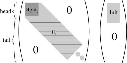
FIG. 9.: The left part of the figure schematically shows the matrix representation of $H_{1}$ and $H_{2}$ in the two-triplon $\{|K,d\rangle\}$ basis (50). The matrix $H_{1}$ has elements in the whole grey area, while $H_{2}$ has elements in the dark grey area only. We calculated the elements of $H_{2}$ up to order 13 and those of $H_{1}$ up to order 14, so that $H_{2}$ is a finite $13\times 13$ matrix and $H_{1}$ a semi-infinite band matrix, whose width is 28, see Eqs. (56) and (68) for further information. The sum of $H_{1}$ and $H_{2}$ represents $H_{\rm eff}$ in the two-triplon sector to the given orders. The right part shows the initial vector $|\text{Init}\rangle={\mathcal{O}}_{\rm eff}|0\rangle$ as calculated in Sect. III for the two-triplon sector. Since we calculated ${\mathcal{O}}_{\rm eff}$ up to order 10, $|\text{Init}\rangle$ is a vector of dimension 10 in the $\{|K,d\rangle\}$ basis. The Green function ${\mathcal{G}}$ (Eq. (4)) is calculated by tridiagonalization, more information in Sect. IV. For $K$ and $x$ fixed, the elements of the matrix and the vector reduce to real numbers.

FIG. 10.: Expectation values of some diagonal elements of $H_{2}$ (pure two-triplon interaction) for the ladder system in the $\{|K,d\rangle\}$ basis for various $K$-values and $x$ set to 0.6 as function of the remaining quantum number $d$. Clearly, the irreducible two-triplon interaction coefficients drop off rapidly with increasing relative distance $d$ between the two triplons. Non-diagonal elements behave in a similar fashion. At larger distances two triplons are asymptotically free.

Taking the perturbation expansion up to order $l_{\rm max}$ allows to calculate the irreducible two-particle interaction up to a distance $l$ between the two particles correctly within order $l_{\rm max}$. No processes involving larger distances appear. But the part of the two-particle sector that can be described by one-particle dynamics alone is taken into account for all distances between the two particles and describes hopping processes of range $\leq l_{\rm max}$ correctly within order $l_{\rm max}$.

At $K=\pi$, the smallest eigen value of $\tilde{H_{1}}+H_{2}$, where $\tilde{H_{1}}$ is the upper left $13\times 13$ sub-matrix of $H_{1}$, can be extracted as a 13^th order polynomial in $x$ and identified as the (lowest) bound state. This is possible because at $K=\pi$, the relative motion of the two triplons is of order $x^{2}$ while the interaction enters in order $x$. Hence the interaction dominates over the kinetics for $x\to 0$ so that a local bound pair is the simple eigen state for vanishing $x$. Our results extend the results by Zheng et al. [11] for $S=1$ from 12^th to 13^th order, and for $S=0$ from 7^th to 13^th order. The polynomials will be made available on our web pages [50].

III Transformation of the observables

A General Aspects

The continuous unitary transformation of observables has been explained in detail in Ref. [12]. Here we briefly review the most important general aspects before we describe the procedure for the spin ladder in detail.

Using the same transformation as for the Hamiltonian we derive a series expansion (similar to Eq. (13)) for the effective observable ${\mathcal{O}}_{\rm eff}$ onto which a given initial observable ${\mathcal{O}}$ is mapped by the perturbative CUT procedure

$${\mathcal{O}_{\rm eff}}(x)=\sum_{k=0}^{\infty}x^{k}\sum_{i=1}^{k+1}\sum_{|\underline{m}|=k}\tilde{C}(\underline{m};i){\mathcal{O}}(\underline{m};i)\ ,$$ (69)

where

$${\mathcal{O}}(\underline{m};i):=T_{m_{1}}\cdots T_{m_{i-1}}{\mathcal{O}}T_{m_{i}}\cdots T_{m_{k}}\ .$$ (70)

The operators $T_{i}$ are the same as in the Hamilton transformation. The coefficients $\tilde{C}(\underline{m};i)$ can again be calculated on a computer. They are fractions of integers [12].

The effective observables are described by weighted virtual excitation processes $T(\underline{m})$ interrupted by processes induced by the observable as given in Eq. (70). Sometimes it is convenient to seek for a decomposition of ${\mathcal{O}}$ with respect to its action on the number of particles

$${\mathcal{O}}=\sum_{n=-N}^{N}T^{\prime}_{n}\ ,$$ (71)

where $T^{\prime}_{n}$ creates $n$ particles or destroys them if $n<0$.

An important point is that ${\mathcal{O}}_{\rm eff}$ is not an energy quanta conserving quantity, i.e., it does not conserve the number of triplons in the spin ladder system. This is formally expressed by the fact that the sum over $\underline{m}$ is not restricted to $M(\underline{m})=0$, so that ${\mathcal{O}}_{\rm eff}$ can add or subtract an arbitrary number of particles.

The effective operators ${\mathcal{O}}_{\rm eff}$ can be decomposed in a sum of cluster-additive operators ${\mathcal{O}}_{p,n}$, for which the linked cluster theorem can be used

$${\mathcal{O}}_{\rm eff}=\sum_{n=0}^{\infty}\sum_{p\geq-n}{\mathcal{O}}_{p,n}\ .$$ (72)

Here $p$ indicates how many particles are created ($p\geq 0$) or destroyed ($p<0$) by ${\mathcal{O}}_{p,n}$. The subindex $n\geq 0$ indicates the minimum number of particles that must be present for ${\mathcal{O}}_{p,n}$ to have a non zero action. The action of the operator ${\mathcal{O}}_{p,n}$ on a state containing less than $n$ particles is zero. Further definitions and details concerning the operators ${\mathcal{O}}_{p,n}$ can be found in Ref. [12].

Focusing on $T=0$ experiments in the following, we treat only the operators ${\mathcal{O}}_{p\geq 0,0}$. Their interpretation is particularly simple. The effective observable ${\mathcal{O}}_{\rm eff}$ acting on the $T=0$ state, i.e., the ground state or excitation vacuum, respectively, decomposes in a sum of the operators ${\mathcal{O}}_{p\geq 0,0}$, each injecting $p=0,1,2\ldots$ triplons into the system. In Ref. [12] we showed that the ${\mathcal{O}}_{p\geq 0,0}$ can be directly calculated from the action of ${\mathcal{O}}_{\rm eff}$ on $|0\rangle$ on minimum finite clusters. No extra terms have to be subtracted to obtain thermodynamic results. The calculations can again be implemented on a computer in analogy to what was done for the Hamiltonian.

To be more specific let ${\mathcal{O}}$ be a locally acting observable injecting triplons at a specific site $r$ of the ladder. Then the effective observable reads

$${\mathcal{O}}_{\rm eff}(r)|0\rangle=\sum_{p\geq 0}{\mathcal{O}}_{p,0}(r)|0\rangle$$ (73)

$$=c|0\rangle+\sum_{n=-l_{\rm max}}^{l_{\rm max}}c_{n}|r+n\rangle+$$ (74)

$$\hskip 8.53581pt+\sum_{n,n^{\prime}\atop|n|+|n^{\prime}|\leq l_{\rm max}}c_{n,n^{\prime}}|r+n,r+n^{\prime}\rangle+\cdots\ .$$ (75)

The restriction $|n|+|n^{\prime}|\leq l_{\rm max}$ for the third sum reflects the fact that the two triplons, after being injected, cannot undergo more rung-to-rung hops in total than the maximum order $l_{\rm max}$. Therefore, the maximum distance $p=|n-n^{\prime}|$ occurring is $l$ in order $l$ for the spin ladder system.

Once the coefficients $c$ are calculated the spectral weights $I_{N}$ are accessible, which are contained in the different particle-sectors characterized by the number ${N}$ of particles injected

$$I_{N} =\langle 0|{\mathcal{O}}_{-N,0}(r){\mathcal{O}}_{N,0}(r)|0\rangle$$ (76)

$$=\sum_{n_{1},\ldots,n_{N}}|\langle r+n_{1},\ldots,r+n_{N}|{\mathcal{O}}_{N,0}(r)|0\rangle|^{2}$$ (77)

$$=\sum_{n_{1},\ldots,n_{N}}|c_{n_{1},\ldots,n_{N}}|^{2}\ .$$ (78)

If the total weight $I_{\rm tot}$ of the operator is also known, for instance via the sum rule $I_{\rm tot}=\langle 0|{\mathcal{O}}^{2}|0\rangle-\langle 0|{\mathcal{O}}|0\rangle^{2}$, the relative weights of the individual particle sectors $I_{N}/I_{\rm tot}$ can be calculated. They serve as an important criterion to judge the applicability of our approach. If most of the weight can be found in sectors of low quasi-particle number and sectors of higher particle number can be safely neglected the approach will work fine. The chosen particles constitute a suitable basis to describe the system. This argument has been used by Schmidt and Uhrig [18] to show, that the triplon is a well suited particle to describe the one- dimensional spin chain. There basically all the spectral weight is captured by one and two triplons.

So far local observables ${\mathcal{O}}(r)$ were considered. A real experiment, however, couples to the system in a global fashion. Due to translational invariance the injected particles (here triplons) have a total momentum $K$. Thus we define the global observables in momentum space representations

$${\mathcal{O}}_{\rm eff}(K)|0\rangle =\sum_{p\geq 0}{\mathcal{O}}_{p,n}(K)|0\rangle$$ (79)

$$=\sum_{p\geq 0}\frac{1}{\sqrt{N}}\sum_{r=1}^{N}e^{iKr}{\mathcal{O}}_{p,0}(r)|0\rangle\ ,$$ (80)

where $N$ is the number of rungs in the system. Let us investigate the one- and two-triplon sectors separately. In the one-triplon sector we have (here $K$ is the one-triplon momentum $k$)

$${\mathcal{O}}_{1,0}(k)|0\rangle =\frac{1}{\sqrt{N}}\sum_{r}e^{ikr}\sum_{n}c_{n}|r+n\rangle$$ (81)

$$=\sum_{n}c_{n}e^{-ikn}\frac{1}{\sqrt{N}}\sum_{r}e^{ikr}|r\rangle$$ (82)

$$=\sum_{n}c_{n}e^{-ikn}|k\rangle\ .$$ (83)

We used the same definition for $|k\rangle$ as introduced in Sect. II. Due to inversion symmetry $c_{n}=c_{-n}$ holds. Thus Eq. (83) simplifies to

$$\langle k|{\mathcal{O}}_{1,0}(k)|0\rangle =A_{k}=c_{0}+2\sum_{n}c_{n}\cos(kn)\ .$$ (84)

Somewhat more complex is the two-triplon sector

$${\mathcal{O}}_{2,0}(K)|0\rangle=\frac{1}{\sqrt{N}}\sum_{r=1}^{N}e^{iKr}\sum_{n,n^{\prime}}c_{n,n^{\prime}}|r+n,r+n^{\prime}\rangle$$ (85)

$$=\sum_{n,d}c_{n,n+d}e^{-iK(n+d/2)}\frac{1}{\sqrt{N}}\sum_{r}e^{iK(r+d/2)}|r,r+d\rangle$$ (86)

$$=\sum_{n,d}c_{n,n+d}e^{-iK(n+d/2)}|K,d\rangle$$ (87)

$$=\sum_{d}A_{K,d}|K,d\rangle\ ,$$ (88)

where we defined the relative distance $d=n^{\prime}-n$ between the two injected triplons. The definition of $|K,d\rangle$ is taken from Sect. II. Again, inversion symmetry, here $c_{n,n^{\prime}}=(-1)^{S}c_{-n,-n^{\prime}}$, can be used to obtain real results for the coefficients $A_{K,d}$. The variable $S\in\{0,1,2\}$, which is a good quantum number, denotes the total spin of the injected triplon pair.

The action of ${\mathcal{O}}_{\rm eff}$ from the ground state into the two-triplon space produces the states $|K,d\rangle$ with $0<d\leq l_{\rm max}$ in order $l_{\rm max}$. Thus, for fixed $K$, the action of ${\mathcal{O}}_{\rm eff}$ may be visualized as a vector in the remaining quantum number $d$ of which the first $l_{\rm max}$ entries are the $A_{K,d}$ of Eq. (88). All other entries are zero. This vector, labeled initial vector $|\text{Init}\rangle$ for reasons given in Sect. IV, is depicted in Fig. 9 together with the matrix representing $H_{\rm eff}$ for fixed $K$ in the two-triplon sector.

B Observables in the Spin Ladder

We now turn to the evaluation of the observables of interest in the ladder system. We calculated the $\tilde{C}(\underline{m};i)$ in Eq. (69) up to and including order $l_{\rm max}=10$ for the problem under study. The four local operators considered are

$${\mathcal{O}}^{\rm I}(r) = {\mathbf{S}}_{1,r}{\mathbf{S}}_{2,r}={\mathcal{T}}^{\rm I}_{0}$$ (90)

$${\mathcal{O}}^{\rm II}_{l}(r) = {\mathbf{S}}_{l,r}{\mathbf{S}}_{l,r+1}$$ (91)

$$= \frac{1}{4}\left({\mathcal{T}}_{-2}+{\mathcal{T}}_{0}+{\mathcal{T}}_{2}+{\mathcal{T}}^{\rm II}_{-1}+{\mathcal{T}}^{\rm II}_{1}\right)$$ (92)

$${\mathcal{O}}^{\rm III}(r) = {\mathbf{S}}^{z}_{1,r}-{\mathbf{S}}^{z}_{2,r}={\mathcal{T}}^{\rm III}_{-1}+{\mathcal{T}}^{\rm III}_{1}$$ (93)

$${\mathcal{O}}^{\rm IV}(r) = {\mathbf{S}}^{z}_{1,r}+{\mathbf{S}}^{z}_{2,r}={\mathcal{T}}^{\rm IV}_{0}\ ,$$ (94)

where the decompositions are either given in Table I for the ${\mathcal{T}}$ or in Table II for the ${\mathcal{T}}^{\mu}$, with $\mu\in\{{\rm I,II,III,IV}\}$. The index $l=1,2$ in Eq. (91) denotes the leg on which the observable operates.

	$4{\mathcal{T}}^{\rm I}_{0}$
$|s\rangle$	$\longrightarrow$	$-3|s\rangle$
$|t^{i}\rangle$	$\longrightarrow$	$|t^{i}\rangle$
	$4{\mathcal{T}}^{\rm II}_{1}$
$|s,t^{1}\rangle$	$\longrightarrow$	$|t^{1},t^{0}\rangle-|t^{0},t^{1}\rangle$
$|t^{1},s\rangle$	$\longrightarrow$	$-|t^{1},t^{0}\rangle+|t^{0},t^{1}\rangle$
$|s,t^{0}\rangle$	$\longrightarrow$	$|t^{1},t^{-1}\rangle+|t^{-1},t^{1}\rangle$
$|t^{0},s\rangle$	$\longrightarrow$	$-|t^{1},t^{-1}\rangle+|t^{-1},t^{1}\rangle$
$|s,t^{-1}\rangle$	$\longrightarrow$	$|t^{0},t^{-1}\rangle-|t^{-1},t^{0}\rangle$
$|t^{-1},s\rangle$	$\longrightarrow$	$-|t^{0},t^{-1}\rangle+|t^{-1},t^{0}\rangle$
	${\mathcal{T}}^{\rm III}_{1}$
$|s\rangle$	$\longrightarrow$	$|t^{0}\rangle$
$|t^{\pm 1}\rangle$	$\longrightarrow$	$0$
	${\mathcal{T}}^{\rm IV}_{0}$
$|s\rangle$	$\longrightarrow$	$0$
$|t^{i}\rangle$	$\longrightarrow$	$i|t^{i}\rangle$

TABLE III.: Action of the local operators ${\mathcal{T}}^{\mu}_{i}$ appearing in Eqs. (III B). The notation is the same as in Table I.

We start with a simple symmetry property. Let ${\mathcal{P}}$ denote the operator of reflection about the center-line of the ladder as depicted in Fig. 11.

FIG. 11.: The operator ${\mathcal{P}}$ reflects about the depicted axis. A single rung-singlet (-triplon) has odd (even) parity with respect to ${\mathcal{P}}$. The action of ${\mathcal{P}}$ on the rung-singlet ground state is defined to be of even parity ${\mathcal{P}}|0\rangle=|0\rangle$. If in $|0\rangle$ one singlet is substituted by a triplon we get the state $|1\rangle$ and ${\mathcal{P}}|1\rangle=-|1\rangle$. Generally, one has ${\mathcal{P}}|n\rangle=(-1)^{n}|n\rangle$.

If $|n\rangle$ denotes a state with $n$ rungs excited to triplons while all other rungs are in the singlet state we find ${\mathcal{P}}|n\rangle=(-1)^{n}|n\rangle$, see caption of Fig. 11. The state $|n\rangle$ might be a linear combination of many $n$-triplon states so no generality is lost in writing

$${\mathcal{O}}_{\rm eff}|0\rangle=\sum_{n\geq 0}|n\rangle\ .$$ (95)

The parity of the ladder observables introduced in Eqs. (III B) with respect to ${\mathcal{P}}$ is clear from their definition: ${\mathcal{O}}^{\rm III}$ is odd while ${\mathcal{O}}^{\rm I}$ and ${\mathcal{O}}^{\rm IV}$ are even with respect to ${\mathcal{P}}$, just as the symmetriezed observable ${\mathcal{O}}^{\rm II}=({\mathcal{O}}^{\rm II}_{1}+{\mathcal{O}}^{\rm II}_{2})/2$. These parities are conserved under the CUT so that ${\mathcal{P}}$ applied on both sides of Eq. (95) yields

$${\mathcal{O}}_{\rm eff}|0\rangle=\left\{\begin{array}[]{cc}\sum_{n}|2n\rangle,&{\mathcal{O}}_{\rm eff}\mbox{ even}\\ \sum_{n}|2n+1\rangle,&{\mathcal{O}}_{\rm eff}\mbox{ odd}\end{array}\right.\ .$$ (96)

We thus find that an even (odd) parity of ${\mathcal{O}}_{\rm eff}$ implies that ${\mathcal{O}}_{\rm eff}$ can inject an even (odd) number of triplons into the system.

The coefficients $c$ in Eq. (75) have been calculated for the one- and two-triplon case on a computer in a similar fashion as the coefficients $t$ for the effective Hamiltonian. The implementation of ${\mathcal{O}}_{\rm eff}$ acting on the ground state $|0\rangle$ follows the same line as described in detail for $H_{\rm eff}$ in Ref. [7]. The minimum clusters necessary for some fixed order arise from the same considerations as in Sect. II. Again, the coefficients $c$ are rational numbers which we computed up to $l_{\rm max}=10{{}^{\rm th}}$ order for the observables in Eqs. (III B).

First physically interesting quantities are the spectral weights of the observables. As illustrated in Eq. (78) the spectral weight contained in the $N$-triplon sector, $I_{N}$, is readily given by the coefficients $c$. Under certain circumstances the total weight $I_{\rm tot}=I_{0}+I_{1}+I_{2}+\ldots$ of an observable might be accessible from sum rules. Let us consider the $S=0$ operator ${\mathcal{O}}_{\rm eff}^{\rm II}$ in Eq. (91) as an example. Here the total weight $I_{\rm tot}(x)$ can be obtained from the ground state energy per spin $\epsilon_{0}(x)$ given in Eq. (23). Since $2{\mathcal{O}}_{\rm eff}^{\rm II}(x)=\partial/\partial xH_{\rm eff}(x)$ (cf. Eqs. (1) and (7)) the sum rule can be expressed in terms of the effective Hamiltonian, giving rise to

$$I_{\rm tot} =\sum_{N=0}^{\infty}I_{N}=\langle 0|{\mathcal{O}}^{2}|0\rangle-\langle 0|{\mathcal{O}}|0\rangle^{2}$$ (97)

$$=\frac{3}{16}-\frac{Y}{2}-\frac{Y^{2}}{2}\ ,$$ (98)

with $Y:=\partial\epsilon_{0}/\partial x$. If both, $I_{\rm tot}$ and some of the $I_{N}$ are known, we can calculate the corresponding relative spectral weights $I_{N}/I_{\rm tot}$ as functions of $x$. Fig. 12 shows the resulting relative weights for the observable ${\mathcal{O}}^{\rm II}_{\rm eff}$ for the first four triplon sectors.

FIG. 12.: Relative weights for the S=0 operator $S_{1,i}S_{1,i+1}$ (Eq. (91)). The $I_{\rm N}$ are calculated according to Eq. (78) up to and including order 10, 8 and 7 in $x$ for the $c_{\{n\}}$ for $N=$2, 3 and 4, respectively. The total intensity $I_{\rm tot}$ has been extracted from the 14^th order result for the ground state energy per spin according to Eq. (98). This figure represents an improvement of a similar figures in Ref. [13]. The expansion for $I_{3}$ has been extended by one order and the extrapolation of $I_{2}$ has been improved.

Since one cannot form an $S=0$ object from a single rung-triplon there is no $I_{1}$ for this observable. The contribution of $I_{5}/I_{\rm tot}$ is of order 10^-3 leading to no visible changes in Fig. 12. Contributions of higher triplon channels are expected to be even smaller. All relative weights add up to unity. As can be seen in Fig. 12 the first four relative weights fulfill this requirement with great precision. For $x=0$ the singlet made from two isolated-rung triplons contains the full weight of the considered operator. As $x$ increases the triplons start to polarize their environment, the two-triplon weight decreases and multi-triplon states gain weight. A similar figure for the $S=1$ operator $S_{1,i}^{z}$ can be found in Ref. [13] (Fig. 2).

From the depicted result we conclude that the triplon is an excellent choice for quasi-particle in the ladder system. For $x$ not too large most of the spectral weight is captured by a few triplons. Calculations containing only a few triplons suffice to explain most of the physics for $x\lesssim 1.5$.

Eqs. (84) and (88) show how the momentum depend coefficients $A_{k}$ (one-triplon) and $A_{K,d}$ (two-triplons) can be calculated from the corresponding $c$-coefficients. For the two-triplon sector we provide some examples to 3^rd order in $x$. The shown coefficients $A_{K,d}$ belong to the symmetrized observable ${\mathcal{O}}^{\rm II}=({\mathcal{O}}^{\rm II}_{1}+{\mathcal{O}}^{\rm II}_{2})/2$ or to the observable ${\mathcal{O}}^{\rm IV}$, respectively,

$$A_{K,1}^{\rm II} =-\frac{1}{4}-\frac{1}{8}\,x+\frac{1}{8}\,\left(\frac{5}{8}\,\cos\left(K\right)+\frac{5}{8}\right){x}^{2}$$ (99)

$$+\frac{1}{8}\,\left({\frac{25}{16}}+{\frac{17}{16}}\,\cos\left(K\right)\right){x}^{3}$$ (100)

$$A_{K,2}^{\rm II} =\frac{1}{8}\,\cos\left(\frac{1}{2}\,K\right)x+\frac{1}{16}\,\cos\left(\frac{1}{2}\,K\right){x}^{2}$$ (101)

$$+\frac{1}{16}\,\left(-{\frac{37}{16}}\,\cos\left(\frac{1}{2}\,K\right)-{\frac{13}{16}}\,\cos\left(\frac{3}{2}\,K\right)\right){x}^{3}$$ (102)

$$A_{K,1}^{\rm IV} =\frac{1}{2}\,x\sin\left(\frac{1}{2}\,K\right)+\frac{1}{4}\,{x}^{2}\sin\left(\frac{1}{2}\,K\right)$$ (103)

$$-{\frac{11}{64}}\,{x}^{3}\sin\left(\frac{1}{2}\,K\right)\ .$$ (104)

Fig. 13 displays the coefficients of ${\mathcal{O}}^{II}$ and ${\mathcal{O}}^{IV}$ as function of the relative distance $d$ for fixed $K$-values at $x=1$. The depicted values are obtained by using standard Padé techniques for the $A_{K,d}$ as polynomials in $x$ for fixed momentum $K$.

FIG. 13.: The two-triplon momentum dependent coefficients $A_{K,d}$ of the observables ${\mathcal{O}}^{II}$ and ${\mathcal{O}}^{IV}$ for all calculated distances $d$ at $x=1$ and momenta as indicated. The coefficients rapidly drop to zero with increasing distance. It is not necessary to go to larger orders, i.e., distances.

All calculated one-triplon ($A_{k}$) and two-triplon ($A_{K,d}$) coefficients will be made available on our home pages [50].

IV Evaluating the Green Function

We are now in the position to calculate the zero temperature one- and two-triplon spectral densities associated with the ladder observables introduced in the last section. To this end we start by analyzing the energy and momentum resolved retarded zero temperature Green function

$${\mathcal{G}}^{\mathcal{O}}(K,\omega) =$$ (105)

$$\left\langle\psi_{0}\left|{\mathcal{O}}^{\dagger}(K)\frac{1}{\omega-\left(H(K)-E_{0}\right)+i0^{+}}{\mathcal{O}}(K)\right|\psi_{0}\right\rangle\ ,$$ (106)

from which the spectral density ${\mathcal{S}}(K,w)$ follows by taking the negative imaginary part. As explained in Sect. I.B, all operators can be replaced by their effective counterparts after the transformation and the ground state $|\psi_{0}\rangle$ by the triplon vacuum $|0\rangle$.

A One-Triplon Green Function

In the one-triplon case the calculation is particularly simple. Using Dirac’s identity

$$\frac{1}{x-x_{0}\pm i0^{+}}={\mathcal{P}}\frac{1}{x-x_{0}}\mp i\pi\delta(x-x_{0})\ ,$$ (107)

where ${\mathcal{P}}$ denotes Cauchy’s principal value, we find

$${\mathcal{S}}(k,\omega) =\left\langle 0\left|{\mathcal{O}}^{\dagger}_{1,0}(k)\delta(\omega-H_{1}){\mathcal{O}}_{1,0}^{\phantom{\dagger}}(k)\right|0\right\rangle$$ (108)

$$=|A_{k}|^{2}\left\langle k\left|\delta(w-H_{1})\right|k\right\rangle$$ (109)

$$=|A_{k}|^{2}\delta\left(\omega-\omega(k)\right)\ .$$ (110)

The one-triplon dispersion $\omega(k)$ and the observable coefficient $A_{k}$ are readily given by Eqs. (33) and (84), respectively. At each point $(k,\omega(k))$ the corresponding weight is given by the square of the modulus of $A_{k}$ which is a polynomial in $x$. The result is thus obtained by assigning a $\delta$-function with corresponding weight to each point $(k,\omega(k))$.

B Two-Triplon Green Function

For the two-triplon case we choose to evaluate the effective Green function by tridiagonalization. This leads to the continued fraction expression ([58, 59, 60], for overviews see Refs. [61, 62])

$${\mathcal{G}}_{2,0}^{\mathcal{O}}(K,\omega)=\frac{\langle 0|{\mathcal{O}}^{\dagger}_{2,0}(K){\mathcal{O}}_{2,0}^{\phantom{\dagger}}(K)|0\rangle}{\omega-a_{0}-{\displaystyle\frac{b_{1}^{2}}{\omega-a_{1}-{\displaystyle\frac{b_{2}^{2}}{\omega-\cdots}}}}}\ ,$$ (111)

where we can also write $\sum_{d}|A_{K,d}|^{2}$ for the expression in the numerator on the right hand side. The coefficients $A_{K,d}$ are given by Eq. (88). The coefficients $a_{i}$ and $b_{i}^{2}$ are calculated by repeated application of $H_{\rm eff}-H_{0}=H_{1}+H_{2}$ on the initial two-triplon momentum state $|{\rm Init}\rangle=|f_{0}\rangle={\mathcal{O}}_{2,0}(K)|0\rangle$. The action of $H_{1}$ and $H_{2}$ on these states have been calculated previously. The results are given in Eqs. (56) and (68), respectively.

Setting the state $|f_{-1}\rangle=0$ the recursion (Lanczos tridiagonalization)

$$|f_{n+1}\rangle=(H_{1}+H_{2})|f_{n}\rangle-a_{n}|f_{n}\rangle-b_{n}^{2}|f_{n-1}\rangle\ \ ,\ n\in{\mathbb{N}}$$ (112)

generates a set of orthogonal states $|f_{n}\rangle$ if the coefficients are defined according to

$$a_{n}=\frac{\langle f_{n}|(H_{1}+H_{2})|f_{n}\rangle}{\langle f_{n}|f_{n}\rangle}\ ,\ \ \ \ \ b_{n+1}^{2}=\frac{\langle f_{n+1}|f_{n+1}\rangle}{\langle f_{n}|f_{n}\rangle}\ .$$ (113)

In the generated $\{|f_{n}\rangle\}$-basis $H_{\rm eff}$ is a tridiagonal matrix, where the $a_{i}$ are the diagonal matrix elements and the $b_{i}$ are the elements on the second diagonal. All other matrix elements are zero.

Fig. 9 illustrates the procedure for the two-triplon sector. For fixed $K$ the relative (positive) distance $d$ between the two injected triplons is the only remaining quantum number. In this basis $H_{1}+H_{2}$ is represented as a matrix (left side). The matrix elements are polynomials in the perturbation parameter $x$. We have to apply this matrix iteratively to the $|f_{n}\rangle$. The components $A_{K,d}$ of the initial vector $|f_{0}\rangle=|{\rm Init}\rangle$ are polynomials in $x$ for fixed $K$. By this procedure a new basis $|f_{n}\rangle$ is generated in which the fairly complicated matrix in Fig. 9 is simplified to a tridiagonal one.

The general case of more than two triplons can be treated similarly. For $n$ triplons we have to consider the conserved total momentum $K$ and $n-1$ relative distances. Then, for fixed $K$, $|{\rm Init}\rangle$ and $H_{\rm eff}$ are still represented by a vector and matrices, respectively. But they are more complicated. For three triplons we obviously have to apply $H_{1}+H_{2}+H_{3}$ to $|{\rm Init}\rangle$. For four triplons $H_{4}$ is added and so on. The calculation of $H_{n}$ with $n>2$ is indicated in Ref. [12].

Thus, the full many-particle problem is effectively reduced to a few-particle problem! Further, after fixing the parameter value $x$ the coefficients $a_{i}$ and $b_{i}$ are obtained by the numerical Lanczos tridiagonalization, which is left to the computer. This procedure is realized for fixed $x$ and $K$. For the spin ladder we were able to implement a maximum relative distance $d$ of $\approx 10000$, allowing to repeat the recursion about 650 times giving the first 650 coefficients $a_{i}$ and $b^{2}_{i}$.

Thus the chosen method to evaluate the effective Green function introduces no quantitative finite size effects. The problem of calculating the spectral densities for given effective Hamiltonians and observables comprises the two quantum numbers $K$ and $d$ in the two-triplon sector. For each triplon more, there is one more relative distance to be considered, see above. Our calculations are exact and without finite-size effect to the given order for the total momentum $K$.

There are two approximations that involve the relative distance $d$. They will be discussed in the following. The prevailing approximation is caused by the finiteness of the perturbative calculations. The true many-triplon interactions are accounted for only if all involved particles are within a certain finite distance to each other. This approximation is controlled, since one generically observes a rather sharp drop of the interaction matrix elements with increasing distances (see Fig. 10 for the spin ladder). Gapped systems with finite correlation lengths are well suited to be tackled by our method. Difficulties arise if the correlations drop slowly with increasing distances. In this case the truncations in real-space might not be justified.

A second minor approximation to the results involving the relative distance $d$ is introduced by truncating the continued fraction expansion of the Green function. However, allowing for distances of up to 10000 lattice spacings as in the ladder example guarantees that this error is extremely small in comparison to the error introduced by truncating the perturbative expansion as discussed in the preceding paragraph.

The finiteness of the continued fraction can be partly compensated by suitable terminations as shall be explained in the following subsection.

C Terminator

The spectral density ${\mathcal{S}}(K,\omega)$ at fixed $K$ as obtained from the truncated continued fraction (111) of the effective Green function has poles at the zeros of the denominator. Thus, ${\mathcal{S}}$ would be a collection of sharp peaks. A slight broadening of ${\mathcal{S}}$ via $\omega\rightarrow\omega+i\delta$ ($\delta$ small) in ${\mathcal{G}}$ will smear out all poles to give a continuous function for all practical purposes. However, we can achieve perfect resolution of ${\mathcal{S}}$ as continuous function by introducing a proper termination of the continued fraction exploiting the one-dimensionality of the considered model.

For fixed total momentum $K$ the (upper) lower band edges ($\epsilon_{\rm ub}$) $\epsilon_{\rm lb}$ of the two-triplon continuum can be calculated from the one-triplon dispersion $\omega_{1}$ (33). All energies of the two-triplon continuum are seized by

$$\omega_{2}(K,q)=\omega_{1}\left(K/2+q\right)+\omega_{1}\left(K/2-q\right)\ ,$$ (114)

where $q\in[-\pi,\pi]$ denotes the relative momentum. Therefore, we can calculate $\epsilon_{\rm ub}$ and $\epsilon_{\rm lb}$ from the one-triplon dispersion

$$\epsilon_{\rm ub}(K) =\max_{q}(\omega_{2}(K,q))$$ (115)

$$\epsilon_{\rm lb}(K) =\min_{q}(\omega_{2}(K,q))\ .$$ (116)

For fixed $K$ the upper and lower band edges $\epsilon_{\rm ub}$ and $\epsilon_{\rm lb}$ determine the values to which the continued fraction coefficients $a_{i}$ and $b_{i}$ converge for $i\rightarrow\infty$. One finds $a_{\infty}=(\epsilon_{\rm ub}+\epsilon_{\rm lb})/2$ and $b_{\infty}=(\epsilon_{\rm ub}-\epsilon_{\rm lb})/4$ [61]. This serves as an independent check for the calculated coefficients.

If we assume the system under study to be gapped the massive elementary excitations show quadratic behaviour at the dispersion extrema. Then it is generic that $\omega_{1}(q)$ is smooth, i.e., two-fold continuously differentiable, and so is $\omega_{2}(K,q)$. Since the problem is one-dimensional there are square-root singularities in the density of states at the edges of the continuum if the two particles are asymptotically free at large distances. In conclusion, a square root termination for the continued fraction is appropriate [61, 62]. The listed properties lead to a convergent behaviour of $a_{i}$ and $b_{i}^{2}$ with

$$a_{i} = a_{\infty}+{\mathcal{O}}(1/i^{3})$$ (117)

$$b_{i} = b_{\infty}+{\mathcal{O}}(1/i^{3})\ ,$$ (118)

and it is well justified to assume $a_{i}$ and $b_{i}$ to be constant beyond a certain (large) fraction depth $i$. Hence we use

$$D=4b^{2}_{\infty}-(\omega-a_{\infty})^{2}$$ (119)

and define

$${\tau} =\frac{1}{2b^{2}_{\infty}}\left(\omega-a_{\infty}-\sqrt{-D}\right)\ \mbox{for}\ \omega\geq\epsilon_{\rm ub}$$ (120)

$${\tau} =\frac{1}{2b^{2}_{\infty}}\left(\omega-a_{\infty}-i\sqrt{D}\right)\ \mbox{for}\ \epsilon_{\rm lb}<\omega<\epsilon_{\rm ub}$$ (121)

$${\tau} =\frac{1}{2b^{2}_{\infty}}\left(\omega-a_{\infty}+\sqrt{-D}\right)\ \mbox{for}\ \omega\leq\epsilon_{\rm lb}$$ (122)

The last calculated $b_{i}^{2}$ in Eq. (111) is multiplied by the appropriate terminator $\tau$. Taking the imaginary part of the resulting expression for the case within the continuum yields the continuous part of the spectral density ${\mathcal{S}}$ in the thermodynamic limit. The result is a continuous function displaying the full weight of the continuum correctly, limited only by the finite order of the series expansion.

In the case of bound states the Green function can be written as ($K$ is assumed fixed)

$${\mathcal{G}}^{\mathcal{O}}(\omega)=\frac{\langle 0|{\mathcal{O}}_{2,0}^{\dagger}{\mathcal{O}}_{2,0}^{\phantom{\dagger}}|0\rangle}{\omega-f(\omega)}\ ,$$ (123)

where the function $f(\omega)$ is real-valued for $\omega\leq\epsilon_{\rm lb}$. The position of possible bound states is given by the zeros of $g(\omega)=\omega-f(\omega)$. Let $\omega_{0}$ be such a zero of $g$. We expand $g$ about $\omega_{0}$ in $\omega-\omega_{0}$ to first order which is sufficient for small deviations from $\omega_{0}$

$${\mathcal{G}}^{\mathcal{O}}(\omega)\approx\frac{\langle 0|{\mathcal{O}}_{2,0}^{\dagger}{\mathcal{O}}_{2,0}^{\phantom{\dagger}}|0\rangle}{(\omega-\omega_{0})(1-{\partial_{\omega}}f(\omega_{0}))}\ .$$ (124)

If ${\mathcal{G}}^{\mathcal{O}}$ is the retarded Green function the Dirac-identity yields

$${\mathcal{S}}(\omega)|_{\omega\approx\omega_{0}}=-\frac{1}{\pi}{\rm Im}{\mathcal{G}}^{\mathcal{O}}(\omega)=\frac{\langle 0|{\mathcal{O}}_{2,0}^{\dagger}{\mathcal{O}}_{2,0}^{\phantom{\dagger}}|0\rangle}{1-{\partial_{\omega}}f(\omega_{0})}\delta(\omega-\omega_{0})\ ,$$ (125)

clarifying that a possible bound state shows up as a $\delta$-function. Its spectral weight is given by

$$I_{\rm bound}^{-1}={\partial_{\omega}}\left({\mathcal{G}}^{\mathcal{O}}(\omega)^{-1}\right)|_{\omega=\omega_{0}}=\frac{1-{\partial_{\omega}}f(\omega_{0})}{\langle 0|{\mathcal{O}}_{2,0}^{\dagger}{\mathcal{O}}_{2,0}^{\phantom{\dagger}}|0\rangle}\ ,$$ (126)

which is easy to calculate once the continued fraction is known.

The methods explained in this section have been used to derive the spectral densities presented in earlier publications; see Refs. [17, 13, 15, 14, 19, 20, 16, 21]. Finally we address the necessary extrapolations if the perturbation parameter $x$ is not small.

V Optimized perturbation theory

The results for the one-triplon dispersion $\omega(k,x)$ and the matrix elements of $H_{1}$ and $H_{2}$ in the two-triplon sector are perturbative. They rely on effective operators calculated as truncated series, i.e., polynomials, in $x$. The theory is controlled in the sense that it is correct for $x\rightarrow 0$. But in general we do not have information about the radius of convergence. A standard way to extrapolate the polynomials is the use of approximants like Padé - or Dlog-Padé - approximants and others [55]. This is a feasible task if one is dealing with a few quantities only. However, for the matrices $H_{1}$ and $H_{2}$ of Sect. II there are more than 100 matrix elements, each a truncated series in $x$, to be extrapolated for each $K$. Clearly, this task has to be automatized. The Padé-methods do not allow a simple automatization, since the resulting approximants are not sufficiently robust. Some of the possible Padé approximants to a given polynomial might display spurious singularities and there is no way to predict this to happen. Padé approximants need to be inspected manually.

Some progress can be made by a recently developed extrapolation procedure introduced in Ref. [57]. This technique relies on re-expanding the initially obtain truncated series expansion in the external perturbation parameter $x$ by a suitable internal parameter $p(x)$. The latter is chosen so that it comprises information on special system-dependent behaviour (such as tendencies in the vicinity of system-specific singularities) to which the external parameter is not sensitive. This method has been used successfully in Ref. [56] to calculate the transition line between the rung-singlet phase and a spontaneously dimerized phase for the spin ladder system including ring exchange.

In this article we propose optimized perturbation theory (OPT), which is based on the principle of minimal sensitivity [49], as a particularly robust technique to simultaneously extrapolate a large number of polynomials in an automatized fashion.

For the general derivation of OPT we go back to the beginning of our perturbational approach where we assumed that the Hamiltonian can be split into an unperturbed part $U$ and a perturbation $V$

$$H(x)=U+xV\ .$$ (127)

The fundamental idea of optimized perturbation theory (OPT) is to modify this splitting and to adjust this modification by an additional control parameter $a$

$$H(x;a) =(1+a)U+xV-aU$$ (128)

$$=(1+a)\tilde{H}(\tilde{x};\tilde{a})$$ (129)

$$\tilde{H}(\tilde{x};\tilde{a}) =U+\tilde{x}(V+\tilde{a}U),\ \tilde{x}=\frac{x}{1+a},\ \tilde{a}=-\frac{a}{x}\ .$$ (130)

We consider $\tilde{x}$ to be the new expansion parameter. The Hamiltonian $H(x;a)=(1+a)\tilde{H}(\tilde{x};\tilde{a})$ is identical to Hamiltonian $H(x)$. Hence no energy depends on $a$ in the exact result. Let us consider the gap $\Delta(x)$ as generic example. It does not depend on $a$. But the truncated series expansion $\Delta_{\rm trunc}(x;a)$ resulting from $H(x;a)$ will depend on $a$. We at least demand stationarity in this parameter. This is motivated by the idea of minimal sensitivity [49]. We write

$$\Delta_{\rm trunc}(x;a)=(1+a){\mathcal{T}}\!\!\overset{n}{\underset{\tilde{x}=0}{\mbox{$|$}}}\tilde{\Delta}(\tilde{x};\tilde{a})\ ,$$ (131)

where $\tilde{\Delta}(\tilde{x};\tilde{a})$ denotes the energy resulting from $\tilde{H}(\tilde{x};\tilde{a})$ and ${\mathcal{T}}\!\!\overset{n}{\underset{x=x_{0}}{\mbox{$|$}}}f(x)$ is the $n^{\rm th}$ order Taylor expansion of $f(x)$ in $x$ about $x=x_{0}$. Requiring stationarity leads to the criterion

$$\partial_{a}\Delta_{\rm trunc}(x;a)|_{a=a_{\rm opt}}=0\ .$$ (132)

In general, $\Delta_{\rm trunc}(x;a_{\rm opt})$ converges faster than the corresponding series expansions of $\Delta(x)$, since the additional degree of freedom can be used to optimize the splitting into an unperturbed and a perturbing part [49]. In other words, the system has the freedom to choose the best splitting depending on the series under study. Moreover, in some cases a convergent series expansion can be enforced by OPT even if the original series diverges. In Ref. [49], see also references therein, the harmonic oscillator perturbed by a quartic potential is given as an example whose standard series expansion for the ground state energy diverges [63].

To be more specific, the series of $\tilde{\Delta}(\tilde{x};\tilde{a})$ is needed. We rewrite

$$\tilde{H}(\tilde{x};\tilde{a}) =U+\tilde{x}(V+\tilde{a}U)$$ (133)

$$=(1+\tilde{a}\tilde{x})\left[U+\frac{\tilde{x}}{1+\tilde{a}\tilde{x}}V\right]\ .$$ (134)

One clearly sees that the series of $\tilde{\Delta}$ in $\tilde{x}$ can be obtained by expanding the expression

$$\tilde{\Delta}(\tilde{x};\tilde{a})=(1+\tilde{a}\tilde{x})\Delta\left(\frac{\tilde{x}}{1+\tilde{a}\tilde{x}}\right)\ ,$$ (135)

in $\tilde{x}$. Let us assume that we had already calculated $\Delta(x)$ as a truncated series $\Delta_{\rm trunc}(x)$ from $H_{\rm eff}$. Then $\Delta_{\rm trunc}(x;a)$ is obtained by

$$\Delta_{\rm trunc}(x;a) =(1+a){\mathcal{T}}\!\!\overset{n_{\rm max}}{\underset{\tilde{x}=0}{\mbox{$|$}}}\tilde{\Delta}(\tilde{x};\tilde{a})$$ (136)

$$=(1+a){\mathcal{T}}\!\!\overset{n_{\rm max}}{\underset{\tilde{x}=0}{\mbox{$|$}}}\!\!\!\left\{(1+\tilde{a}\tilde{x})\Delta_{\rm trunc}\left(\frac{\tilde{x}}{1+\tilde{a}\tilde{x}}\right)\right\}\ ,$$ (137)

where $n_{\rm max}$ is the maximum order to which we obtained $\Delta_{\rm trunc}(x)$ before. Finally $\tilde{x}$ and $\tilde{a}$ are re-substitute by their definitions in Eq (128).

In order to do all steps in one we introduce an auxiliary variable $\lambda$ for the derivation. Then, the Taylor expansion in $\tilde{x}$ can be replaced by an expansion in $\lambda$

$$\tilde{x}=\frac{\lambda x}{1+a}\ \mbox{ and }\tilde{a}=-\frac{a}{x}\ ,$$ (138)

where it is understood, that the final result is obtained for $\lambda=1$. This leads to

$$\Delta_{\rm trunc}(x;a) =$$ (139)

$$\left[{\mathcal{T}}\!\!\overset{n_{\rm max}}{\underset{\lambda=0}{\mbox{$|$}}}(1+a(1-\lambda))\Delta_{\rm trunc}\left(\frac{\lambda x}{1+a(1-\lambda)}\right)\right]_{\lambda=1}\ .$$ (140)

The bottomline is that OPT can be used without computing any new coefficients. Only some straightforward computer algebra is needed. We take the direct expansions for the energy $\Delta_{\rm trunc}(x)$ obtained from the effective Hamiltonian and substitute and re-expand according to Eq. (139) to get the optimized expansions $\Delta_{\rm trunc}(x;a_{\rm opt})$ where $a_{\rm opt}$ is given by the minimal sensitivity criterion (132).

From the discussion above it is clear that also other quantities $A_{\rm trunc}(x)$ like matrix elements of effective observables can be optimized analogously

$$A_{\rm trunc}(x;a) =$$ (141)

$$\left[{\mathcal{T}}\!\!\overset{n_{\rm max}}{\underset{\lambda=0}{\mbox{$|$}}}A_{\rm trunc}\left(x\rightarrow\frac{\lambda x}{1+a(1-\lambda)}\right)\right]_{\lambda=1}\ .$$ (142)

The prefactor $(1+a(1-\lambda))$ is dropped since $A$ does not depend on the global energy scale in $H$ in contrast to $\Delta$. Note that formula (139) can be used for any matrix element of the Hamiltonian. Formula (141) can be used for any dimensionless matrix element of an observable.

The criterion of minimal sensitivity allows to elaborate further on the structure of $a_{\rm opt}$. We will show that

$$a_{\rm opt}=\alpha_{\rm opt}x\ ,$$ (143)

holds. Let $R_{\rm trunc}(x;a)$ be the truncated series expansion of the quantity for which we want to find the optimum value $a_{\rm opt}$. In the following discussion $R$ is an energy $\Delta$ or some matrix element $A$. To ease the notation we introduce the function

$$g(u,v)=\begin{cases}v\Delta_{\rm trunc}(u/v)&\text{for energies},\\ A_{\rm trunc}(u/v)&\text{for matrix elements.}\end{cases}$$ (144)

The derivative of $g$ with respect to $v$ is denoted by $f(u,v)=\partial_{v}g(u,v)$. The problem of calculating $a_{\rm opt}$ reduces to

$$0\dot{=}\partial_{a}R_{\rm trunc}(x;a) ={\mathcal{T}}\!\!\overset{n}{\underset{\lambda=0}{\mbox{$|$}}}\partial_{a}g(\lambda x,1+a(1-\lambda))$$ (145)

$$={\mathcal{T}}\!\!\overset{n}{\underset{\lambda=0}{\mbox{$|$}}}f(\lambda x,1+a(1-\lambda))(1-\lambda)\ ,$$ (146)

where the notation for $\lambda=1$ in the end is suppressed for clarity. For the following argument it is important to see that

$${\mathcal{T}}\!\!\overset{n}{\underset{\lambda=0}{\mbox{$|$}}}f(\lambda x,1+a(1-\lambda))(1-\lambda)=$$ (147)

$$f_{n}\lambda^{n}+(1-\lambda){\mathcal{T}}\!\!\overset{n-1}{\underset{\lambda=0}{\mbox{$|$}}}f(\lambda x,1+a(1-\lambda))\ ,$$ (148)

holds, where $f_{n}$ denotes the $n^{\rm th}$ coefficient in the Taylor expansion of $f$ with respect to $\lambda$

$$f_{n}=\frac{1}{n!}(\partial_{\lambda})^{n}f(\lambda x,1+a(1-\lambda))\ .$$ (149)

For the final value $\lambda=1$, the second term on the right hand side of Eq. (147) vanishes. In addition, the structure in Eq. (149) is such, that with each derivation with respect to $\lambda$ we obtain either an $x$ or an $a$ as internal derivative of the chain rule. Thus, setting $\lambda=1$ in the end, we find

$$\partial_{a}R_{\rm trunc}(x;a)=f_{n}$$ (150)

to be a homogeneous polynomial in the variables $x$ and $a$. In an $n^{\rm th}$ order expansion the criterion of minimal sensitivity reads

$$0\dot{=}\partial_{a}R_{\rm trunc}(x;a)|_{a=a_{\rm opt}}=\sum_{i=0}^{n}R_{i}a^{i}x^{n-i}|_{a=a_{\rm opt}}\ ,$$ (151)

which clearly shows, that we can always write $a_{\rm opt}=\alpha_{\rm opt}x$. This proves the assertion (143).

The proposed OPT procedure can be performed for all physical quantities of interest in particular for the matrix elements of $H_{1}$ and $H_{2}$. No new calculations are required. Instead, the plain series results can be promoted to OPT results by simple substitutions and re-expansion.

In the application we modify the OPT idea slightly. We assume that there is an optimum splitting for each order, that means an optimum value for $\alpha_{\rm opt}$, to do the perturbation expansion. This means that we do not adapt $\alpha_{\rm opt}$ to various different quantities, but we use one universal value depending only on the order of the series. This value is determined by simultaneously optimizing some simple quantities like the one-triplon gap $\Delta(x)=\omega(x,k=\pi)$ (Eq. (33)), the $S=0$ bound state energy at $K=\pi$ ($\Delta_{S=0}(x)$) and others with respect to the best Dlog-Padé approximant of these quantities. This approach is based on the plausible assumption that all considered quantities (here: energy levels) are governed by the same singularities reflecting the underlying physics. This idea is supported by the fact that all energy expansions we obtained start to deviate from their best extrapolations at about the same value for $x$ (cf. Fig. 14). Thus, in contrast to the original spirit of the OPT method, we propose that $\alpha_{\rm opt}$ essentially depends on the model and the order of the expansions only, but not on the particular quantity under study.

In Fig. 14, $\Delta(x)=\omega(x,k=\pi)$, $\omega(x,k=0)$ and $\Delta_{S=0}(x)$ are plotted as functions of $x$.

FIG. 14.: The elementary triplon gap $\Delta=\omega(k=\pi)$, $\omega(k=0)$ and the $S=0$ two-triplon gap as functions of the perturbation parameter $x$. For all energy levels the validity of the plain series results (thin lines) starts to break down at $x\approx 0.6$. Various biased Dlog-Padé approximants (dpade in legend) are shown for each quantity as thick solid or long dashed lines. They yield the most reliable extrapolations. The results obtained from optimized perturbation theory (OPT) with $\alpha_{\rm opt}=2.9x$ are depicted as thick short dashed lines. Except for $\omega(k=0)$ there is no visible deviation from the Dlog-Padé results. For $x\leq 1$ the optimized results can be used without appreciable loss of accuracy.

The thin solid lines correspond to the plain expansion results, reliable up to $x\approx 0.6$. Various Dlog-Padé approximants for each energy are depicted by thick solid and thick long-dashed lines. They are biased by including the fact, that all energies in the ladder system should grow linearly in $x$ for $x\rightarrow\infty$. In that limit the system maps onto two decoupled $S=1/2$ chains whose energies $E_{\nu}$, measured in units of the remaining coupling constant, are constants $E_{\nu}/J_{\parallel}$=const.. Measuring these energies in units of $J_{\perp}$, as we do, stipulates $E_{\nu}/J_{\perp}=E_{\nu}x/J_{\parallel}\Rightarrow E_{\nu}/J_{\perp}\sim x$ for $x\gg 1$ giving rise to the extrapolation bias. The thick short-dashed lines show the corresponding OPT-results with $\alpha_{\rm opt}=2.9x$. The figure illustrates that it is possible to choose a fixed $\alpha_{\rm opt}$ leading to a global improvement in all energy levels. For some levels the improvement is very good (e.g. $\Delta_{S=0}(x)$ or $\Delta(x)$), for others it is still reasonable good (e.g. $\omega(x,0)$).

The value for $\alpha_{\rm opt}$ depends on the order of the original truncated series. We found that $\alpha_{\rm opt}=2.6x$ gives best results for 13^th order expansions. Thus, matrix elements of $H_{1}$ are optimized with $\alpha_{\rm opt}=2.9x$ and those of $H_{2}$ with $\alpha_{\rm opt}=2.6x$.

It is a significant advantage that the OPT procedure as we use it is linear. Let $O_{\alpha}[\cdot]$ denote the OPT procedure such that

$$f(x;a_{\rm opt})=O_{\alpha}[f(x)]$$ (152)

is the optimized series obtained from the direct series $f(x)$. Then, for a linear quantity $F(x)=\sum_{i}a_{i}f_{i}(x)$ one has

$$F(x;a_{\rm opt}) =O_{\alpha}\left[\sum_{i}a_{i}f_{i}(x)\right]$$ (153)

$$=\sum_{i}a_{i}\ O_{\alpha}\left[f_{i}(x)\right]\ ,$$ (154)

as long as all $f_{i}$ are given to the same order. For the two-particle interaction part $H_{2}$ of $H_{\rm eff}$, for instance, this means that one can choose to optimize the matrix elements $\langle K,d^{\prime}|H_{2}|K,d\rangle$ directly, or to optimize the two-particle interaction coefficients $t_{d;r,d^{\prime}}$ before the sums of the Fourier transform is carried out (see Eq. 68). This linearity is not ensured by Padé or Dlog-Padé extrapolations which represents a serious caveat in the practical use.

We like to stress that OPT does not yield the best approximants one can think of. It is rather a compromise between feasibility and quality. The OPT method represents a very robust and smooth approximation scheme in the sense that none of the approximants diverges or produces unexpected pathologies. Its linearity makes it particular appropriate for the treatment of Fourier transformed matrix elements.

Some of the matrix elements of $H_{1}$ and $H_{2}$ have been cross-checked with (Dlog-)Padé approximants leading to the conclusion that the proposed method is reliable up to $x\approx 1$ with a maximum error of about 5%.

Probing the effect on the shape of the spectral densities by manually varying single matrix elements we find that the elements $(H_{1}+H_{2})_{i,j}$ with $i,j\in\{1,2,3\}$ influence the line shapes most. Naturally, matrix elements connecting short distances $d$ have the biggest influence in a system with exponentially decreasing correlation lengths. Thus, to further improve our results, we replace these elements by the most reliable (Dlog-)Padé approximants of the underlying series expansions for each $K$ considered.

VI Summary

In this article, the necessary details are given to understand how perturbative CUTs can be used to quantitatively calculate the low-lying excitations of a certain class of many-particle systems. Particular emphasis is put on spectral densities of experimentally relevant observables. Due to the finiteness of the perturbation order, the method will work especially well for systems with short-range correlations. Furthermore, it must be possible to define suitable quasi-particles from which the whole spectrum of the system under study can be constructed. The simplifications rendering high order results for the eigen energies possible arise from mapping the initial Hamiltonian onto an effective one which conserves the number of particles. This enables separate calculations in the 0-, 1-, 2-,… particle sectors. In each sector, only a few-body problem has to be solved.

Effective observables representing measurement processes are obtained in a similar fashion. In general, they do not conserve the number of particles. But their action on relevant states can be classified according to the number of particles they inject into the system.

The antiferromagnetic spin 1/2 ladder is used to illustrate all steps of the calculations in detail. The perturbation is taken about the limit of isolated rungs. In this limit, rung-triplets are the elementary excitations, which suggests to name them “triplons” (cf. Ref. [18]). They are suitable quasi-particles if the inter-rung interaction is switched on inducing a magnetic polarization cloud.

The 0-, 1- and 2- particle sectors of the effective Hamiltonian are studied separately. We address all possible difficulties including a discussion of the finite clusters needed to obtain the matrix elements for the infinite system by using to the linked cluster theorem.

Four different observables are discussed for the ladder system relevant for neutron and light scattering experiments. We show in detail how the relevant quantities can be calculated to obtain the corresponding 1- and 2-triplon spectral densities for experiments at zero temperature.

The perturbative CUT methods requires the extrapolation of a large number of quantities if the system is not very local. This is especially so for calculations in the two- and more-particles sectors. The article includes a general treatment of a novel extrapolation scheme (optimized perturbation theory, OPT) designed to simultaneously extrapolate a large number of quantities. The OPT is introduced as a robust technique which does not necessarily render the best possible results. But it provides reliable results for the regimes of interest. The method is indispensable for situations where one needs automatized extrapolations, a task that can hardly be solved by standard techniques like Padé methods.

REFERENCES

- [1] M. P. Gelfand and R. R. P. Singh, Adv. Phys. 49, 93 (2000)
- [2] R. R. P. Singh and M. P. Gelfand, Phys. Rev. B 52, R15695 (1995)
- [3] R. R. P. Singh and Z. Weihong, Phys. Rev. B 59, 9911 (1999)
- [4] W. Zheng and J. Oitmaa, Phys. Rev. B 64, 014410 (2001)
- [5] G. S. Uhrig and B. Normand, Phys. Rev. B 58, R14705 (1998)
- [6] C. Knetter, A. Bühler, E. Müller-Hartmann, and G. S. Uhrig, Phys. Rev. Lett. 85, 3958 (2000)
- [7] C. Knetter and G. S. Uhrig, Eur. Phys. J. B 13, 209 (2000)
- [8] C. Knetter and G. S. Uhrig, Phys. Rev. B 63, 94401 (2001)
- [9] C. Knetter, E. Müller-Hartmann, and G. S. Uhrig, J. Phys.: Condens. Matter 12, 9069 (2000)
- [10] S. Trebst et al., Phys. Rev. Lett. 85, 4373 (2000)
- [11] W. Zheng et al., Phys. Rev. B 63, 144410 (2001)
- [12] C. Knetter, K. P. Schmidt, and G. S. Uhrig, J. Phys. A: Math. Gen. 36, 7889 (2003)
- [13] C. Knetter, K. P. Schmidt, M. Grüninger, and G. S. Uhrig, Phys. Rev. Lett. 87, 167204 (2001)
- [14] K. P. Schmidt, C. Knetter, and G. Uhrig, Europhys. Lett. 56, 877 (2001)
- [15] C. Knetter, K. P. Schmidt, and G. S. Uhrig, Physica B 312, 527 (2002)
- [16] M. Windt et al., Phys. Rev. Lett. 87, 127002 (2001)
- [17] M. Grüninger et al., Physica B 312, 617 (2002)
- [18] K. P. Schmidt and G. Uhrig, Phys. Rev. Lett. 90, 227204 (2002)
- [19] K. P. Schmidt, C. Knetter, M. Grüninger, and G. Uhrig, Phys. Rev. Lett. 90, 167201 (2003)
- [20] K. P. Schmidt, C. Knetter, and G. Uhrig, cond-mat/0307678, Phys. Rev. B in press
- [21] C. Knetter and G. S. Uhrig, Phys. Rev. Lett. 92, 027204 (2004).
- [22] W. Zheng, C.J. Hamer and R.R.P. Singh, Phys. Rev. Lett. 91, 037206 (2003)
- [23] T. Barnes, E. Dagotto, J. Riera, and E. S. Swanson, Phys. Rev. B 47, 3196 (1993)
- [24] T. Barnes and J. Riera, Phys. Rev. B 50, 6817 (1994)
- [25] S. Gopalan, T. M. Rice, and M. Sigrist, Phys. Rev. B 49, 8901 (1994)
- [26] K. Totsuka and M. Suzuki, J. Phys.: Condens. Matter 7, 6079 (1995)
- [27] S. Brehmer, H. Mikeska, and U. Neugebauer, J. Phys.: Condens. Matter 8, 7161 (1996)
- [28] J.Oitmaa, R. R. P. Singh, and Z. Weihong, Phys. Rev. B 54, 1009 (1996)
- [29] O. F. Syljuasen, S. Chakravarty, and M. Greven, Phys. Rev. Lett. 78, 4115 (1992)
- [30] O. P. Sushkov and V. N. Kotov, Phys. Rev. Lett. 81, 1941 (1998)
- [31] Y. Natsume, Y. Watabe, and T. Suzuki, J. Phys. Soc. Jpn. 67, 3314 (1998)
- [32] W. H. Zheng, V. Kotov, and J. Oitmaa, Phys. Rev. B 57, 11439 (1998)
- [33] J. Piekarewicz and J. R. Shepard, Phys. Rev. B 57, 10260 (1998)
- [34] S. Brehmer et al., Phys. Rev. B 60, 329 (1999)
- [35] V. N. Kotov and O. P. Sushkov, Phys. Rev. B 59, 6266 (1999)
- [36] C. Jurecka and W. Brenig, Phys. Rev. B 61, 14307 (2000)
- [37] P. J. Freitas and R. R. P. Singh, Phys. Rev. B 62, 14113 (2000)
- [38] A. A. Zvyagin, J. Phys. A: Math. Gen. 34, R21 (2001)
- [39] D. Johnston et al., cond-mat/0001147.
- [40] K. Kojima et al., Phys. Rev. Lett. 74, 2812 (1995)
- [41] H. Schwenk et al., Solid State Commun. 100, 381 (1996)
- [42] R. S. Eccleston, M. Azuma, and M. Takano, Phys. Rev. B 53, 14721 (1996)
- [43] K. Kumagai, S. Tsuji, M. Kato, and Y. Koike, Phys. Rev. Lett. 78, 1992 (1997)
- [44] P. R. Hammar, D. H. Reich, C. Broholm, and F. Trouw, Phys. Rev. B 57, 7846 (1995)
- [45] S. Sugai and M. Suzuki, Phys. Stat. Sol. (b) 215, 653 (1999)
- [46] M. Matsuda et al., prb 62, 8903 (2000)
- [47] M. J. Konstantinovic, J. C. Irwin, M. Isobe, and Y. Ueda, Phys. Rev. B 65, 12404 (2002)
- [48] M. Uehara et al., J. Phys. Soc. Jpn. 65, 2764 (1996)
- [49] P. M. Stevenson, Phys. Rev. D 23, 2916 (1981)
- [50] www.thp.uni-koeln.de/~ck or www.thp.uni-koeln.de/~gu
- [51] C. Heidbrink and G. Uhrig, Eur. Phys. J. B 30, 443 (2002)
- [52] E. Dagotto and T. M. Rice, Science 271, 618 (1996)
- [53] D. G. Shelton, A. A. Nersesyan, and A. M. Tsvelik, Phys. Rev. B 53, 8521 (1996)
- [54] M. Greven, R. J. Birgeneau, and U.-J. Wiese, Phys. Rev. Lett. 77, 1865 (1996)
- [55] Phase Transitions and Critical Phenomena, edited by C. Domb and J. L. Lebowitz (Academic Press, London, 1983), Vol. 13
- [56] K. P. Schmidt, H. Monien, and G. S. Uhrig, Phys. Rev. B 67, 184413 (2003)
- [57] K. P. Schmidt, C. Knetter, and G. Uhrig, Acta Physica Polonica B 34, 1481 (2003)
- [58] R. Zwanzig, in Lectures in Theoretical Physics, edited by W. E. Brittin, B. W. Downs, and J.Downs (Interscience, New York, 1961), Vol. III
- [59] H. Mori, Prog. Theor. Phys. 34, 399 (1965)
- [60] E. R. Gagliano and C. A. Balseiro, Phys. Rev. Lett. 26, 2999 (1987)
- [61] D. G. Pettifor and D. L. Weaire, The Recursion Method and its Applications, Vol. 58 of Springer Series in Solid State Sciences (D. G. Pettifor and D. L. Weaire, Berlin, 1985)
- [62] V. S. Viswanath and G. Müller, The Recursion Method; Application to Many-Body Dynamics, Vol. m23 of Lecture Notes in Physics (Springer-Verlag, Berlin, 1994)
- [63] C. Bender and T. Wu, Phys. Rev. 184, 1231 (1969)