Intra-Landau level polarization effect for a striped Hall gas

Abstract

We calculate the polarization function including only intra-Landau level correlation effects of striped Hall gas. Using the polarization function, the dielectric function, the dispersion of the plasmon and the correlation energy are computed in a random phase approximation (RPA) and generalized random phase approximation (GRPA). The plasmon becomes anisotropic and gapless owing to the anisotropy of the striped Hall gas and two dimensionality of the quantum Hall system. The plasmon approximately agrees with the phonon derived before by the single mode approximation. The (G)RPA correlation energy is compared with other numerical calculations.

I Introduction

At the half-filled third and higher Landau level (LL), the anisotropic longitudinal resistance has been observed in ultrahigh mobility samples.Lilly ; Du Collective excitations and related physical quantities of the anisotropic state give important information to clarify this state, but have not been studied well experimentally and theoretically. In this paper, we study collective excitations by calculating a polarization function in intra-LL.

The Hartree-Fock approximation (HFA) at a half-filled $l$th LL in $l\rightarrow\infty$ limit predicts that a unidirectional charge density wave (UCDW) forms in the two-dimensional (2D) electron system.Shk ; Moes Within the intra-LL, the HFA at the half-filled $l$th LL ($l\geq 2$) shows that an anisotropic Fermi surface forms in the UCDW which explains the anisotropic longitudinal resistance and exotic response.Ma ; opt ; review Collective modes for the UCDW are studied based on an edge current picture Anna and a single mode approximation (SMA).SMA We call the UCDW the striped Hall gas. Another solution in the HFA is a modulated striped state which is highly anisotropic charge density wave (ACDW) having an energy gap and no Fermi surface. Collective modes for ACDW is derived by the time dependent HFA (TDHFA).Cote In this paper, we study the striped Hall gas by using a random phase approximation (RPA), in which bubble diagrams are summed up, and a generalized RPA (GRPA), in which bubble and ladder diagrams are summed up. The spectrum of collective modes and correlation energy of the striped Hall gas are compared with the results of SMA and ACDW.

The electron gas system in the absence of a magnetic field has been studied successfully by using diagram techniques in many-particle physics. Diagram technique enables us to compute corrections to HFA systematically.gellmann In a 2D electron system in a strong magnetic field, on the other hand, the electron kinetic energy is frozen to one LL and it seems difficult to analyze the system by using diagram techniques. In the von Neumann lattice (vNL) formalism,E however, it is possible to apply a systematic diagram technique to the 2D electron system under a magnetic field. In the vNL formalism, the 2D electron system under a homogeneous magnetic field is represented as a 2D lattice system and a momenta is defined in the magnetic Brillouin zone (MBZ). The electron kinetic energy is induced in HFA within intra-LL and depends on the momentum. Hence the free propagator is defined by using the kinetic energy and a diagram technique is applied systematically.

In this paper, we investigate quantum fluctuation effects of the striped Hall gas below the cyclotron energy scale. From the polarization function including only intra-LL effects at one-loop order, we obtain the dielectric function, the plasmon and the correlation energy in the (G)RPA. Isotropic screening effects in the dielectric function at higher LL have been estimated.Aleiner The intra-LL screening effects in the dielectric function is highly anisotropic for the striped Hall gas. The plasma frequency which is obtained by the zero of the dielectric function in (G)RPA, is found to be an anisotropic gapless mode. In the RPA, the energy of plasmon is larger than the particle-hole excitation as a usual plasmon in the electron gas without a magnetic field. In the GRPA, on the other hand, the energy of the plasmon becomes smaller than the particle-hole excitation. The plasmon in the GRPA approaches to the phonon derived by the SMA as including a long-range component of the Coulomb interaction. The correlation energy in the (G)RPA substantially reduces the total energy.

This paper is organized as follows. The striped Hall gas with the Fermi surface of a strip shape is introduced in Sec. II. In Sec. III, we calculate the polarization function at the one-loop order and derive the dielectric function, the plasmon and the correlation energy in the (G)RPA. Summary is given in Sec. IV. Appendix A gives the LL-projected HF approximation in the vNL formalism. The explicit one-electron energy of the striped state is given in Appendix B. In Appendix C, the Feynman rule for the diagram techniques are presented. In Appendix D, a duality relation between the direct term and the exchange term is shown.

II Striped Hall gas with an anisotropic Fermi surface

In this section, we derive the striped Hall gas at the half-filled higher LL in the vNL formalism.Imo ; Ma In the vNL formalism, the 2D electron system in a perpendicular uniform magnetic field is transformed into a 2D lattice system and the momentum becomes good quantum number of the one-electron state. In the HFA, the kinetic energy is induced by the interaction term and perturbative calculation is easily carried out by using the diagram technique.

Let us consider a 2D electron system in a perpendicular uniform magnetic field $B$. The total Hamiltonian $H$ of the system is written as $H=H_{0}+H_{1}$,

$$H_{0} = \int\psi^{\dagger}({\bf r},t){({\hat{\bf p}}+e{\bf A})^{2}\over 2m}\psi({\bf r},t)d^{2}r,$$

$$H_{1} = {1\over 2}\int:\rho({\bf r},t)V({\bf r}-{\bf r}^{\prime})\rho({\bf r}^{\prime},t):d^{2}rd^{2}r^{\prime},$$ (1)

where ${\hat{p}}_{\alpha}=-i\hbar\partial_{\alpha}$, $\partial_{x}A_{y}-\partial_{y}A_{x}=B$, $V=q^{2}/|\bf r|$, $q^{2}=e^{2}/4\pi\epsilon$ ($\epsilon$ is a background dielectric constant). $\psi({\bf r},t)$ is the electron field, and $\rho({\bf r},t)=\psi^{\dagger}({\bf r},t)\psi({\bf r},t)$. The symbol $:$ means the normal ordering for the vacuum of one electron field. In the following calculation, the units are set as $\hbar=c=1$. $H_{0}$ is the free Hamiltonian, which is quenched in a LL. $H_{1}$ is the Coulomb interaction. Since we want to consider only intra-LL effects, the free Hamiltonian is omitted. We ignore the spin degree of freedom. The electron field is expanded by the momentum state $|f_{l}\otimes\beta_{\bf p}\rangle$ in the vNL formalismE as

$$\psi({\bf r},t)=\int_{\rm MBZ}{d^{2}p\over(2\pi)^{2}}\sum_{l=0}^{\infty}b_{l}({\bf p},t)\langle{\bf r}|f_{l}\otimes\beta_{\bf p}\rangle,$$ (2)

where $b_{l}({\bf p},t)$ is the anti-commuting annihilation operator with momentum $\bf p$ defined in the MBZ. The base function depends on two momenta $p_{x}$, $p_{y}$ symmetrically. The annihilation operator $b_{l}({\bf p},t)$ obeys a twisted periodic boundary condition $b_{l}({\bf p}-2\pi{\bf n},t)=e^{-i\pi(n_{x}+n_{y})+in_{y}p_{x}}b_{l}({\bf p},t)$, where $n_{x}$, $n_{y}$ are integers. The momentum state is the Fourier transform of the Wannier basis of vNL which localized at ${\bf r}=a(r_{s}m,n/r_{s})$, where $n$, $m$ are integers. Here $a=\sqrt{2\pi\hbar/eB}$, and $r_{s}$ is a vNL asymmetry parameter. In this paper, we set $a$ to be $1$. The MBZ means $|p_{\alpha}|\leq\pi$. The $t$ dependence of the operators is omitted for simple notation. The Fourier transformed current operator $j^{\mu}({\bf k})$ is written in the vNL formalism as

$$j^{\mu}({\bf k})=\int_{\rm MBZ}{d^{2}p\over(2\pi)^{2}}\sum_{ll^{\prime}}b_{l}^{\dagger}({\bf p})b_{l^{\prime}}({\bf p}-{\hat{\bf k}})\langle f_{l}|{1\over 2}\{v^{\mu},e^{-i{\bf k}\cdot\mbox{\scriptsize\boldmath$\xi$}}\}|f_{l^{\prime}}\rangle\exp\left[-i{1\over 4\pi}{\hat{k}}_{x}(2p_{y}-{\hat{k}}_{y})\right],$$ (3)

where ${\hat{\bf k}}=(r_{s}k_{x},k_{y}/r_{s})$ and $\xi$ is the relative coordinate of the electron and $v^{\mu}=[1,-(eB/m)\eta,(eB/m)\xi]$, $\mu=$0, 1, 2. In order to project the operators into the $l$th LL, we take only $l$th LL index in Eq. (3) and write it as $j^{\mu}_{\ast}({\bf k})$. We define $g_{l}^{\mu}(k)=\langle f_{l}|{1\over 2}\{v^{\mu},e^{-i{\bf k}\cdot\mbox{\scriptsize\boldmath$\xi$}}\}|f_{l}\rangle$. For the projected density operator $\tilde{\rho}_{\ast}({\bf k})=j^{0}_{\ast}({\bf k})$, we use the short-hand notation $f_{l}(k)=g_{l}^{0}(k)$ and $f_{l}(k)=L_{l}({k^{2}/4\pi})e^{-{k^{2}/8\pi}}$ where $L_{l}$ is the Laguerre polynomial. In the LL projected space, the Fourier transformed Coulomb interaction is modified as $V_{l}(k)=[f_{l}(k)]^{2}2\pi q^{2}/k$ for the vNL operator $b_{l}({\bf p})$. We apply the HFA to the Coulomb interaction within the $l$th LL, and get the one-electron spectrum satisfying a self-consistency explicitly (see Appendix A).

There are two conserved charges $Q_{X}$ and $Q_{Y}$ corresponding to the magnetic translation in $-y$ direction and $x$ direction, respectively,

$$Q_{X} = \left.i\frac{\partial\tilde{\rho}_{*}({\bf k})}{\partial k_{x}}\right|_{\bf{k}=0},$$ (4)

$$Q_{Y} = \left.i\frac{\partial\tilde{\rho}_{*}({\bf k})}{\partial k_{y}}\right|_{\bf{k}=0},$$

which satisfy $[H,Q_{X}]=[H,Q_{Y}]=0$.SMA Note that $Q_{X}$ and $Q_{Y}$ correspond to the magnetic translation in $p_{x}$ direction and $p_{y}$ direction in the momentum space, respectively. We give a self-consistent mean field solution which is uniform in the $y$ direction and periodic in the $x$ direction, that is the striped Hall gas. This state is given as

$$|{\rm HF}\rangle=N_{1}\!\!\!\!\!\!\!\!\!\!\!\!\prod_{|p_{x}|\leq\pi,|p_{y}|\leq\pi/2}\!\!\!\!\!\!\!\!\!\!\!\!b_{l}^{\dagger}({\bf p})|0\rangle,$$ (5)

where $|0\rangle$ is the vacuum for $b_{l}$ and $N_{1}$ is a normalization factor. This striped state satisfies the self-consistency Eq. (28) at the half-filled higher LL.Imo ; Ma The corresponding one-electron energy has the anisotropic Fermi surface which is parallel to the $p_{x}$ axis. The explicit form of $\epsilon_{l}^{\rm HF}(p_{y})$ is given by Eq. (30) in Appendix B. The density of this state $\langle{\rm HF}|\rho({\bf r})|{\rm HF}\rangle$ is uniform in $y$ direction and periodic in $x$ direction with a period $r_{s}$.Ma ; Imo Using Eq. (5), we can show

$$\langle{\rm HF}|[Q_{X},\tilde{\rho}_{*}(\bf{k})]|{\rm HF}\rangle = 0,$$ (6)

$$\langle{\rm HF}|[Q_{Y},\tilde{\rho}_{*}(\bf{k})]|{\rm HF}\rangle \neq 0{\rm\ for\ }(k_{x},k_{y})=(2\pi n/r_{s},0),$$

where $n$ is integer. Therefore the magnetic translational symmetry in $x$ direction or $p_{y}$ direction is spontaneously broken.

The one-electron energy has an anisotropic energy gap in $p_{x}$ direction. The Fermi velocity, then, is in the $y$ direction in coordinate space. The orthogonality of the Fermi surface in the momentum space and the density profile in the coordinate space is reminiscent of the Hall effect. The Hartree-Fock (HF) energy per particle is calculated as $E_{l}^{\rm HF}(r_{s})=\langle{\rm HF}|H_{1}|{\rm HF}\rangle/N$. We determine the optimal value $r_{s}=r_{s}^{\rm min}$ which corresponds to the stripe period by minimizing $E_{l}^{\rm HF}(r_{s})$. At the half-filled $l=2$ LL, the optimal value is $r_{s}^{\rm min}=2.474.$Ma

III Intra-LL Polarization Effect

In the $l$th LL Hilbert space, the free Hamiltonian $H_{0}$ is quenched and only the interaction Hamiltonian $H_{1}$ remains. Since there exists no bare kinetic term, it seems difficult to deal with the Coulomb interaction as a perturbative term, naively. In the HFA, however, the kinetic term of electrons is induced by the effective direct and exchange interaction. Hence, the effective kinetic term appears in the HFA and the quantum fluctuation around the HF ground state is caused by the residual interaction term. The Coulomb interaction $H_{1}$ is divided into two terms

$$H_{1}=H^{\rm HF}+(H_{1}-H^{\rm HF})=H^{\rm HF}+\frac{1}{2}\int_{-\infty}^{\infty}\!\!\!\frac{d^{2}k}{(2\pi)^{2}}\;_{\circ}^{\circ}\;\tilde{\rho_{\ast}}({\bf k})V_{l}(k)\tilde{\rho_{\ast}}(-{\bf k})\;_{\circ}^{\circ}\;.$$ (7)

Here, $H^{\rm HF}$ is given by Eq. (26) in Appendix A. Operators between the symbol $\>{}_{\circ}^{\circ}$ are normal ordered for the HF vacuum. We study the quantum fluctuation for the HF state using the polarization function in the (G)RPA. In the vNL formalism, we use the Feynman diagram technique in the vNL formalism which is presented in Appendix C. The dielectric function and excitation spectra of the striped Hall gas are given by the polarization function in the (G)RPA.

III.1 One-loop polarization function

First let us study the polarization function in the one-loop order. The current-current correlation function, which is a response of the external electromagnetic field, in one LL is defined in the Heisenberg picture as

$$\pi^{\mu\nu}({\bf k},\omega) = -i(TS)^{-1}\int_{-\infty}^{\infty}dt_{1}dt_{2}\langle\Psi_{0}|{\rm T}\delta j^{\mu}_{*}({\bf k},t_{1})\delta j^{\nu}_{*}(-{\bf k},t_{2})|\Psi_{0}\rangle e^{-i\omega(t_{1}-t_{2})},$$ (8)

where $\delta j^{\mu}=j^{\mu}-\langle\Psi_{0}|j^{\mu}|\Psi_{0}\rangle$ and $TS$ is a total time times a total area of a 2D electron system. The one-loop current-current correlation function shown in Fig. 1 is calculated as

$$\pi_{\rm 1-loop}^{\mu\nu}({\bf k},\omega) = -ig_{l}^{\mu}(k)g_{l}^{\nu}(k)\int_{-\infty}^{\infty}\!\!\frac{d\omega_{1}}{2\pi}\int_{\rm MBZ}\!\!\frac{d^{2}p}{(2\pi)^{2}}\;\tilde{G}^{(0)}_{{\bf p},\omega_{1}}\tilde{G}^{(0)}_{{\bf p}+\hat{\bf k},\omega_{1}+\omega}$$

$$= g_{l}^{\mu}(k)g_{l}^{\nu}(k)\int_{\rm MBZ}\frac{d^{2}p}{(2\pi)^{2}}\left[\frac{\theta(\epsilon_{\bf p+\hat{k}}-\mu_{\rm F})\theta(\mu_{\rm F}-\epsilon_{\bf p})}{\omega-\epsilon_{\bf p+\hat{k}}+\epsilon_{\bf p}+i\delta}-\frac{\theta(\mu_{\rm F}-\epsilon_{\bf p+\hat{k}})\theta(\epsilon_{\bf p}-\mu_{\rm F})}{\omega-\epsilon_{\bf p+\hat{k}}+\epsilon_{\bf p}-i\delta}\right].$$

Figure 1: Feynman diagram for the current-current correlation function.

$\tilde{G}^{(0)}_{{\bf p},\omega}$ is the free electron propagator given by Eq. (35). $\mu_{\rm F}$ is the Fermi energy. We define the one-loop polarization function in the $l$th LL by $\pi_{\rm 1-loop}({\bf k},\omega)=\pi^{00}({\bf k},\omega)/(g_{l}^{0}(k))^{2}$. On the basis that $\epsilon_{\bf k}$ is a even function, we can show that $\pi_{\rm 1-loop}(-{\bf k},\omega)=\pi_{\rm 1-loop}({\bf k},\omega)$ and $\pi_{\rm 1-loop}({\bf k},-\omega)=\pi_{\rm 1-loop}({\bf k},\omega)$. The explicit form of the real and imaginary part of the one-loop polarization function are as follows:

$${\rm Re}\pi_{\rm 1-loop}(k_{y},\omega) = 2\lim_{\delta\to 0}\int_{\frac{\pi}{2}-\hat{k}_{y}}^{\frac{\pi}{2}-\frac{\hat{k}_{y}}{2}}\!\!\frac{dp_{y}}{2\pi}\left[\frac{\epsilon_{p_{y}}-\epsilon_{p_{y}+\hat{k}_{y}}-\omega}{(\epsilon_{p_{y}}-\epsilon_{p_{y}+\hat{k}_{y}}-\omega)^{2}+\delta^{2}}+\frac{\epsilon_{p_{y}}-\epsilon_{p_{y}+\hat{k}_{y}}+\omega}{(\epsilon_{p_{y}}-\epsilon_{p_{y}+\hat{k}_{y}}+\omega)^{2}+\delta^{2}}\right],$$

$${\rm Im}\pi_{\rm 1-loop}(k_{y},\omega) = -\int_{\frac{\pi}{2}-\hat{k}_{y}}^{\frac{\pi}{2}-\frac{\hat{k}_{y}}{2}}\!\!dp_{y}\left[\delta(\epsilon_{p_{y}}-\epsilon_{p_{y}+\hat{k}_{y}}-\omega)+\delta(\epsilon_{p_{y}}-\epsilon_{p_{y}+\hat{k}_{y}}+\omega)\right].$$ (11)

The real part is given by the principle integral. The delta function of the imaginary part means the energy conservation for the particle-hole excitation. The $k_{x}$-independence is the result of the anisotropy of the striped Hall gas. The numerical results of $\pi_{\rm 1-loop}(k_{y},\omega)$ are given in Fig. 2. The $\omega$ region in Fig. 2 where ${\rm Im}\pi_{\rm 1-loop}(k_{y},\omega)$ takes finite value corresponds to the particle-hole excitation region. At the lower boundary of the particle-hole excitation region, ${\rm Im}\pi_{\rm 1-loop}(k_{y},\omega)$ approaches zero. At the upper boundary of the particle-hole excitation region, ${\rm Im}\pi_{\rm 1-loop}(k_{y},\omega)$ becomes infinite negatively. In contrast to the ordinary 2D electron gas system in which the Fermi surface is sphere shape, the particle-hole excitation region has a gap for a finite $k_{y}$ due to one-dimensional nature of the striped Hall gas or the strip shape of the Fermi surface.

Figure 2: $\omega$-dependence of the polarization function $\pi_{\rm 1-loop}(k_{y},\omega)$ at $k_{y}=\pi/4$. The unit of $k_{y}$ is $r_{s}/a$. ${\rm Im}\pi_{\rm 1-loop}$ vanishes at small $\omega$ region due to the strip shape of the Fermi surface. The unit of $\omega$ is $q^{2}/(a\hbar)$.

III.2 Random phase approximation (bubble and ladder diagram)

The quantum fluctuation beyond the one-loop order is calculated in the RPA which is the summation of the geometric series of the one-loop polarization function as shown in Fig. 3. Under a homogeneous magnetic field, we can also sum up bubble and ladder diagrams as shown in Fig. 4, which is called the generalized RPA (GRPA).Cote Mac As an example, the two-loop diagram is calculated in Appendix D.

Figure 3: Bubble diagram summation (RPA)

Figure 4: Bubble + Ladder diagram summation (GRPA). The dotted and dashed line means $W$ and $-\tilde{W}$, respectively. The wavy line is $W_{\rm eff}$.

The RPA polarization function is written as

$$\pi_{\rm RPA}({\bf k},\omega) = \pi_{00}^{(0)}({\bf k},\omega)+\sum_{n}\pi_{0n}^{(0)}({\bf k},\omega)W_{n}({\bf k})\pi_{n0}^{(0)}({\bf k},\omega)$$ (12)

$$\qquad+\sum_{nm}\pi_{0n}^{(0)}({\bf k},\omega)W_{n}({\bf k})\pi_{nm}^{(0)}({\bf k},\omega)W_{m}({\bf k})\pi_{m0}^{(0)}({\bf k},\omega)+\cdots$$

$$= \sum_{n}\pi_{0n}^{(0)}({\bf k},\omega)\bigl{[}1-W(k)\pi^{(0)}({\bf k},\omega)\bigr{]}^{-1}_{n0},$$

where we define

$$\pi_{nm}^{(0)}({\bf k},\omega)\equiv-i\int_{-\infty}^{\infty}\!\!\frac{dp_{0}}{2\pi}\int_{\rm MBZ}\!\!\frac{d^{2}p}{(2\pi)^{2}}\;\;\tilde{G}^{(0)}_{{\bf p},p_{0}}\;\tilde{G}^{(0)}_{{\bf p}+\hat{\bf k},p_{0}+\omega}\;e^{i{\bf p}\times({\bf n}-{\bf m})},$$ (13)

$W_{n}({\bf k})\equiv V_{l}({\bf k}+2\pi\tilde{\bf n})$, and ${\bf a}\times{\bf b}\equiv a_{x}b_{y}-a_{y}b_{x}$. Here $\tilde{\bf n}=(n_{x}/r_{s},r_{s}n_{y})$. Since $\tilde{G}^{(0)}_{{\bf p},p_{0}}$ is independent of $p_{x}$ for the striped Hall gas, we can integrate Eq. (13) over $p_{x}$, and then

$$\pi_{nm}^{(0)}({k}_{y},\omega)=-i\int_{-\infty}^{\infty}\!\!\frac{dp_{0}}{2\pi}\int_{\rm MBZ}\!\!\frac{dp_{y}}{2\pi}\;\;\tilde{G}^{(0)}_{p_{y},p_{0}}\;\tilde{G}^{(0)}_{p_{y}+\hat{k}_{y},p_{0}+\omega}\;e^{-ip_{y}(n_{x}-m_{x})}\delta_{n_{y}-m_{y},0}.$$ (14)

$\pi^{(0)}_{nn}$ is independent of $n$ and equivalent to the one-loop polarization function $\pi_{\rm 1-loop}(k_{y},\omega)$. Here, $\sum_{n}=\sum_{n=-\infty}^{+\infty}$ appears as the result of dividing the infinite momentum integral region by the MBZ. $\bigl{[}1-W(k)\pi^{(0)}({\bf k},\omega)\bigr{]}^{-1}_{n0}$ means the $(n0)$-element of the inverse matrix of $\bigl{[}1-W(k)\pi^{(0)}({\bf k},\omega)\bigr{]}^{-1}$. In the (G)RPA, the fluctuation for the transverse to the stripe are included through the argument of exp in Eq. (14). When the integer $n_{x}$ increases, the effects of the Coulomb interaction between different stripes increase because $p_{y}$ direction corresponds to the $x$ direction.

A peculiar property of a 2D system in a magnetic field is that the ladder diagram take a similar form with the bubble diagram in one LL.Cote Mac In the presence of a magnetic field, there exists a duality relation between the direct term and the exchange term (see Appendix D). Owing to this property, bubble and ladder diagrams are able to be summed up to the infinite order. The intra-LL polarization function in the GRPA is written as

$$\pi_{\rm GRPA}({\bf k},\omega) = \pi_{00}^{(0)}({\bf k},\omega)+\sum_{n}\pi_{0n}^{(0)}({\bf k},\omega)\{W_{n}(k)-\tilde{W}_{n}(k)\}\pi_{n0}^{(0)}({\bf k},\omega)$$ (15)

$$\qquad+\sum_{nm}\pi_{0n}^{(0)}({\bf k},\omega)\{W_{n}(k)-\tilde{W}_{n}(k)\}\pi_{nm}^{(0)}({\bf k},\omega)\{W_{m}(k)-\tilde{W}_{m}(k)\}\pi_{m0}^{(0)}({\bf k},\omega)+\cdots$$

$$= \sum_{n}\pi_{0n}^{(0)}({\bf k},\omega)\bigl{[}1-W^{\rm eff}(k)\pi^{(0)}({\bf k},\omega)\bigr{]}^{-1}_{n0},$$

where we define $W_{n}^{\rm eff}(k)\equiv W_{n}(k)-\tilde{W}_{n}(k)$. Here, $\tilde{W}_{n}(k)\equiv\tilde{V}_{l}(\frac{k_{y}}{2\pi}+\tilde{n}_{y},\frac{k_{x}}{2\pi}+\tilde{n}_{x})$, and $\tilde{V}_{l}({\vec{\alpha}})=\int\frac{d^{2}\beta}{(2\pi)^{2}}V_{l}(\beta)e^{i{\vec{\beta}}\cdot{\vec{\alpha}}}$. The negative sign in front of $\tilde{W}_{n}(k)$ is due to the exchange between the electron and hole in the ladder diagram.

The effective interaction $W_{0}^{\rm eff}(k)$ is shown in Fig. 5 at the $l=2$ LL. The effective interaction $W_{0}^{\rm eff}(k)$ is positive for small $k$ and negative for large $k$. Thus the bubble diagram is dominant in small $k$ region and ladder diagram is dominant in large $k$ region. As shown later, the negative contribution of the effective interaction in the ladder diagram changes the behavior of the dielectric function and plasmon drastically.

Figure 5: Interaction $\tilde{W}_{0}(k)$, $W_{0}(k)$ and $W_{0}^{\rm eff}(k)$ at $l=2$ LL. We set $k_{x}=\pi/4$. The units of interactions and $k_{y}$ are $q^{2}/a$ and $1/a$, respectively.

III.3 Dielectric function

We are able to obtain useful physical information of the system through the dielectric function. The RPA dielectric function is the denominator of the polarization function in the RPA. In the RPA, the pole of the polarization function, which is equivalent to the zero of the RPA dielectric constant, provides a spectrum of the plasmon excitation.

In the RPA, the dielectric function is defined by

$$\epsilon^{\rm{RPA}}({\bf k},\omega)=1-W_{0}({\bf k})\pi_{\rm 1-loop}(k_{y},\omega),$$ (16)

and in the GRPA, it is defined by

$$\epsilon^{\rm{GRPA}}({\bf k},\omega)=1-\frac{W_{0}({\bf k})\pi_{\rm 1-loop}(k_{y},\omega)}{1+\tilde{W}_{0}({\bf k})\pi_{\rm 1-loop}(k_{y},\omega)}.$$ (17)

Here, we consider only $n=0$ term in Eq. (15) for the first approximation. The numerical results of the dielectric function at the RPA are shown in Fig. 6 at typical $\mathbf{k}$-value $(k_{x},k_{y})=(\pi/4,1.5)$. The imaginary part $\epsilon^{\rm RPA}_{2}$ of $\epsilon^{\rm RPA}({\bf k},\omega)$ always takes a positive value, and the real part $\epsilon^{\rm RPA}_{1}$ of $\epsilon^{\rm RPA}({\bf k},\omega)$ has two zeros. $\epsilon^{\rm RPA}({\bf k},\omega)$ is finite at the particle-hole excitation range.

In the GRPA, the numerical results of $\epsilon^{\rm GRPA}$ are shown in Fig. 7. As shown in Fig. 5, the effective potential $W_{0}^{\rm eff}(k)$ has a negative region in contrast to $W_{0}(k)$, which causes the drastic change of the dielectric function behavior. Thus, the point where both $\epsilon^{\rm RPA}_{1}$ and $\epsilon^{\rm RPA}_{2}$ are zero, which corresponds to the pole of the plasmon, moves over the particle-hole range in GRPA (compare Fig. 6 with Fig. 7).

Figure 6: $\omega$-dependence of $\epsilon^{\rm RPA}$ which includes only bubble diagrams for $(k_{x},k_{y})=(\frac{\pi}{4r_{s}a},\frac{1.5r_{s}}{a})$. The unit of $\omega$ is $q^{2}/(a\hbar)$.

Figure 7: $\omega$-dependence of $\epsilon^{\rm GRPA}$ which includes both bubble and ladder diagrams for $(\frac{\pi}{4r_{s}a},\frac{1.5r_{s}}{a})$. The unit of $\omega$ is $q^{2}/(a\hbar)$.

III.4 Plasmon

The pole of the (G)RPA polarization function gives the excitation mode associated with the charge fluctuation, that is plasmon. The pole of the (G)RPA polarization function $\pi_{\rm(G)RPA}$ is zero of $\epsilon^{\rm(G)RPA}({\bf k},\omega)$. The plasmon appears at the outside range of the particle-hole pair regime where $\epsilon^{\rm(G)RPA}_{2}({\bf k},\omega)$ takes finite values.

First, we see the case of considering only $n=0$ term of Eq. (12) and Eq. (15). The plasma frequency given by solving the pole of $\pi_{\rm(G)RPA}$ is shown in Fig. 8 and Fig. 9. At $k_{x}\neq 0$, the plasma frequency always approaches zero as $k_{y}\rightarrow 0$. On the other hand, at $k_{y}\neq 0$ the plasma frequency remains a finite value at $k_{x}=0$. The difference of the plasmon behavior between $k_{x}$ and $k_{y}$ direction is the result of the spontaneous breaking of the magnetic translation and rotation symmetry of the striped Hall gas. For the long wavelength limit and $\epsilon_{p_{y}+k_{y}}-\epsilon_{p_{y}}\ll\omega_{p}$, the plasma frequency $\omega_{p}$ rises like $|k_{y}|\sqrt{-\ln|k_{y}|}/{|{\bf k}|^{1/2}}$ for taking only $n=0$ term. The origin of the square root behavior is the Coulomb interaction $1/r$ in two dimensional space. The logarithmic correction is caused by the divergent Fermi velocity due to the Coulomb interaction.

For $n=0$ case, in the GRPA, the $k_{y}$ dependence of the plasma frequency separates two region. The one region is lower than the particle-hole pair excitation region, where $W_{0}^{\rm eff}(k)$ is negative. The another region is higher than the particle-hole pair excitation region, where $W_{0}^{\rm eff}(k)$ is positive. At the positive interaction region where bubble diagrams are dominant, the plasma frequency appears above the particle-hole excitation and collapses into the particle-hole excitation. On the other hand, at the negative interaction region where ladder diagrams are dominant, it appears below the particle-hole excitation. This negative interaction dominant state is considered as a low energy bound state due to the effective attractive interaction $W_{0}^{\rm eff}(k)$. At the long wave length range, the plasma frequency behaves as the same as the case of $n=0$ RPA.

Next we include finite $n$ terms of Eq. (12) and Eq. (15). In the RPA, the plasma frequency is slightly larger than $n=0$ case at large $k_{y}$ region (see Fig. 9). On the other hand, in the GRPA, the plasma frequency is smaller than $n=0$ case for wide $k_{y}$ region (see Fig. 9), and approaches to the phonon frequency associated with the density fluctuation derived in the SMA.SMA In the striped Hall gas, the phonon is a Nambu-Goldstone mode associated with the spontaneous symmetry breaking for the magnetic translation due to $Q_{Y}$ in Eq. (4).SMA Increasing $n$ in Eq. (15) means that the polarization function includes effects of $n$th MBZ increasingly. For the large $n$ value, the argument of $W_{n}^{\rm eff}(k)$ is in the large $k$ range as seen in Fig. 5. Since the charge density is the same as the electron density, it is reasonable that the plasmon associated with the charge fluctuation is the same as the phonon associated with the density fluctuation. For the small $k_{y}$ range, the convergence of the numerical calculation for large $n$ is not good because of the singular behavior of the polarization function near $k_{y}=0$.

Figure 8: $k_{x}$-dependence of plasma frequency $\omega_{p}(k_{x},k_{y})$ for the RPA in the $n=0$ case. The unit of $\omega_{p}(k_{x},k_{y})$ and $k_{x}$ is $q^{2}/(a\hbar)$ and $1/a$, respectively.

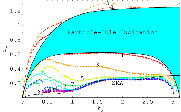
Figure 9: $k_{y}$-dependence of the plasma frequency $\omega_{p}(k_{x}=\pi/4,k_{y})$ for the RPA and the GRPA with the particle-hole excitation region and the phonon frequency. The number means the dimension of the matrix $\left[1-W^{\rm eff}(k)\pi^{(0)}({\bf k},\omega)\right]^{-1}$. The dashed line is the plasmon in the RPA, and the dotted line is the one in the GRPA. The solid line is the phonon derived in the SMA.SMA The behavior of $\omega_{p}$ approaches to the phonon one in the SMA when the matrix dimension increases. The particle-hole excitation region is unchanged and remains in the (G)RPA. The unit of $\omega_{p}(k_{x},k_{y})$, $k_{x}$ and $k_{y}$ is $q^{2}/(a\hbar)$, $1/(r_{s}a)$ and $r_{s}/a$, respectively.

III.5 Correlation energy

We calculate the (G)RPA correlation energy in this section. As is well known, the correlation energy is given by the virtual coupling constant $\lambda$ integrationfetter

$$E^{\rm total}=E^{\rm HF}+\int_{0}^{1}d\lambda\frac{1}{2}\int_{-\infty}^{\infty}\frac{d^{2}k}{(2\pi)^{2}}\tilde{V}({\bf k})\langle E(\lambda)|\;_{\circ}^{\circ}\;\tilde{\rho}({\bf k})\tilde{\rho}(-{\bf k})\;_{\circ}^{\circ}\;|E(\lambda)\rangle,$$ (18)

where $\tilde{\rho}({\bf k})=j^{0}({\bf k})$, $\tilde{V}({\bf k})=\frac{2\pi q^{2}}{|{\bf k}|}$ is the Fourier transformed Coulomb interaction, and $|E(\lambda)\rangle$ is the ground state for the system with the virtual coupling constant $\lambda$. The second term of Eq. (18) is the correlation energy. By replacing $\tilde{\rho}({\bf k})$ with $\tilde{\rho_{\ast}}({\bf k})$ and $\tilde{V}({\bf k})$ with $V_{l}({\bf k})$ in Eq. (18), the LL projected correlation energy is represented by a vNL basis:

$$E^{\rm corr} = \frac{1}{2}\int_{0}^{1}d\lambda\int_{-\infty}^{\infty}\frac{d^{2}k}{(2\pi)^{2}}V_{l}({\bf k})\langle E(\lambda)|\;_{\circ}^{\circ}\;\tilde{\rho_{\ast}}({\bf k})\tilde{\rho_{\ast}}(-{\bf k})\;_{\circ}^{\circ}\;|E(\lambda)\rangle$$ (19)

$$= \frac{1}{2}\int_{0}^{1}d\lambda\int_{\rm MBZ}\frac{d^{2}\hat{k}}{(2\pi)^{2}}\frac{d^{2}p_{1}}{(2\pi)^{2}}\frac{d^{2}p_{2}}{(2\pi)^{2}}\sum_{n}V_{l}({\bf k}+2\pi\tilde{{\bf n}})e^{-\frac{i}{2\pi}\hat{k}_{x}(p_{1}-p_{2})_{y}+i({\bf p}_{1}-{\bf p}_{2})\times{\bf n}}$$

$$\qquad\times\langle E(\lambda)|\;_{\circ}^{\circ}b_{l,{\bf p}_{1}+\hat{\bf k}}^{\dagger}b_{l,{\bf p}_{1}}b_{l,{\bf p}_{2}}^{\dagger}b_{l,{\bf p}_{2}+\hat{\bf k}}\;{}_{\circ}^{\circ}|E(\lambda)\rangle.$$

The integer $n$ is caused by dividing the $k$-integral region into summation of one MBZ. The RPA correlation energy is the sum of the chain diagram of bubble as shown in Fig. 10 which is derived by the perturbative calculation about the virtual coupling constant $\lambda$. The density correlation function part in Eq. (19) is calculated as

$$\int_{\rm MBZ}\frac{d^{2}p_{1}}{(2\pi)^{2}}\frac{d^{2}p_{2}}{(2\pi)^{2}}\sum_{n}V_{l}({\bf k}+2\pi\tilde{{\bf n}})e^{-\frac{i}{2\pi}\hat{k}_{x}(p_{1}-p_{2})_{y}+i({\bf p}_{1}-{\bf p}_{2})\times{\bf n}}$$ (20)

$$\qquad\times\langle E(\lambda)|\;_{\circ}^{\circ}b_{l,{\bf p}_{1}+\hat{\bf k}}^{\dagger}b_{l,{\bf p}_{1}}b_{l,{\bf p}_{2}}^{\dagger}b_{l,{\bf p}_{2}+\hat{\bf k}}\;{}_{\circ}^{\circ}|E(\lambda)\rangle$$

$$\stackrel{{\scriptstyle\rm RPA}}{{\simeq}} i\sum_{mnp}\pi^{(0)}_{mn}(k)W_{n}(k)\pi^{(0)}_{np}(k)\lambda W_{p}(k)\left(\frac{1}{1-\pi^{(0)}(k)\lambda W(k)}\right)_{pm}$$

Here $\pi^{(0)}_{nm}$ is given in Eq. (13). We take only the diagonal matrix elements contribution and approximate Eq. (20) as

$$i\,\sum_{n}(\pi^{(0)}_{nn}(k)W_{n}(k))^{2}\frac{\lambda}{1-\pi^{(0)}_{nn}(k)\lambda W_{n}(k)}.$$ (21)

Figure 10: The chain diagram for RPA correlation energy.

In the summation about $n$, the contribution of $n\geq 1$ terms are negligible because of the Gaussian factor in $V_{l}({\bf k})$. So we consider only the $n=0$ term. By substituting Eq. (21) into Eq. (19), the integral about $\lambda$ gives the RPA correlation energy $E_{\rm RPA}^{\rm corr}$ as

$$E_{\rm RPA}^{\rm corr}=-\frac{i}{2}\int_{-\infty}^{\infty}\frac{d\omega}{2\pi}\int_{\rm MBZ}\frac{d^{2}\hat{k}}{(2\pi)^{2}}\left\{\log{(\epsilon^{\rm RPA}({\bf k},\omega))}+\pi_{\rm 1-loop}(k_{y},\omega)W_{0}(k)\right\}.$$ (22)

The numerical estimates of $E^{\rm HF}$, the real part of $E_{\rm RPA}^{\rm corr}$ and the total energy $E^{\rm total}$ per particle at the half-filled $l=2$ LL are obtained as follows:

$$E^{\rm HF} = -0.7706,$$

$$E^{\rm corr}_{\rm RPA} = -0.0341,$$ (23)

$$E^{\rm total} = -0.8047,$$

where the energy unit is $\frac{q^{2}}{a}$. The total energy is lowered by the RPA correlation energy significantly.

Figure 11: The chain diagram for GRPA correlation energy.

GRPA correlation energy is the sum of the chain diagram of bubble and ladder as shown in Fig. 11. Corresponding to Eq. (21) in RPA, Eq. (20) is approximated in GRPA as

$$i\,\sum_{n}(\pi^{(0)}_{nn}(k))^{2}W_{n}({\bf k})W_{n}^{\rm eff}({\bf k})\frac{\lambda}{1-\pi^{(0)}_{nn}(k)\lambda W^{\rm eff}_{n}({\bf k})}.$$

Considering $n=0$ term, the GRPA correlation energy $E_{\rm GRPA}^{\rm corr}$ is written by $\pi_{\rm 1-loop}(k_{y},\omega)$ as

$$E_{\rm GRPA}^{\rm corr}=-\frac{i}{2}\int_{-\infty}^{\infty}\frac{d\omega}{2\pi}\int_{\rm MBZ}\frac{d^{2}\hat{k}}{(2\pi)^{2}}\left\{\left(\frac{W_{0}(k)}{W^{\rm eff}_{0}(k)}\right)\log{\left[1-W^{\rm eff}_{0}(k)\pi_{\rm 1-loop}(k_{y},\omega)\right]}+\pi_{\rm 1-loop}(k_{y},\omega)W_{0}(k)\right\}.$$ (24)

The numerical estimates of the real part of $E_{\rm GRPA}^{\rm corr}$ and the total energy $E^{\rm total}$ per particle at the half-filled $l=2$ LL are obtained as follows:

$$E^{\rm corr}_{\rm GRPA} = -0.0385,$$ (25)

$$E^{\rm total} = -0.8090.$$

GRPA correlation energy is slightly lower than RPA correlation energy.

Yoshioka calculated the corresponding HF energy for the ACDW state.daijiro The ACDW state has anisotropic energy gaps in $p_{x}$ and $p_{y}$-direction. Our striped Hall gas, on the other hand, has an energy gap only in $p_{y}$-direction. The numerical value of Yoshioka’s HF energy is $E^{\rm Y}=-0.7763$. Our total energy $E^{\rm total}$ of the ground state is smaller than $E^{\rm Y}$, hence our striped Hall gas including the quantum fluctuation at the (G)RPA level is more stable than the ACDW. On the other hand, Shibata and Yoshioka studied the ground state phase of 2D electrons in $l=2$ LL by a density matrix renormalization group (DMRG) method, which is a numerical calculation of a small system improved by the renormalization group method.Shibata The DMRG results seem to predict the striped Hall gas at the half-filled higher LL. The total energy given by the DMRG is $E^{D}=-0.796\pm 0.004$ Shibata_pri which is smaller than $E^{\rm Y}$, whereas it is close to $E^{\rm total}$.

The one-electron energy of the ACDW state has a gap in both $p_{y}$ and $p_{x}$ direction, whose value is about 1 K.bubble_fertig Hence, this state is insulator in $x$ and $y$ direction and the gap structure causes the quantization of the Hall conductance. However, experiments show the huge anisotropic resistivity and the Hall conductance is not quantized at several mK.Lilly ; Du Since the striped Hall gas has the anisotropic Fermi surface, the $x$ direction is insulator whose gap energy is the cyclotron energy, and the $y$ direction is metal in which the electron gas state realizes. Therefore the striped Hall gas is more consistent with experiments than ACDW. Moreover the comparison of the correlation energy with the ACDW and results of DMRG seems to support our striped Hall gas.

IV Summary

Using the one-loop polarization function which includes only intra-LL effects, the dielectric function, the plasma frequency, and correlation energy are calculated in the (G)RPA for the striped Hall gas. The characteristic feature of the plasma frequency is anisotropic gapless behavior. The anisotropy is due to the spontaneous breaking of rotational symmetry and the gapless feature comes from two-dimensionality of the system. The anisotropic plasma frequency will be observed by some experiments: e.g. a surface acoustic wave. The numerical result of GRPA plasmon suggests that the plasmon in the striped Hall gas is the same as phonon in the striped Hall gas which is the Nambu-Goldstone mode due to the the spontaneous breaking of translational symmetry. In contrast to the quantum Hall smecticAnna derived by edge current picture and TDHFA applying to the ACDW, this excitation state reflects the striped Hall gas state. It is shown that the quantum fluctuation effect for the striped Hall gas substantially reduces the total energy in (G)RPA. This means that the quantum fluctuation plays a important role in the striped Hall gas. The quantum Hall gas properties strongly depends on the electron self-energy with the anisotropic Fermi surface. The treatment for quantum fluctuation effects to the electron self-energy is beyond the scope of the present paper, and is very interesting as a future problem.

Appendix A Hartree-Fock approximation

In the intra-LL HFA, we reduce the Coulomb interaction term to the kinetic term by using a mean field $U(p)\equiv\langle{\rm HF}|b_{l}^{\dagger}({\bf p})b_{l}({\bf p})|{\rm HF}\rangle$ where $|\rm HF\rangle$ is a many-particle state satisfying a self-consistency equation. The interaction Hamiltonian projected into the $l$th LL,

$$H_{1}\stackrel{{\scriptstyle\rm project}}{{=}}\frac{1}{2}\int_{-\infty}^{\infty}\frac{d^{2}k}{(2\pi)^{2}}:\tilde{\rho_{\ast}}({\bf k})V_{l}(k)\tilde{\rho_{\ast}}(-{\bf k}):,$$

is approximated by the HF Hamiltonian

$$H^{\rm HF}=\frac{\nu^{\ast}}{N}\int_{\rm MBZ}\!\!\frac{d^{2}p}{(2\pi)^{2}}\frac{d^{2}p^{\prime}}{(2\pi)^{2}}v_{l}^{\rm HF}\!({\bf p}-{\bf p}^{\prime})U({\bf p}^{\prime})b_{l}^{\dagger}({\bf p})b_{l}({\bf p})-\frac{\nu^{\ast}}{2N}\int_{\rm MBZ}\!\!\frac{d^{2}p}{(2\pi)^{2}}\frac{d^{2}p^{\prime}}{(2\pi)^{2}}U({\bf p})v_{l}^{\rm HF}\!({\bf p}-{\bf p}^{\prime})U({\bf p}^{\prime}).$$ (26)

Here, we define

$$v_{l}^{\rm HF}({\bf p}-{\bf p}^{\prime})\equiv\sum_{n}\left\{V_{l}(2\pi\tilde{\bf n})e^{i({\bf p}-{\bf p}^{\prime})\times{\bf n}}-V_{l}(2\pi\tilde{{\bf n}}+\tilde{{\bf p}}^{\prime}-\tilde{\bf p})\right\}.$$ (27)

$\nu^{\ast}$ is a filling factor for the highest LL, and $N$ is a number of electrons at the highest LL. In this paper, $\nu^{\ast}$ is set to 1/2. The states below $l-1$ th LL are fully occupied. The first term in Eq. (27) is the Hartree potential and the second one is the Fock potential. The uniform positive background charge cancels the ${\bf n}=0$ term in the Hartree term. Since the state at the $l$th LL is occupied by electrons whose energy is below a Fermi energy $\mu_{\rm F}$, the mean field is written as $U({\bf p})=\frac{N}{\nu^{\ast}}\theta(\mu_{\rm F}-\epsilon_{l}^{\rm HF}({\bf p}))$. Hence, the self-consistency equation of one-electron energy $\epsilon_{l}^{\rm HF}({\bf p})$ reads

$$\epsilon_{l}^{\rm HF}({\bf p})=\int_{\rm MBZ}\frac{d^{2}p^{\prime}}{(2\pi)^{2}}v_{l}^{\rm HF}({\bf p}-{\bf p}^{\prime})\,\theta(\mu_{\rm F}-\epsilon_{l}^{\rm HF}({\bf p}^{\prime})\,).$$ (28)

The one-electron energy has a periodic structure $\epsilon_{l}^{\rm HF}({\bf p})=\epsilon_{l}^{\rm HF}({\bf p}+2\pi{\bf n})$ owing to $v_{l}^{\rm HF}({\bf p})=v_{l}^{\rm HF}({\bf p}+2\pi{\bf n})$.

Appendix B One-electron spectrum

The one-electron spectrum is given by the next explicit relation $\epsilon_{l}^{\rm HF}(p_{y})=\epsilon_{l}^{\rm H}(p_{y})+\epsilon_{l}^{\rm F}(p_{y})$, where

$$\epsilon_{l}^{\rm H}(p_{y}) = \frac{2q^{2}}{\pi}\sum_{n=0}^{\infty}V_{l}\!\left[\frac{2\pi(2n+1)}{r_{s}}\right]\frac{(-1)^{n}\cos[(2n+1)p_{y}]}{(2n+1)}$$ (29)

$$\epsilon_{l}^{\rm F}(p_{y}) = -r_{s}q^{2}\sum_{n=-\infty}^{\infty}\int_{-\frac{\pi}{2}}^{\frac{\pi}{2}}\frac{dk_{y}}{2\pi}\int_{-\infty}^{\infty}\!\!\!\frac{dk_{x}}{2\pi}\;V_{l}\!\left[\sqrt{k_{x}^{2}+r_{s}^{2}(k_{y}-p_{y}-2\pi n)^{2}}\right].$$ (30)

Appendix C Feynman rule

In the following calculation, the interaction picture is applied in perturbation theory. In the Heisenberg picture, the time-dependence of an operator $\mathcal{O}^{\rm H}(t)$ is defined as $\mathcal{O}^{\rm H}(t)=e^{iH_{1}t}\mathcal{O}e^{-iH_{1}t}$.

The electron Green’ function is defined by

$$\langle\Psi_{0}|{\rm T}b^{\rm H}_{{\bf p}_{1},t_{1}}b^{\dagger{\rm H}}_{{\bf p}_{2},t_{2}}|\Psi_{0}\rangle \equiv iG({\bf p}_{1},t_{1}-t_{2})\sum_{n}(2\pi)^{2}\delta^{(2)}({\bf p}_{1}-{\bf p}_{2}-2\pi{\bf n})e^{i\phi(p_{1},n)},$$ (31)

where $|\Psi_{0}\rangle$ is the exact ground state of $H_{1}$, and $\phi(p,n)=\pi(n_{x}+n_{y})-n_{y}p_{x}$. $\rm T$ means the time ordering. We write $b_{l}({\bf p},t)$ as $b_{{\bf p},t}$ and omit its LL index. The Heisenberg picture is changed to the interaction picture by using the relation $b_{{\bf k},t}^{\rm H}=S(0,t)b_{{\bf k},t}S(t,0)$, where $S(t,t^{\prime})=e^{iH^{\rm HF}t}e^{-iH_{1}t}e^{iH^{\rm HF}t^{\prime}}e^{-iH_{1}t^{\prime}}$. Using $S(t,t^{\prime})$ in Eq. (31), the Green function is written as a familiar form:

$$G({\bf k},t-t^{\prime})=-i\sum_{n=0}^{\infty}\frac{(-i)^{n}}{n!}\int_{-\infty}^{\infty}dt_{1}\cdots\int_{-\infty}^{\infty}dt_{n}\frac{\langle{\rm HF}|Tb_{{\bf k},t}b^{\dagger}_{{\bf k},t^{\prime}}V(t_{1})\cdots V(t_{n})|{\rm HF}\rangle}{\langle{\rm HF}|S(+\infty,-\infty)|{\rm HF}\rangle},$$ (32)

where the interaction $V(t)$ is the residual interaction in the interaction picture

$$V(t)=\frac{1}{2}\int_{-\infty}^{\infty}\!\!\!\frac{d^{2}k}{(2\pi)^{2}}\;_{\circ}^{\circ}\;\tilde{\rho_{\ast}}({\bf k},t)V_{l}(k)\tilde{\rho_{\ast}}(-{\bf k},t)\;_{\circ}^{\circ}\;.$$ (33)

The lowest order Green function is obtained as

$$G^{(0)}({\bf k},t-t^{\prime}) = -i\left\{\theta(t-t^{\prime})\theta(\epsilon_{\bf k}-\mu_{\rm F})e^{-i(t-t^{\prime})(\epsilon_{\bf k}-\mu_{\rm F})}-\theta(t^{\prime}-t)\theta(\mu_{\rm F}-\epsilon_{\bf k})e^{-i(t-t^{\prime})(\epsilon_{\bf k}-\mu_{\rm F})}\right\}.$$

Considering only intra LL effects, we omit the LL index and take the short notation of $\epsilon_{l}^{\rm HF}({\bf k})$ as $\epsilon_{\bf k}$. The Fourier transformation of the free propagator reads

$$\tilde{G}^{(0)}_{{\bf k},\omega} = \int_{-\infty}^{\infty}dt\;e^{i\omega t}G^{(0)}({\bf k},t)$$ (35)

$$= \frac{\theta(\epsilon_{\bf k}-\mu_{\rm F})}{\omega-\epsilon_{\bf k}+\mu_{\rm F}+i\delta}+\frac{\theta(\mu_{\rm F}-\epsilon_{\bf k})}{\omega-\epsilon_{\bf k}+\mu_{\rm F}-i\delta}.$$

In the vNL formalism, it is transparent way to represent the infinite ${\bf k}$-integral of Eq. (33) as the summation of one fundamental MBZ. So the residual interaction is written as

$$V(t)=\int_{\rm MBZ}\!\!\frac{d^{2}\hat{k}}{(2\pi)^{2}}\frac{d^{2}p_{1}}{(2\pi)^{2}}\frac{d^{2}p_{2}}{(2\pi)^{2}}e^{-\frac{i}{2\pi}\hat{k}_{x}p_{1y}}V_{l}(p_{1},k,p_{2})e^{\frac{i}{2\pi}\hat{k}_{x}p_{2y}}\>\;_{\circ}{}^{\circ}\>b_{t,{\bf p}_{1}+\hat{\bf k}}^{\dagger}b_{t,{\bf p}_{1}}b_{t,{\bf p}_{2}}^{\dagger}b_{t,{\bf p}_{2}+\hat{\bf k}}\>\;{}_{\circ}^{\circ}\>,$$ (36)

where we define

$$V_{l}(p_{1},k,p_{2}) \equiv \sum_{n=-\infty}^{\infty}V_{l}(k+2\pi\tilde{n})e^{i({\bf p}_{1}-{\bf p}_{2})\times{\bf n}}.$$ (37)

In stead of the infinite $k$-integral region, the infinite summation appears. The local interaction $V_{l}(k)$ in momentum space is replaced by the non-local one $V_{l}(p_{1},k,p_{2})$ including the phase factor in the density operator. For perturbative calculations, we use the Wick’s theorem and obtain an $n$-point correlation function for the interaction $V(t)$.

In the following we present the Feynman diagram rule in the momentum space for the perturbative residual interaction Eq. (36). The phase factor due to the magnetic field makes the vertex and the momentum conservation factors complicate.

(i) Draw a Feynman diagram. For an electron propagator, introduce the Green’s function

$$\tilde{G}^{(0)}_{{\bf p},\omega}=\begin{minipage}[h]{173.44534pt} \centerline{\hbox{\includegraphics[width=216.81pt]{a13.eps}}} \end{minipage}.$$ (38)

(ii) For one Coulomb line which is the interaction vertex, a local momentum interaction is not assigned in the usual way. We add a non-local interaction including four electron momentum ${\bf p}_{i}$ with phase factor as

$$V_{l}(p_{2},k,p_{3})e^{-\frac{i}{2\pi}\hat{k}_{x}(p_{1}-p_{4})_{y}}=\begin{minipage}[h]{173.44534pt} \centerline{\hbox{\includegraphics[width=216.81pt]{a14.eps}}} \end{minipage}.$$ (39)

(iii) Add a momentum conservation factor for each interaction vertices with four electron momentum ${\bf p}_{i}$ and frequency $\omega_{i}$

$$\sum_{nm}(2\pi)^{2}\delta({\bf p}_{1}-{\bf p}_{2}-\hat{\bf k}-2\pi{\bf n})e^{i\phi(p_{2},n)}\;(2\pi)^{2}\delta({\bf p}_{3}-{\bf p}_{4}+\hat{\bf k}-2\pi{\bf m})e^{i\phi(p_{3},m)}\\ \times(2\pi)^{2}\delta(\omega_{1}-\omega_{2}-\omega)\delta(\omega_{3}-\omega_{4}+\omega).$$ (40)

The phase factor $\phi(p_{i},n)$ is added to the delta function.

(iv) For one current vertex, a local momentum factor is also not assigned as the interaction vertex case. We add a non-local factor

$$g_{\mu}(k)e^{-\frac{i}{2\pi}\hat{k}_{x}p_{1y}+\frac{i}{4\pi}k_{x}k_{y}}=\begin{minipage}[h]{173.44534pt} \centerline{\hbox{\includegraphics[width=216.81pt]{a15.eps}}} \end{minipage}.$$ (41)

(v) Add a momentum conservation factor for each current vertices with two electron momentum ${\bf p}_{i}$ and frequency $\omega_{i}$

$$\sum_{n}(2\pi)^{2}\delta({\bf p}_{1}-{\bf p}_{2}-\hat{\bf k}-2\pi{\bf n})e^{i\phi(p_{2},n)}(2\pi)\delta(\omega+\omega_{1}-\omega_{2}).$$ (42)

The phase factor $\phi(p_{i},n)$ is added to the delta function.

(vi) Perform integral for internal momentum and add the numerical factor

$$\left\{\frac{1}{(2\pi)^{3}}\right\}^{I},$$ (43)

where $I$ is the number of internal line. Count the electron loop number and add the factor $(-1)^{L}$ for $L$ electron loops.

Appendix D Duality between the direct term and the exchange term

One of the surprising properties of the 2D electron system in a magnetic field is that the ladder diagrams take a similar form with the bubble diagram and the bubble and ladder diagrams can be summed up to the infinite order. This is caused by the duality between the direct term and the exchange term. In this section we show this property in the two-loop order as shown in Fig. 12.

Following the rule of Appendix C, the left two-loop diagram in Fig. 12 reads

$$-\sum_{n}\int\frac{d\omega_{1}}{2\pi}\frac{d\omega_{2}}{2\pi}\int_{\rm MBZ}\frac{d^{2}p_{1}}{(2\pi)^{2}}\frac{d^{2}p_{2}}{(2\pi)^{2}}\;\;\tilde{G}^{(0)}_{p_{1}-\hat{k},\omega_{1}-\omega}\tilde{G}^{(0)}_{p_{1},\omega_{1}}\tilde{G}^{(0)}_{p_{2}-\hat{k},\omega_{2}-\omega}\tilde{G}^{(0)}_{p_{2},\omega_{2}}V_{l}(\tilde{p}_{1}-\tilde{p}_{2}+2\pi\tilde{n})e^{\frac{i}{2\pi}({\bf p}_{1}-{\bf p}_{2}+2\pi{\bf n})\times\hat{\bf k}}$$ (44)

In general, the Fourier transform $\tilde{V}_{l}({\bf q})=\int\frac{d^{2}p}{(2\pi)^{2}}V_{l}({\bf p})e^{i{\bf p}\cdot{\bf q}}$ satisfies the following duality relation between the direct term and the exchange term,

$$\sum_{n}V_{l}({\bf p}+2\pi{\bf n})e^{i({\bf p}+2\pi{\bf n})\cdot{\bf q}}=\sum_{n}\tilde{V}_{l}({\bf q}+{\bf n})e^{-i{\bf p}\cdot{\bf n}}.$$ (45)

Using this relation, Eq. (44) is written as

$$-\sum_{n}\int\frac{d\omega_{1}}{2\pi}\frac{d\omega_{2}}{2\pi}\int_{\rm MBZ}\frac{d^{2}p_{1}}{(2\pi)^{2}}\frac{d^{2}p_{2}}{(2\pi)^{2}}\;\;\tilde{G}^{(0)}_{p_{1}-\hat{k},\omega_{1}-\omega}\tilde{G}^{(0)}_{p_{1},\omega_{1}}\tilde{G}^{(0)}_{p_{2}-\hat{k},\omega_{2}-\omega}\tilde{G}^{(0)}_{p_{2},\omega_{2}}\tilde{V}_{l}\!\!\left(\frac{k_{y}}{2\pi}+\tilde{n}_{y},-\frac{k_{x}}{2\pi}-\tilde{n}_{x}\right)e^{i{\bf n}\times({\bf p}_{1}-\bf{p}_{2})}$$ (46)

$$= -\sum_{n}\pi_{0n}(k)\tilde{W}_{n}(k)\pi_{n0}(k).$$

This result is equivalent to two bubbles connected with the interaction ${\tilde{W}}(k)$ as the right two-loop diagram in Fig. 12.

Figure 12: The two-loop ladder diagram and corresponding two-loop bubble diagram

References

• (1) M. P. Lilly, K. B. Cooper, J. P. Eisenstein, L. N. Pfeiffer, and K. W. West, Phys. Rev. Lett. 82, 394 (1999).
• (2) R. R. Du, D. C. Tsui, H. L. Stormer, L. N. Pfeiffer, K. W. Baldwin, and K. W. West, Solid State Commun. 109, 389 (1999).
• (3) A. A. Koulakov, M. M. Fogler, and B. I. Shklovskii, Phys. Rev. Lett. 76, 499 (1996); M. M. Fogler, A. A. Koulakov, and B. I. Shklovskii, Phys. Rev. B 54, 1853 (1996).
• (4) R. Moessner and J. T. Chalker, Phys. Rev. B 54, 5006 (1996).
• (5) N. Maeda, Phys. Rev. B 61, 4766 (2000).
• (6) T. Aoyama, K. Ishikawa and N. Maeda, Eurphys. Lett. 59, 444 (2002); D. Yoshioka, J. Phys. Soc. Jpn. 70, 2836 (2001).
• (7) K. Ishikawa, T. Aoyama, Y. Ishizuka and N. Maeda, Int. J. of Mod. Phys. B 17, 4765 (2003)
• (8) R. CΓ΄tΓ© and H. A. Fertig, Phys. Rev. B 62, 1993 (2000).
• (9) A. H. MacDonald and M. P. A. Fisher, Phys. Rev. B 61, 5724 (2000); A. Lopatnikova, S. H. Simon, B. I. Halperin, and X. G. Wen, ibid. 64, 155301 (2001); D. G. Barci, E. Fradkin, S. A. Kivelson, and V. Oganesyan, ibid. 65, 245319 (2002); D. G. Barci and E. Fradkin, ibid. 65, 245320 (2002).
• (10) T. Aoyama, K. Ishikawa, Y. Ishizuka and N. Maeda, Phys. Rev. B 66, 155319 (2002)
• (11) M. Gell-Mann and K. Brueckner, Phys. Rev. 106, 364 (1957).
• (12) K. Ishikawa, N. Maeda, T. Ochiai, and H. Suzuki, Physica E 4, 37 (1999); N. Imai, K. Ishikawa, T. Matsuyama, and I. Tanaka, Phys. Rev. B 42, 10610 (1990).
• (13) I. L. Aleiner and L. I. Glazman, Phys. Rev. B 52, 11296 (1995).
• (14) K. Ishikawa, N. Maeda, and T. Ochiai, Phys. Rev. Lett. 82, 4292 (1999); K. Ishikawa and N. Maeda, Physica B 298, 159 (2001); cond-mat/0102347.
• (15) R. CΓ΄tΓ© and A. H. MacDonald, Phys. Rev. B 44, 8759 (1991)
• (16) A. L. Fetter and J. D. Waleca, Quantum Theory of Many Particle Systems (McGraw-Hill, New York, 1971); G. D. Mahan, Many-Particle Physics (Plenum, New York, 2000)
• (17) D. Yoshioka, J. Phys. Soc. Jpn. 70, 2836 (2001).
• (18) N. Shibata and D. Yoshioka, Phys. Rev. Lett. 86, 5755 (2001)
• (19) N. Shibata (private communication).
• (20) This value is estimated from the single-particle density of states at $\nu^{\ast}=0.430$ for a few tesla, in R. CΓ΄tΓ©, C. Doiron, J. Bourassa and H. A. Fertig, cond-mat/0304412