Macroscopic quantum bound states of Bose Einstein condensates in optical lattices

Abstract

We discuss localized ground states of the periodic Gross-Pitaevskii equation in the framework of a quantum linear Schrödinger equation with effective potential determined in self-consistent manner. We show that depending on the interaction among the atoms being attractive or repulsive, bound states of the linear self consistent problem are formed in the forbidden zones of the linear spectrum below or above the energy bands. These eigenstates are shown to be exact solitons of the GPE equation. The implications of this bound state interpretation on the existence of a delocalization transition for multidimensional solitons is briefly discussed.

PACS numbers: 03.75.Fi, 05.30.Jp, 05.45.-a

One interesting phenomenon occurring in periodic nonlinear systems is the possibility to stabilize localized excitations as a result of the interplay between periodicity and nonlinearity. An example of this is provided by the nonlinear Schrödinger equation (NLS) with periodic potential. It is well known that the defocusing NLS does not admit bright soliton solutions, these being unstable against background decay [1]. The presence of a periodic potential, however, allows to stabilize bright solitons against decay, a phenomenon which is presently investigated in connection with Bose Einstein condensates (BEC) in optical lattices (OL). The possibility to form bright solitons in repulsive BEC with OL was analytically and numerically demonstrated, both for a discrete version of the NLS describing BEC arrays in the tight-binding approximation [2] and for the Gross-Pitaevskii equation (GPE) describing the properties of a continuous BEC in the mean field approximation [3, 4, 5]. The mechanism underlying soliton formation in periodic structures was identified to be the modulational instability of the Bloch states at the edges of the Brillouin zone [4]. These localized excitations correspond to states with energies inside the gaps of the underlying linear band structure (in nonlinear optics they are called gap solitons) and with an effective mass which depends on the sign of the interaction (for repulsive interactions, bright solitons have negative effective mass, this explaining their existence in BEC with OL [4, 6]). The usage of linear concepts such as Bloch states, effective mass, etc. [4, 6, 7], makes natural to ask whether nonlinear states could be interpreted in a pure linear (quantum mechanical) context.

The aim of the present paper is to address this problem by showing that soliton solutions of the periodic nonlinear Schrödinger equations correspond to bound states of the linear Schrodinger equation with an effective potential which can be determined in self-consistent (SC) manner. This problem will be discussed on the physical example of a Bose Einstein condensate in an optical lattice (OL) described, in mean field approximation, by the following normalized Gross-Pitaevskii equation

$$i\psi_{t}=\left[-\nabla^{2}+U_{ol}({\bf{x}})+\chi|\psi|^{2}\right]\psi$$ (1)

where $\chi$ is the nonlinear parameter, $\bf x$ denotes three dimensional coordinates and $U(\bf x)$ is a periodic potential representing the OL. To discuss bound state features of solitons we restrict to the one dimensional case (the approach however is of general validity and can be applied to NLS type equations in arbitrary dimensions). At the end of the paper we will briefly discuss the implications of the bound state interpretation of localized solutions on the soliton delocalization transition observed in higher dimensions [8]. We remark that the properties of solitons of the GPE in optical lattices were studied in [5] in terms of orbits of a chaotic system. Self-consistent approaches were also used as numerical tools to study discrete breathers of the discrete NLS [10] and the stability of gap solitons [9]. The physical implications and the full potentiality of the SC approach, however, have not been investigated.

Our analysis is based on the simple observation that the stationary localized ground states $\psi_{s}(x,t)=\psi(x)\exp(-\mu t)$ of the GPE (and more generally of any nonlinear Schrödinger-like equation) can be obtained by solving in a self-consistent manner the following linear Schrödinger problem

$$\left[-\nabla^{2}+\hat{V}_{eff}(x)\right]\psi=E\psi$$ (2)

with the effective potential

$$\hat{V}_{eff}=\hat{U}_{ol}(x)+\hat{U}_{s}(x)=A\cos(2x)+\chi|\hat{\psi}_{s}(x)|^{2}.$$ (3)

Here $\hat{U}_{ol}\equiv A\cos(2x)$ is the OL and $\hat{U}_{s}$ is the potential associated with a given eigenstate of the quantum problem (2). For a self-consistent solution, one starts with a trial wavefunction for $\psi_{s}$ (typically a gaussian waveform), calculates the effective potential and solves the corresponding eigenvalue problem (2). Then, one selects a given eigenstate (for example the ground state but not necessarily) as new trial function and iterates the procedure until convergence is reached.

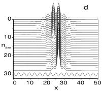
FIG. 1.: Panel (a) Energy spectrum for the effective potential (3) with $A=3$ and $\chi=0$ (Mathieu equation). Full lines represent exact values of the band edges of the Mathieu equation while dots are the eigenvalues obtained with the above procedure on a lattice of length $L=40\pi$, with $N=512$ points. Panel (b) Lowest energy band for the effective potential in Eq. (3) with $\psi_{s}$ taken as the ground state of the system and for $\chi=-1$ (attractive case). Parameters are fixed as in panel (a). Panel (c) The same as in panel (b) but for $A=-3$. Panel (d) Transition from the metastable IS mode to the OS ground state corresponding to the lower level of panel (c). The optical lattice (scaled by a factor 3) is reported as an help to locate the symmetry center of the solutions. Parameters are fixed as in panel (c).

The problem is thus reduced to the diagonalization of the quantum Hamiltonian

$$\hat{H}=\hat{H}_{0}+\hat{V}_{eff}(x)$$ (4)

with $\hat{H}_{0}\equiv-\nabla^{2}$ the kinetic energy operator. This can be effectively done by adopting a discrete coordinate space representation $\{x_{n}=na\}$, $n=1,...,N$, with $a=L/N$ the discretization constant, $L$ the size of the system and N the total number of points. A basis for this space is simply a basis of $R^{N}$, i.e. the set of N-component vectors of the type $|n\rangle=(0,...0,1,0,...,0)$, with the $1$ in the position $n$. The effective potential is obviously diagonal in this representation i.e. $\langle n|\hat{V}_{eff}|n^{\prime}\rangle=V_{eff}(na)\delta_{n,n^{\prime}}$, while $\hat{H}_{0}$ is diagonal in the reciprocal representation $|k_{n}\rangle$, ($k_{n}=2\pi/Ln$, the two representations being related by the Fourier transform (unitary transformation). The matrix elements of the Hamiltonian $\hat{H}$ can then be constructed as

$$\langle n|\hat{H}|n^{\prime}\rangle\equiv H_{n,n^{\prime}}=\langle n|\hat{F}^{-1}\hat{H}_{0}\hat{F}|n^{\prime}\rangle+V_{eff}(na)\delta_{n,n^{\prime}}$$ (5)

where $\hat{F}|n\rangle$ denotes the Fourier transform of the vector $|n\rangle$.

FIG. 2.: Wavefunctions and corresponding effective potential for the bound states below the lowest bands of Fig 1a for attractive interaction $\chi=-1$. Panel (a). OS mode and corresponding effective potential for $E=-1.1667950$ (ground state) and $A=3$. The effective potential was scaled by a factor 6 for graphical convenience. Panel (b). Same as (a) for the IS mode at $E=-1.0485745$ and $A=-3$. Panel (c). Same as (a) for the OA mode. $E=-0.999261$. Panel (d). Same as (b) for the IA mode. $E=-0.9947127$. (e) Energy levels of the OS, IS, OA, IA, nodes inside the gap between the first two bands. The continuous line denotes the lower edge of the second band of Fig. 1a while the dotted lines denote the degenerate levels. Parameters are fixed as for corresponding modes in panels a-d. (f). Wavefunctions associated to the levels in panel e. For graphical convenience the IS mode was shifted by -1.0 down while the IA and OS modes were shifted up by 0.5 and 1.0, respectively.

For an effective construction of these matrix elements one can use the fast Fourier transform while for the computation of the spectrum one can recourse to standard numerical routines for the diagonalization of real symmetric matrices. To check the method we consider first the case of a linear effective potential of the form $V_{eff}=U_{ol}=A\cos(2x)$ for which the eigenvalue problem reduces to the well known Mathieu equation. In Fig. 1a we depict the lowest part of the spectrum (notice that in this case there is no SC procedure due to the linearity of the problem) from which we see the appearance of a band structure with band edges which exactly coincide with the values obtained for the Mathieu equation (for high energy bands to get good accuracy one needs to increase $N$). In this paper we are mainly interested in the localized states associated with the lowest two bands (i.e., the ones physically most relevant), and for this purpose the choice of $N=256$ will be adequate for most of the calculations.

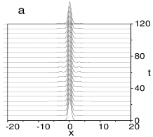
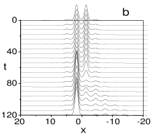
FIG. 3.: Panel (a). Time evolution of the OS bound state of Fig 2a as obtained from GPE. Panel (b). Same as in panel (a) for the IS mode of Fig. 2c.

FIG. 4.: Energy spectrum in correspondence of the localized states above the lowest band of Fig. 1a for repulsive interactions $\chi=1$. Panel (a). Spectrum associated to the OS mode. Parameters are $A=-3,N=256,L=40\pi$. Panel (b). Same as panel (a) but for the IA mode with $A=3$. The continuous lines denote exact band edges of the Mathieu equation.

In Fig. 1b we show how the lowest band of panel 1a is modified by the nonlinear potential $V_{eff}(x)=A\cos(2x)+\chi|\psi_{0}|^{2}$, where $\psi_{0}$ is taken to be the ground state of the system, for the case $\chi<0$ (negative scattering length). A bound state below the band which rapidly converges to a constant value is quite evident. One can see that the state forms from the lower edge of the band and is accompanied by a rearrangement of the extended states inside the band. The corresponding eigenvector is depicted in Fig.2a together with its effective potential. Notice that the potential has an attractive character (potential well) and the bound state is symmetric around a minima of the OL, i.e., it resembles the onsite-symmetric intrinsic localized mode (ILM) of nonlinear lattices (NL) [11]. In the following we shall call it the onsite symmetric (OS) bound state. By shifting the phase of the OL by $\pi$ (i.e. by changing the sign of $A$) one obtains an eigenstate centered on maxima instead than on minima. This bound state is depicted in Fig. 2b and in analogy with NL we shall call it the intersite symmetric (IS) mode. The corresponding spectrum is reported in Fig. 1c. Notice that the IS mode corresponds to the plateau formed just before the decay into the OS mode occurs as shown in panel 1d (also note the appearance of an intersite-symmetric (IA) excited level in Fig. 1c which is absorbed into the band in correspondence of the IS-OS decay).

FIG. 5.: Wavefunctions and effective potentials of the bound states levels of Fig. 4 a,b, for the repulsive case $\chi=1$. Panel (a). OS mode with corresponding effective potential (thin line). Energy is $E=-0.078355$ and $A=-3$. Panel (b). Same as in Panel (a) for the IA mode. $E=-0.376645$, $A=3$. Panel (c). Same as in panel (a) for the OA mode. $E=-0.683070$. Panel (d). Same in panel (b) for the IS mode. $E=-0.691676$. Parameters are fixed as $N=256$, $L=40\pi$ for panels (a), (b), and $N=512$, $L=40\pi$ for panels (c), (d). The effective potentials have been reduced by a factor $6$ for graphical convenience.

We have checked that these bound states coincide with the ones obtained with the approach of Ref. [5] for the same values of energy. The stability of the OS mode and the decay of the IS mode into the OS state was checked by direct numerical integrations of the GPE (see Fig.3). To obtain the onsite asymmetric (OA) mode one needs to take the first excited state $\psi_{1}$ as effective potential in the SC procedure. This indeed produces an exact soliton solution of the GPE of type OA as shown in Fig.2c. A shifting of the potential by $\pi$ produce the intersite asymmetric (IA) mode of Fig. 2d. These solutions have the same energies and are more unstable than the IS mode (they, however, do not decay into the ground state but get mixed with the extended states in the band). In general, the effective potentials can be taken of the form $\hat{V}_{eff}=\hat{V}_{ol}+\chi|\hat{\psi}_{n}(x)|$ with $\psi_{n}$ the n-th eigenstate of the eigenvalue problem in (2). If the energy of $\psi_{n}$ lies outside the bands a localized mode of the type described above is produced, while if it lies inside a band, extended states which are nonlinear analogue of the Bloch states [7], are produced. From this we conclude that both localized and extended solutions of the GPE are exact quantum eigenstates of the Schrödinger equation with a suitable effective potential. From the above analysis one expects that below each higher energy bands, eigenstates of the same symmetry type as the ones found for the lowest band should exist. This is precisely what we show in Fig.s 2e, 2f for the energy spectrum and the corresponding eigenstated in the gap below the second band.

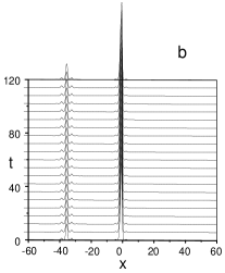
FIG. 6.: Panel (a). Two soliton bound state of the repulsive GPE obtained from the SC procedure by using as effective potential $V_{eff}=V_{ol}+|\frac{1}{2}\psi_{1}-\psi_{2}]^{2}$ where $\psi_{1},\psi_{2}$ denote two eigenfunctions at the top of the first band. Panel (b). Time evolution (modulo square) of the bound state in panel (a) taken as initial condition for the integration of the full GPE.

Notice that the OA and the IS eigenstates are degenerated (the same occurs also to the OS and IA modes). The OA and IS bound states are both very stable while the energy levels of the OA and IS modes, after establishing a plateau similar to the one in Fig 1c, become unstable (the energy oscillates between this level and the lower edge of the second band). The instability of these modes can be understood as an hybridization of the state (being very close to the band edge) with extended states of the second band and is confirmed by direct numerical integration of the PDE system.

Similar localized modes can be found also for repulsive interactions ($\chi>0$), the main difference with the previous case being that now the states appear in the gap above the band edges instead than below. This is shown in Fig. 4 for the lowest energy levels inside the first gap. The corresponding eigenvectors are shown in Fig.5 together with their effective potentials. Notice that the potential has a local repulsive character (it increases in correspondence of the states) so that these bound states could not exist without the OL. We remark that localized modes similar to the ones described in this paper were found also in atomic-molecular BEC using an approach based on Wannier functions [12].

Besides localized and extended states, the SC procedure allows to construct full nonlinear bands in reciprocal space (we omit details for brevity). It is worth remarking that more complicated set of solutions of the GPE can be constructed with the SC procedure by taking as effective potentials linear combinations of eigenstates. An example of this is shown in Fig.6 for the case of repulsive interaction. We see that a linear combination of two eigenstates leads to a bound state with two humps which corresponds to a multi-soliton solution of the GPE (see panel b). This is a general property and we conjecture that all solutions of the periodic GPE (and more in general of the NLS-like equations with arbitrary potentials) can be obtained with the SC method taking all possible combinations of linear eigenstates as effective potentials.

Before closing this paper we wish to remark that the above bound state interpretation has important consequences on the delocalizing transition [8] of localized solutions of the GPE in OL. Since in a 1D potential bound state always exists, it follows from the above analysis that no delocalizing transition of a BEC soliton can occur in this case. On the contrary, for $D\geq 2$ a finite potential depth is required to form a bound state, this implying that a soliton delocalization transition can occur. A detailed investigation of the delocalizing transition of BEC solitons in OL will be reported elsewhere [13].

It is a pleasure to thank Prof. S. De Filippo and Dr. B. Baizakov for interesting discussions. Financial support from a MURST-PRIN-2003 Initiative, and from the European grant LOCNET no. HPRN-CT-1999-00163, is also acknowledged.

REFERENCES

- [1] Alwyn Scott Nonlinear Science: Emergence and Dynamics of Coherent Structures, Oxford Univ. Press, 1999.
- [2] A. Trombettoni and A. Smerzi, Phys. Rev. Lett. 86, 2353 (2001); F. K. Abdullaev, B. B. Baizakov, S. A. Darmanyan, V. V. Konotop, and M. Salerno, Phys. Rev. A 64, 043606 (2001).
- [3] S. Pötting, O. Zobay, P. Meystre, and E. M. Wright, J. Mod. Opt. 47, 2653 (2000).
- [4] V. V. Konotop and M. Salerno, Phys. Rev. A 65, 021602 (2002); A. Smerzi, A. Trombettoni, P.G. Kevrekidis, A.R. Bishop, Phys.Rev. Lett. 89. 17042 (2002).
- [5] G. L. Alfimov, V. V. Konotop, and M. Salerno, Europhys. Lett. 58, 7 (2002); N.K. Efremidis and D. N. Christodoulides, Phys.Rev.A 67 063608 (2003).
- [6] M. J. Steel and W. Zhang, e-print cond-mat/9810284.
- [7] D. Diakonov, L.M. Jensen, C.J. Pethick, and H. Smith, Phys.Rev. A 66 013604 (2002); P.J. Louis, E.A. Ostrovskaya C.M. Savage, and Y.S. Kivshar, e-print cond-mat/0208516
- [8] G. Kalosakas, K. Ø. Rasmussen, and A. R. Bishop, Phys. Rev. Lett. 89, 030402 (2002); see also S. Flach, K. Kladko, and R.S. MacKay, Phys. Rev. Lett. 78, 1207 (1997).
- [9] Karen Marie Hilligsœ, Markus K. Oberthaler, and Karl-Peter Marzlin, Phys. Rev. A 66, 063605 (2002).
- [10] P.G. Kevrekidis, K.O Rasmussen, A.R. Bishop, Phys. Rev. E 61, 4652 (2000)
- [11] A.J. Sievers and S. Takeno, Phys.Rev.Lett. 61, 970 (1988); O.M. Braun and Yu. S. Kivshar, Phys.Rep. 306, 2 (1998).
- [12] F.Kh. Abdullaev and V.V. Konotop, Phys. Rev. A 68 013605 (2003).
- [13] B. B. Baizakov, M. Salerno, Phys. Rev. A 2003 (in press).