Power and Heat Fluctuation Theorems for Electric Circuits

Abstract

Using recent fluctuation theorems from nonequilibrium statistical mechanics, we extend the theory for voltage fluctuations in electric circuits to power and heat fluctuations. They could be of particular relevance for the functioning of small circuits. This is done for a parallel resistor and capacitor with a constant current source for which we use the analogy with a Brownian particle dragged through a fluid by a moving harmonic potential, where circuit-specific analogues are needed on top of the Brownian-Nyquist analogy. The results may also hold for other circuits as another example shows.

Nanotechnology is quickly getting within reach, but the physics at these scales could be different from that at the macroscopic scale. In particular, large fluctuations will occur, with mostly unknown consequences. In this letter, we will investigate properties of electric circuits concerning the fluctuations of power and heat within the context of the so-called Fluctuation Theorems (FTs). These theorems were originally found in the context of non-equilibrium dynamical systems theory. Surprisingly, these can be applied also to electric circuits, as we will show, and thus give further insight into their behavior.

Let us first give a brief introduction to the FTs. First found in dynamical systemsEvansetal93 ; GallavottiCohen95a and later extended to stochastic systemsKurchan98 , these conventional FTs give a relation between the probabilities to observe a positive value of the (time averaged) “entropy production rate” and a negative one. This relation is of the form $P(\sigma)/P(-\sigma)=\exp[\sigma\tau]$, where $\sigma$ and $-\sigma$ are equal but opposite values for the entropy production rate, $P(\sigma)$ and $P(-\sigma)$ give their probabilities and $\tau$ is the length of the interval over which $\sigma$ is measured. In these systems, the above mentioned FT is derived for a mathematical quantity $\sigma$, which has a form similar to that of the entropy production rate in Irreversible Thermodynamics.

Apart from an early experiment in a turbulent flowotherexperiment , for quite some time, the investigations of the FTs were restricted to theoretical approaches and simulations. In 2002, Wang et al. performed an experiment on a micron-sized Brownian particle dragged through water by a moving optical tweezer. In this experiment, a Transient Fluctuation Theorem (TFT) was demonstrated for fluctuations of the total external work done on the system in the transient state of the system, i.e., considering a time interval of duration $\tau$ which starts immediately after the tweezer has been set in motionWangetal02 . In contrast, a Stationary State Fluctuation Theorem (SSFT), which was not measured, would concern fluctuations in the stationary state, i.e., in intervals of duration $\tau$ starting at a time long after the tweezer has been set in motion. While the work fluctuations satisfy the conventional TFT and SSFTMazonkaJarzynski99 ; VanZonCohen02b , the heat fluctuations satisfy different, extended FTs due to the interplay of the stochastic motion of the fluid with the deterministic harmonic potential induced by the optical tweezerVanZonCohen03a ; VanZonCohen03b . Given the possible problems with identifying the entropy productionWangetal02 ; MazonkaJarzynski99 , in this letter we prefer to consider the work and the heat.

We remark that the conventional FTs hold in time-reversible, chaotic dynamical systemsEvansetal93 ; GallavottiCohen95a and in finite stochastic systems if transitions can occur forward and backwardKurchan98 . However, the general condition for an extended FT is unknown.

In view of the well-known analogy of Brownian motion (as in the experiment of Wang et al.) and Nyquist noise in electric circuitsVanKampenMazo , one could ask whether the TFT and SSFT based on the Langevin equation also apply to electric circuits. Electric circuits are interesting as they are directly relevant to nanotechnology and because they lend themselves easily to experiments. Indeed, it turns out the conventional FTs hold for work and the extended FTs for heat, as we will show here. We emphasize that to connect with previous papers on which this one is based, we will also use the term work for the electric circuits, which is nothing but the time integral of the power.

To exploit the analogy of the Langevin descriptions for electric circuit and that of the Brownian particle, we first recall the form of the Langevin equation for the Brownian particle in the experiment of Wang et al.VanZonCohen02b :

$$m\frac{d^{2}x_{t}}{dt^{2}}=-\alpha\frac{dx_{t}}{dt}+\xi_{t}-k(x_{t}-v^{*}t).$$ (1)

Here, $m$ is the mass of the Brownian particle, $x_{t}$ is its position at time $t$, $\alpha$ is the (Stokes’) friction coefficient, $k$ is the strength of the harmonic potential induced by the optical tweezer, and $v^{*}$ is the constant speed at which the tweezer is moved. $\xi_{t}$ represents a Gaussian white noise which satisfies

$$\langle\xi_{t}\rangle=0;\quad\langle\xi_{t}\xi_{t^{\prime}}\rangle=2k_{B}T\alpha\,\delta(t-t^{\prime}),$$ (2)

where $\langle\rangle$ denotes an average over an ensemble of similar systemsVanKampenMazo , $T$ is the temperature of the water and $k_{B}$ is Boltzmann’s constant. Usually, the velocity relaxes quickly, so one can set $m=0$ in Eq. (1).

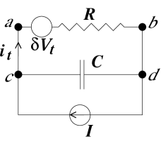
Figure 1: Circuit with Nyquist noise and a resistor and capacitor in parallel, subject to a current source.

Next we consider in Fig. 1 an electric circuit in which a resistor with resistance $R$ and a capacitor with capacitance $C$ are arranged in parallel and are subject to a constant, nonfluctuating current source $I$. Energy is being dissipated in the resistor and according to the fluctuation-dissipation theorem this means there are fluctuations too. To a good approximation, one can use a Gaussian random noise term $\delta V_{t}$ to describe these fluctuationsVanKampenMazo , which is depicted in the figure by a voltage generator. In addition, we define $q_{t}$ as the charge that has gone through the resistor, $i_{t}$ as the current that is going through it (so $i_{t}=dq_{t}/dt$) and $q^{\prime}_{t}$ as the charge on the capacitor, all at time $t$. Using that $q_{t}^{\prime}=\int_{0}^{t}dt^{\prime}\,(I-i_{t^{\prime}})=It-q_{t}$ and that $V_{ab}=q^{\prime}_{t}/C$, standard calculations for electric circuits give

$$0=-R\frac{dq_{t}}{dt}-\delta V_{t}-\frac{q_{t}-I\,t}{C},$$ (3)

in which $\delta V_{t}$ satisfiesVanKampenMazo

$$\langle\delta V_{t}\rangle=0;\quad\langle\delta V_{t}\delta V_{t^{\prime}}\rangle=2k_{B}TR\,\delta(t-t^{\prime}).$$ (4)

We see that Eqs. (3) and (4) are of a very similar form as those for a one-dimensional massless Brownian particle dragged through a fluid by means of a harmonic potential in Eqs. (1) and (2)footnote11 . Table 1 gives all the analogues, i.e., both the well-known Brownian motion-Nyquist noise ones ($\xi_{t}$, $\alpha$, $T$ vs. $\delta V_{t}$, $R$, $T$) as well as additional circuit-specific ones.

Brownian particle RC circuits $\xi_{t}$ $-\delta V_{t}$ $\alpha$ $R$ $T$ $T$ $x_{t}$ $q_{t}$ $v_{t}$ $i_{t}$ $k$ $1/C$ $v^{*}$ $\>I$ (or $CA$ in the serial case)

Table 1: The analogy of a circuit and a Brownian particle.

Given this analogy, we turn to the heat fluctuations in this circuit. This heat is developed in the resistor. Thus, the dissipated heat over a time $\tau$ is given by the time integral of the voltage over the resistor, $V_{ab}$, times the current through it, $i_{t}$, i.e.,

$$Q_{\tau}=\int_{0}^{\tau}dt\,i_{t}[i_{t}R+\delta V_{t}]=-\int_{0}^{\tau}dt\,i_{t}\frac{q_{t}-It}{C},$$ (5)

where we used Eq. (3). This is precisely the quantity found in Refs. VanZonCohen03a ; VanZonCohen03b for the Brownian particle, when we use the analogies in Table 1. Hence $Q_{\tau}$ in this parallel RC circuit behaves completely analogous to the heat for the Brownian particle and thus we know that it satisfies the extended FT. That is, defining a fluctuation function by

$$f^{\mbox{\tiny$Q$}}_{\tau}\equiv\frac{k_{B}T}{\langle Q_{\tau}\rangle}\ln\left[\frac{P(+Q_{\tau})}{P(-Q_{\tau})}\right]$$ (6)

and a scaled heat fluctuation by $p_{\mbox{\tiny$Q$}}\equiv Q_{\tau}/\langle Q_{\tau}\rangle$, one has for large $\tau$

$$f^{\mbox{\tiny$Q$}}_{\tau}(p_{\mbox{\tiny$Q$}})=\left\{\begin{array}[]{ll}p_{\mbox{\tiny$Q$}}+O(\tau^{-1})&\mbox{if $0<p_{\mbox{\tiny$Q$}}<1$}\\ p_{\mbox{\tiny$Q$}}-\frac{1}{4}(p_{\mbox{\tiny$Q$}}-1)^{2}+O(\tau^{-1})&\mbox{if $1<p_{\mbox{\tiny$Q$}}<3$}\\ 2+O\left(\sqrt{(p_{\mbox{\tiny$Q$}}-3)/\tau}\right)&\mbox{if $p_{\mbox{\tiny$Q$}}>3$}.\\ \end{array}\right.$$ (7)

Here, we only gave the orders of magnitude of the finite-$\tau$ correction terms. Their detailed forms — which differ in the transient and the stationary state — require an involved calculation using the saddle-point method which can be found in Ref. VanZonCohen03b . Note that these calculations need not be redone for the current case but that we can make the substitutions in Table 1 and consider the one-dimensional case as can be obtained from footnote 24 of Ref. VanZonCohen03b .

Next, we discuss the work fluctuations in this circuit. The total work done in the circuit is the time integral of the power. The power is the current through the circuit, $I$, times the voltage over the whole circuit, $V_{cd}$, so that

$$W_{\tau}=\int_{0}^{\tau}dt\,I\left[-\frac{q_{t}-It}{C}\right].$$ (8)

This happens to be precisely the form of the work as we found in the Brownian caseVanZonCohen02b , if we use Table 1. This is somewhat surprising because those analogues were based on Eq. (3) which in principle only involves the current through the resistor, while $W_{\tau}$ is the work done on the whole circuit. Since the work fluctuations for the Brownian particle satisfy the conventional FT for $\tau\to\infty$MazonkaJarzynski99 ; VanZonCohen02b , by analogy we know the same will hold here, i.e.,

$$f^{\mbox{\tiny$W$}}_{\tau}\equiv\frac{k_{B}T}{\langle W_{\tau}\rangle}\ln\left[\frac{P(+W_{\tau})}{P(-W_{\tau})}\right]=\frac{p_{\mbox{\tiny$W$}}}{1-\varepsilon(\tau)},$$ (9)

where $p_{\mbox{\tiny$W$}}=W_{\tau}/\langle W_{\tau}\rangle$. Here, for the TFT, $\varepsilon=0$ while for the SSFT (for details see Ref. VanZonCohen02b )

$$\varepsilon(\tau)=\frac{\tau_{r}(1-e^{-\tau/\tau_{r}})}{\tau},$$ (10)

where $\tau_{r}=RC$. Note that $\varepsilon(\tau)\to 0$ for $\tau\to 0$.

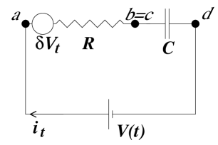
Figure 2: Serial RC circuit with Nyquist noise and imposed voltage.

We note that the behavior of the heat fluctuations in Eq. (7) differs from that of the work fluctuations in Eq. (9) due to exponential tails of the distribution of the heat fluctuationsVanZonCohen03a ; VanZonCohen03b , while those of $P(W_{\tau})$ are Gaussian.

A second example of a circuit that satisfies the extended heat fluctuation theorem is depicted in Fig. 2. Here, the resistor with resistance $R$ and the capacitor with capacitance $C$ are arranged in series and are subject to a linearly increasing voltage source $V(t)=At$. Again, there is a thermal noise generator next to the resistance. The definitions of $i_{t}$ and $q_{t}$ are still that they are the current and charge through $R$ at time $t$, respectively, but $q^{\prime}_{t}=q_{t}$ here, since all charge that runs through $R$ ends up in $C$. We find the appropriate Langevin equation as follows. The imposed voltage, $V(t)$, is equal to the potential difference $V_{ad}=i_{t}R+\delta V_{t}+{q_{t}}/{C}$ (cf. Fig. 2). Using $i_{t}=dq_{t}/dt$ and $V(t)=At$, we find

$$0=-R\frac{dq_{t}}{dt}-\delta V_{t}-\frac{q_{t}-CA\,t}{C}.$$ (11)

This equation is the same as that of Eq. (3) except that $I$ is replaced by $CA$. This means that as far as the current through the resistance is concerned, a constant current source with a capacitor in parallel to it is equivalent to a linearly increasing voltage with a capacitor in series with it. It also means that this case is analogous to the Brownian particle dragged through a fluid by a harmonic potential as well. Quantities for this circuit and the Brownian model can therefore be translated into each other using table 1, except for the work, as we will explain below.

Consider now the heat developed in the resistor during a time $\tau$, which is given by the time integral of the voltage over the resistor, $V_{ab}$, times the current through it, $i_{t}$, so

$$Q_{\tau}=\int_{0}^{\tau}dt\,i_{t}[i_{t}R+\delta V]=-\int_{0}^{\tau}dt\,i_{t}\frac{q_{t}-CAt}{C},$$ (12)

where we used Eq. (11). Note that using $I\sim CA$, this form for $Q_{\tau}$ is the same as in Eq. (5) for the parallel case. Hence, the heat in the serial case behaves precisely the same as in the parallel circuit, because we have seen that $q_{t}$ and $i_{t}$ behave the same in both circuits. Thus, we known that the heat in the serial RC circuit, in the parallel RC circuit and in the Brownian system all behave analogously, and all satisfy the extended FTVanZonCohen03a ; VanZonCohen03b in Eq. (7).

We will now consider the work fluctuations in the serial RC circuit. The work is the time integral of the total current, $i_{t}$, times the total voltage, $V(t)=At$, hence

$$W^{*}_{\tau}=\int_{0}^{\tau}dt\,i_{t}At.$$ (13)

Even when we use $I\sim CA$, this is not the same form as $W_{\tau}$ in Eq. (8) (which is why we added a superscript ^∗), and likewise, using table 1, it is not of the same form as in the Brownian case. Clearly, we cannot use the same results for $W^{*}_{\tau}$ as we obtained for $W_{\tau}$ from the Brownian case or the parallel circuit: we in fact need a additional calculation. For this, we use the method in Ref. VanZonCohen02b . For a Gaussian $P(W_{\tau}^{*})$ one has

$$f^{\mbox{\tiny$W$}*}_{\tau}\equiv\frac{k_{B}T}{\langle W^{*}_{\tau}\rangle}\ln\left[\frac{P(+W^{*}_{\tau})}{P(-W^{*}_{\tau})}\right]=\frac{p_{\mbox{\tiny$W$}}^{*}}{1-\varepsilon(\tau)},$$ (14)

where $p_{\mbox{\tiny$W$}}^{*}=W^{*}_{\tau}/\langle W^{*}_{\tau}\rangle$ and $\varepsilon(\tau)=1-V/(2M)$ with $M=\langle W_{\tau}\rangle$ and $V=\langle(W_{\tau}-\langle W_{\tau}\rangle)^{2}\rangle$. The quantities $M$ and $V$ in turn are calculated using the definition of $W^{*}_{\tau}$ in Eq. (13) and the relations $\langle q_{t}\rangle=CA[t-\tau_{r}(1-e^{-t/\tau_{r}})]$ and $\langle(q_{t}-\langle q_{t}\rangle)(q_{t^{\prime}}-\langle q_{t^{\prime}}\rangle)\rangle=k_{B}TC\,e^{-|t-t^{\prime}|/\tau_{r}}$ (from Ref. VanZonCohen02b , using Table 1). This yields

$$\varepsilon(\tau)=2\frac{\tau_{r}^{2}(1-e^{-\tau/\tau_{r}})-\tau\tau_{r}e^{-\tau/\tau_{r}}}{\tau^{2}}.$$ (15)

Note that this goes to zero asymptotically as $1/\tau^{2}$, which is faster than the $1/\tau$ decay of $\varepsilon(\tau)$ in Eq. (10).

These result so far made no explicit reference to nanoscale circuits. Indeed, these results are valid for a circuit of any size. We will now turn to their relevance for nanocircuits. The extended FT shows that large heat fluctuations are more likely to occur than according to the conventional FT, due to the exponential tails of the distribution of heat fluctuations. This could be important for the design of nanostructures because of the rise of temperature due to heat development. Either the average current through $R$ could be too large or a large heat fluctuation might occur. Fluctuations of the energy exist already in an equilibrium system in contact with a heat reservoir, i.e. a circuit for which $I=0$. In that case, the energy fluctuations of an $N$ atomic resistor will be of the order of $\sqrt{N}k_{B}T$. To explore the properties of nanostructures, composed of just a few atoms, we start with $N=1$. For that case, energy fluctuations are of the order of $k_{B}T$ which, if they were not removed, could amount to a significant increase or decrease of the resistor’s temperature. An estimate of this temperature change can be made using the law of Dulong and Petit that (at room temperatures) the specific heat per atom of a solid is $3k_{B}$. Thus, the change in temperature could be as large as $\Delta T=k_{B}T/(3k_{B})=T/3=100\mathrm{K}$, for $T=300\mathrm{K}$.

In our Langevin theory for the circuits, we have assumed a constant temperature. To still be able to use the theory, we need that the temperature does not vary too much. A similar condition is needed if the resistor is not to fail. To satisfy this condition, the heat developed will have be transported away at a fast enough time scale $\tau_{\mbox{\tiny$T$}}$. If the heat $Q_{\tau_{\mbox{\tiny$T$}}}$ developed in this time is large enough to significantly increase the material’s temperature, failure may occur. The induced temperature difference, given by $\Delta T=Q_{\tau_{\mbox{\tiny$T$}}}/C_{V}$, is insignificant if $\Delta T/T\ll 1$, i.e., if

$$\frac{Q_{\tau_{\mbox{\tiny$T$}}}}{C_{V}T}\ll 1.$$ (16)

This condition should hold both for the average and the fluctuations of $Q_{\tau_{\mbox{\tiny$T$}}}$. Let us first consider the average (i.e., what one would do for macroscopic circuits). In the stationary state of the parallel circuit, the average heat is $Q_{\tau_{\mbox{\tiny$T$}}}=IV\tau_{\mbox{\tiny$T$}}$, where $V=IR$, so

$$\frac{Q_{\tau_{\mbox{\tiny$T$}}}}{C_{V}T}=\frac{I^{2}R\tau_{\mbox{\tiny$T$}}}{C_{V}T}=\frac{\tau_{\mbox{\tiny$T$}}}{\tau_{\mbox{\tiny$H$}}},$$ (17)

where $\tau_{\mbox{\tiny$H$}}={C_{V}T}/{I^{2}R}$. (This in fact also holds for the serial circuit if we replace $I$ by $CA$.) Equation (16) now becomes

$$\tau_{\mbox{\tiny$T$}}\ll\tau_{\mbox{\tiny$H$}}.$$ (18)

That is, the time scale of temperature relaxation given by $\tau_{\mbox{\tiny$T$}}$ has to be fast compared to the heating time $\tau_{\mbox{\tiny$H$}}$. However, even if the average of the heat is well-behaved, the heat fluctuations might still damage the circuit. We need the typical size of these fluctuations. From our previous work on the FTs, we found that for long times $\tau$, $\sqrt{\langle(Q_{\tau}-\langle Q_{\tau}\rangle)^{2}\rangle}\approx\sqrt{2k_{B}T\langle Q_{\tau}\rangle}$VanZonCohen03a ; VanZonCohen03b . Thus, for $\tau=\tau_{\mbox{\tiny$T$}}$, $\sqrt{2k_{B}TI^{2}R\tau_{\mbox{\tiny$T$}}}$ is a typical value for $Q_{\tau_{\mbox{\tiny$T$}}}$ which we can insert into Eq. (16), giving

$$\frac{2k_{B}I^{2}R\tau_{\mbox{\tiny$T$}}}{TC_{V}^{2}}\equiv\frac{\tau_{\mbox{\tiny$T$}}}{\tau_{\mbox{\tiny$F$}}}\ll 1$$ (19)

where the time scale for the heat fluctuations is $\tau_{\mbox{\tiny$F$}}={TC_{V}^{2}}/{2k_{B}I^{2}R}=({C_{V}}/{2k_{B}})\tau_{\mbox{\tiny$H$}}$. For an $N$ atomic solid at room temperature, for which Dulong-Petit is valid, we know that $\tau_{\mbox{\tiny$F$}}/\tau_{\mbox{\tiny$H$}}=C_{V}/2k_{B}$ = $\frac{3}{2}N$. Thus, the factor between $\tau_{\mbox{\tiny$F$}}$ and $\tau_{\mbox{\tiny$H$}}$ is always bigger than one, so that Eq. (19) in fact follows from Eq. (18). As a result, if on average the circuit will not fail, then the fluctuations will not make it fail either. However, for systems below room temperature, for which quantum effects become relevant, the ratio $C_{V}/k_{B}$ can be much smaller than one (i.e. Debye’s law), opening up the possibility that in that case the requirement on $\tau_{\mbox{\tiny$F$}}$ in Eq. (19) could be stricter than that on $\tau_{\mbox{\tiny$H$}}$ in Eq. (18).

Although reassuring, Eq. (19) concerns only typical fluctuations. However, one also needs to be concerned with large fluctuations. Compared to the Gaussian distributed work (or power) fluctuations, large fluctuations for heat are much more likely due to the exponential tails of its distribution function. Furthermore, if the condition in Eq. (16) is not met, temperature variations will occur and the theory then needs to include a coupling to the heat diffusion equation. This could be relevant for future experiments.

In conclusion, we studied work and heat fluctuations in electric circuits using analogies to Brownian systems with non-universal additions to the Nyquist noise-Brownian motion analogy. Our analogy links the work and heat fluctuations in a parallel RC circuit to those in a Brownian system for which the work and heat fluctuations are known to satisfy the conventional FT and extended FT respectively. For the serial circuit, the analogy also works for the heat fluctuations, but not for the work fluctuations. However, a short calculation [below Eq. (13)] shows they still satisfy the conventional FT.

RVZ and EGDC acknowledge the support of the Office of Basic Engineering of the US Department of Energy, under grant No. DE-FG-02-88-ER13847.

References

- (1) D. J. Evans, E. G. D. Cohen, and G. P. Morriss, Phys. Rev. Lett. 71, 2401 (1993); D. J. Evans and D. J. Searles, Phys. Rev. E 50, 1645 (1994).
- (2) G. Gallavotti and E. G. D. Cohen, Phys. Rev. Lett. 74, 2694 (1995); E. G. D. Cohen, Physica A (Amsterdam) 240, 43 (1997); E. G. D. Cohen and G. Gallavotti, J. Stat. Phys. 96, 1343 (1999).
- (3) J. Kurchan, J. Phys. A, Math. Gen. 31, 3719 (1998); J. L. Lebowitz and H. Spohn, J. Stat. Phys. 95, 333 (1999).
- (4) S. Ciliberto and C. Laroche, J. Phys. IV, France 8, Pr6-215 (1998); Recently, another experiment along these lines was done by S. Ciliberto et al. (arXiv:nlin.CD/0311037).
- (5) G. M. Wang et al., Phys. Rev. Lett. 89, 050601 (2002). In this paper, the total work was mistakenly identified with the entropy production.
- (6) R. van Zon and E. G. D. Cohen, Phys. Rev. E 67, 046102 (2003).
- (7) O. Mazonka and C. Jarzynski, Exactly solvable model illustrating far-from-equilibrium predictions, arXiv:cond-mat/9912121.
- (8) R. van Zon and E. G. D. Cohen, Phys. Rev. Lett. 91, 110601 (2003); Non-equilibrium Thermodynamics and Fluctuations, arXiv:cond-mat/0310265 (To appear in Physica A).
- (9) R. van Zon and E. G. D. Cohen, Extended heat-fluctuation theorems for a system with deterministic and stochastic forces, arXiv:cond-mat/0311357 (To appear in Phys. Rev. E).
- (10) See e.g. N. G. van Kampen, Stochastic Processes in Physics and Chemistry (North Holland, Amsterdam, 1992), revised and enlarged ed. and R. M. Mazo, Brownian motion: Fluctuations, Dynamics and Applications (Clarendon Press, Oxford, 2002).
- (11) A self-inductance in series with can result in a mass-like term in Eqs. (3) and (11). To know the status of the FTs for would require an additional calculation.