Breakup of the Hydrogen Bond Network In Water:The Momentum Distribution of the Protons

Abstract

Neutron Compton Scattering measurements presented here of the momentum distribution of hydrogen in water at temperatures slightly below freezing to the supercritical phase show a dramatic change in the distribution as the hydrogen bond network becomes more disordered. Within a single particle interpretation, the proton moves from an essentially harmonic well in ice to a slightly anharmonic well in room temperature water, to a deeply anharmonic potential in the supercritical phase that is best described by a double well potential with a separation of the wells along the bond axis of about .3 Angstroms. Confining the supercritical water in the interstices of a C60 powder enhances this anharmonicity. The changes in the distribution are consistent with gas phase formation at the hydrophobic boundaries.

s PACS numbers, 61.12.Ex, 61.25.Em,82.30.Rs

Although water has been intensively studied with neutron scattering for decades, and much is known about the spatial structure of the various phases of water, Deep Inelastic Neutron Scattering measurements,(or Neutron Compton Scattering) which measure the momentum distribution of the proton, have only become available in the last few years. This distribution, which is determined almost entirely by quantum effects for the systems we have studied, is a sensitive probe of the local environment of the proton, as well as a direct measurement of its dynamics. In crystals, for instance, measurements of the shape of the momentum distribution have been used to extract the Born-Oppenheimer potential for the proton, and its changes with temperature.[1] Here we demonstrate that detailed information can be obtained from powder samples and liquids as well. In particular, we examine the momentum distribution of the protons in water as the regular hydrogen bond network in poly-crystalline ice is disordered, first by melting, then by heating under pressure into the supercritical phase, and then further by embedding the supercritical water in the interstices(typical diameter 100 Angstroms) of a C60 powder. We find that there are in fact dramatic changes, as the momentum distribution responds to changes in the structure of the hydrogen bonded network. The changes upon melting seem well understood, but the results in the supercritical phase are astonishing, as the proton appears to be coherently distributed over two positions along the hydrogen bond separated by about .3 angstroms. The effect of the C60 is consistent with other experiments that show a depleted phase forming at hydrophobic surfaces.

The experiments are done on the electron volt spectrometer, Vesuvio, at ISIS, the pulsed neutron source at the Rutherford Laboratory. This sort of source is needed to provide high energy neutrons(5-100 ev) for which the energy transfer is sufficiently large compared to the characteristic energies of the system that the scattering is given accurately by the impulse[2] approximation limit. The scattering at these energies is entirely incoherent, each particle scattering independently. The scattering cross-section is proportional to $S_{M}(\vec{q},\omega$), the scattering function for a particle of mass M, which is related to the momentum distribution of the particle n($\vec{p}$) in this limit by the relation

$$S_{M}(\vec{q},\omega)=\int n(\vec{p})\delta(\omega-{\hbar q^{2}\over 2M}-{\vec{p}.\vec{q}\over M})d\vec{p}$$ (1)

where $\hbar\omega$ is the energy transfer, M is the mass of the proton, and q=$|\vec{q}|$ is the magnitude of the wave-vector transfer. The probability of observing the proton with momentum $\vec{p}$,$n(\vec{p})$, for simple one particle systems in their ground state, is the square of the absolute value of the Fourier transform of the spatial wave-function. Although there are certainly many body effects in water, the small mass of the proton compared to the surrounding oxygen make this a good first approximation for interpreting the data.[3]

We represent $S_{M}(\vec{q},\omega)$ as ${M\over q}J(\hat{q},y)$ where y=${M\over q}(\omega-{\hbar q^{2}\over 2M})$. The general case, where the momentum distribution results from the proton in a crystal environment, and hence has a 3-D structure, is described in [4]. In the present situation, where the sample is either poly-crystalline or a liquid, the average momentum distribution has no angular dependence, and $J(\hat{q},y)$ is independent of $\hat{q}$.

We will fit the data with a series expansion of the form[5]

$$J(y)={e^{{-y^{2}}\over{2\sigma^{2}}}\over{\sqrt{2\pi}\sigma}}\sum\limits_{n}{a_{n}\over{2^{2n}n!}}H_{2n}({y\over{\sqrt{2}\sigma}})$$ (2)

where the $H_{n}(y)$ are Hermite polynomials.

This series is truncated at some order(2n=14) in this case). The coefficients $a_{n}$ then determine the measured $n(p)$ directly as a series in Laguerre polynomials.

$$n(p)={e^{-}{{p^{2}\over{2\sigma^{2}}}}\over{(\sqrt{2\pi}\sigma)^{3}}}\sum\limits_{n}a_{n}(-1)^{n}L_{n}^{{1\over 2}}({{p^{2}\over{2\sigma^{2}}}})$$ (3)

The procedure is a smoothing operation, which works with noisy data. and which also allows for the inclusion of small corrections to the impulse approximation[4]. The errors in the measured $n(\vec{p})$ are determined by the uncertainty in the the measured coefficients,through their correlation matrix, which is calculated by the fitting program. The coefficient $a_{1}$ is set to zero to avoid redundancy with the variation of $\sigma$. As a consequence, in units in which $\sigma$ is measured in inverse Angstroms, and the energy is expressed in milli-electron volts, the total kinetic energy(for a proton) is K.E.=6.2705$\sigma^{2}$, even for strongly anharmonic momentum distributions . When fit in the way described above, which we will call a free fit,[6] since there is no model assumed, we find that in fact the data can be fit well with two coefficients that are statistically significant, $a_{2}$ and $a_{3}$, and it is these together with $\sigma$ that we present in the Table I below to describe n(p).For more details on the fitting procedure see Ref.[4].

The room temperature water and poly-crystalline ice data were taken in standard aluminum sample holders, 10cm by 10cm by 1mm, thin enough to lead to small multiple scattering which is corrected for in all cases. A cell was designed specifically for the high temperature and high pressure measurements. The background from this ZrTi cell appears as inelastic scattering and is readily subtracted.[4] It can provide pressure up to 2000 bar and temperature up to $450^{o}C$. The sample size in the cell is 7 mm in diameter and 30 mm in height, presenting considerably less sample to the beam than the water and ice measurements, and hence leading to poorer statistics. The heaters and temperature sensors were all inserted in the cell. A 1 mm steel pipe leads to an external water-pressurizer (i.e. a pump) which provided the required pressure. The water used as pressure transfer media and the sample volume was distilled H₂O.

TABLE I.: Parameters for Free Fit

Water Sample	$\sigma(\AA^{-1})$	$a_{4}$	$a_{6}$
Ice -4C	4.579	$.060\pm.0014$	$-.068\pm.016$
Water 23C	4.841	$.185\pm.012$	$.015\pm.015$
T=400C, P=750bar	6.363	$.271\pm.022$	$.157\pm.028$
T=400C, P=750bar in C60	6.439	$.592\pm.054$	$.007\pm.07$

This representation should be regarded as the data for n(p) determined by the measurement. We show in Fig. 1 a comparison of the free fits to the data for ice, water at room temperature, supercritical water, and supercritical water contained in the interstices of a C60 powder. The quantity $4\pi p^{2}n(p)$, the radial momentum distribution is presented, in order to compare quantities with the same normalization. Although the temperature has a profound effect on the structure, for a given structure, it has only a small direct effect on the momentum distribution. The corrections to the momentum widths for the ice due to the excitation of higher vibrational levels is negligible along the bond and only a few percent transverse to the bond. What we are seeing is nearly entirely the ground state momentum distribution, reflecting the average local structure of the proton environment.

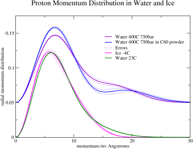
FIG. 1.: Comparison of fits to the data of the radial momentum distribution, 4$\pi p^{2}n(p)$ for a range of conditions from ice to supercritical water in the interstices of a C60 poly-crystalline powder(typical size of pores 100 Å) corresponding to increasing disorder in the hydrogen bond network. The supercritical water data has been displaced upward by .05 for clarity. The density of the supercritical water is .65 gr/cc.

Structural changes in going from ice to water are noticeable in the data. The tail of the distribution is due to the momentum along the bond direction, since the proton is most tightly bound in this direction, and tight binding implies high momentum width. It is clear that this width has increased, which can be interpreted as due to the slight increase in the average hydrogen bond distance in water, so that the proton becomes more tightly bound to its covalently bonded oxygen. The change in the covalent bond length is only 4$\%$, but the measurements are clearly accurate enough to see this shift. This interpretation can also be applied to the supercritical water data. The bonds are expected to be significantly longer or missing altogether explaining the greatly increased momentum width. However, the second peak in that data, is entirely unexpected from a simple picture of the bond. One could try to interpret the second peak as a small population of protons with unusually high momentum. However, this would mean an RMS energy of these protons of approximately 2.5 ev, and a localization length of about .025 Angstroms. We know of no mechanism for producing such energetic protons, and will not consider this possibility further. We will interpret the data in terms of a single particle in an effective potential due to its neighbors. With this interpretation, the second peak indicates that the proton is coherent over two separated sites along the bond. This can be made clear by fitting the data phenomenologically with a model, in which, in a frame of reference where an individual bond is taken to lie along the z axis, the motion transverse to the bond is harmonic and along the bond given by a distribution that corresponds in real space to two Gaussians separated by a distance d. We have then

$$n(p_{x},p_{y},p_{z})={{2cos^{2}({{p_{z}d}\over{2\hbar}})}\over{1+e^{{-2d^{2}\sigma_{z}^{2}}\over{\hbar^{2}}}}}\prod\limits_{i}{e^{-{p_{i}^{2}\over 2\sigma_{i}^{2}}}\over(2\pi\sigma_{i})^{1\over 2}}$$ (4)

We will assume $\sigma_{x}=\sigma_{y}$. We have done fits with this condition relaxed, and find that it is well satisfied. The parameter $\sigma_{z}$ gives the width of the Gaussians in real space through the uncertainty relation. In the case that d=0, we have an anisotropic Gaussian momentum distribution.

This distribution is then averaged over all angles, the corresponding J(y) fit to the data , and the parameters of the model determined.

We show in fig 2 the fits to that model, and in table 1 the parameters obtained for those fits. The ice data is very accurately described by an anisotropic Gaussian. The parameters of the Gaussian correspond to vibrational energies in the transverse and longitudinal directions of 105mev and 332mev respectively.The water data is also well described this way, with a higher stretch frequency of $367$ meV and no change in the transverse frequency, although there are clearly additional anharmonicities that make small corrections that are visible in the figure. These may be due to a variation of the effective potential from site to site in the water, or to an intrinsic anharmonicity in a single bond, perhaps the precursor to the strong anharmonicity seen in the supercritical water data. Indeed, if the distribution were due entirely to a rotationally averaged gaussian, the coefficient of $a_{3}$ would have to be negative, and it is not[7]. Li et al[8] have measured the frequency of vibration for hydrogen impurities in D₂O ice, which should be comparable to the frequencies we infer from the anisotropic harmonic fit to our data. They find that the two transverse vibrations of the proton are at 105 meV and 200 meV, with the stretch mode at 405 meV. The additional contributions to the anharmonic coefficients may be responsible for the discrepancy with Li et al’s results, since the difference in the transverse mode frequencies we obtain by fitting a Gaussian with three different vibrational energies is very sensitive to the value of $a_{3}$.

The fits to the supercritical data require non zero values for the parameter d giving the separation of minima in the potential wells. That is the proton appears to be coherent over sites separated by a distance of approximately .3 angstroms that are both local minima of the potential.

TABLE II.: Parameters for Model Fit

Water Sample	$\sigma_{z}$(Inv. Angstroms)	$\sigma_{x}$(Inv. Angstroms)	d(Angstroms)
Ice -4C	$6.29\pm.51$	$3.53\pm.31$	0
Water 23C	$6.73\pm.08$	$3.51\pm.04$	0
T=400C, P=750bar	$8.40\pm.19$	$5.70\pm.16$	$.316\pm.0045$
T=400C, P=750bar in C60	$9.47\pm.26$	$5.025\pm.11$	$.274\pm.0043$

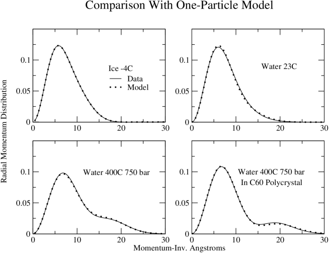
FIG. 2.: Comparison of radial momentum distribution, 4$\pi p^{2}n(p)$ with a one-particle model based on double wells along the bond direction, Eq. 4 . The additional peaks in the supercritical water data are due to coherence over wells separated by distances of the order of .3 Angstroms in this model. There is only one well for the room temperature water and the ice data.

We know of no prediction of such an effect. The disorder in the hydrogen bond network would lead to bifurcated bonds, bent bonds double bonds and missing bonds. It would seem that these would lead to tunnelling motions transverse to the bond. In our experiment, however, the tunnelling, or more precisely, the coherence, shows up along the axis with a high momentum width, which is surely the axis of stretching of the covalent bond. To the extent that there are linear bonds, this would be the bond axis. In fact, it is reasonable to think that the supercritical water is made up of small clusters that combine and break up on a time scale much longer than our observation time, so we are seeing a snapshot average of the ground states for the proton in these small clusters.[9] It is possible then, that what we are seeing is the effect of cooperative tunnelling between single bonds through the intermediate state of a bifurcated bond , as observed in trimers and small clusters [10]. Although the cooperative tunneling motion in these small clusters involves primarily the transverse motion, this could be accompanied, due to a coupling of the longitudinal and transverse modes, by changes in the momentum distribution along the bond direction, which is what we see. We note in this regard that the interpretation in terms of a single particle effective potential, although it fits well, is only a phenomenological representation of a more complex many-body phenomenon. We also note that a double well potential has been posited as an explanation for the extroardinarily large Debye-Waller factors observed in water in the interior of carbon nanotubes,[11] suggesting that it is the disorder of the network that is the origin of the double well potential there too.

The wells are sufficiently separated that the wave-function actually becomes bimodal. We show in fig 3 the probability, (the wave-function squared) corresponding to the fitted momentum distributions for three of the measurements, together with the potential that would produce that wavefunction.

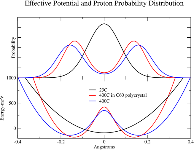
FIG. 3.: Comparison of probability, based on an effective single particle model, for finding a proton at a position along the bond. The zero position is unknown from our experiments, so that the coordinate is relative to the most probable position. The ice and room temperature results are Gaussian, corresponding to harmonic wells. The high temperature wavefunctions are assumed to be the sum of two Gaussians separated by some distance(Table II), and the potential is that which would produce those wavefunctions.

One can expect that the the hydrogen bond network will be even more distorted for the water in the interstices of the powdered C60 than in the pure water, and we will be seeing an average over bonds that are near the surface with those that are relatively ”in the bulk”. The size of the surface layer at ordinary temperatures is in some dispute[12, 13], ranging from 1.5-5nm and it seems certain that it would be significantly larger for the supercritical water. It is conceivable, given the size of the interstices in the C60 poly-crystal, that the entire volume of water would be strongly affected by the contact with the surfaces. Consistent with this, we find that the protons are more localized in the C60 interstices than in the ”free” supercritical water.

In conclusion, the results shown here, in addition to providing a detailed picture of the dynamics of the proton in water, show that the momentum distribution of the proton can be measured with sufficient accuracy to provide detailed information about the local structure, even in liquids or powder samples.

REFERENCES

- [1] G. Reiter, J. Mayers , P. Platzman, Phys. Rev. Letts. 89, 135505 (2003)
- [2] P. M. Platzmann, in Momentum Distributions, ed R. N. Silver and P. E. Sokol (Plenum Press,New York, 1989, p249)
- [3] M. Warner, S. W. Lovesey, , and J. Smith, Z. Phys. B 39, 2022 (1989)
- [4] G. Reiter, J. Mayers, and J. Noreland, Phys. Rev. B,65, 104305, (2002)
- [5] This is equivalent to the usual representation by virtue of the identity in M. Abramowitz and I. Stegun, National Bureau of Standards Applied Mathematics Series 55, 1964 P779
- [6] D. Sivia,’Data Analysis:A Bayesian Tutorial’,Clarendon Press, Oxford (1996)
- [7] The average may be done analytically. For the case that the two transverse directions have the same variance, we find is of the form given in Eq.2, with , , and = , where . Explicitly, = and
- [8] J.C.Li et al, J. Chem. Phys. 105, 6733, (2003)
- [9] M. Boero et al, Phys. Rev. Letts. 85, 3245, (2000)
- [10] F.N.Keutsch and R. J. Saykally, Proc. Nat. Acad. Sci. 98,10533,(2001)
- [11] A.I. Kolesnikov et al, (to be published)
- [12] T.R. Jensen et al, Phys. Rev. Letts. 90, o86101, (2003)
- [13] R. Steitz et al, Langmuir, 19, 2409, (2003)
- [14] C.H.Uffindell et al, Phys.Rev.B 62, 5492,(2000)