Can One Make Any Crash Prediction in Finance Using the Local Hurst Exponent Idea?

Abstract

We apply the Hurst exponent idea for investigation of DJIA index time-series data. The behavior of the local Hurst exponent prior to drastic changes in financial series signal is analyzed. The optimal length of the time-window over which this exponent can be calculated in order to make some meaningful predictions is discussed. Our prediction hypothesis is verified with examples of ’29 and ’87 crashes, as well as with more recent phenomena in stock market from the period 1995-2003. Some interesting agreements are found.

1 Introduction

Financial markets are nonlinear, complex and open dynamical systems described by enormous number of free, mostly unknown parameters. Many of these parameters are exterior for the market, what makes the full description of the system even more complicated. Exterior parameters are completely out of control by investors who are the part of financial system. These parameters have usually random origin connected with e.g. political disturbances, terrorist attacks, bankruptcies of leading companies, wars, etc. There are also investor dependent interior parameters driving the market even in the absence of other, not expected exterior phenomena. The full recognition of such interior parameters is a big challenge for economists and econophysicists.
All these circumstances mean that detailed time evolution of a complex financial system is unpredicted. However is the situation so hopeless? Even if we can not predict the detailed evolution scenario, we might be able to say something else about the system. We have learned from statistical mechanics that one does not have to know where a particular particle of the mechanical system will be a second or few from now, in order to find equation of state of this system. The latter is quite sufficient in practical applications giving us the whole available information about the macroscopic parameters, like e.g. pressure or temperature, and it reflects all detailed microscopic, directly inaccessible information. In many cases this knowledge is sufficient to indicate direction in which the system is evolving.
In this article we rise the question if it is possible to find some macroscopic parameters in financial market which would play the role of a macroscopic indicator of complex, interior stock dynamics. In particular, we would like this parameter to be able to predict that crashes or other drastic changes in the market signal are coming soon. The task looks hopeless if one assumes following Fama [1] that investors destroy information while using it, so that others can not use this information again. In this spirit market should not exhibit any correlations between returns $r_{t}$ at time $t$ and $r_{t+\tau}$ at time $t+\tau$, where

$$r_{t}=\ln{\frac{S_{t+1}}{S_{t}}}$$ (1)

and $S_{t}$ is the price of a given stock at time $t$.
It was widely believed for a long time that price changes follow an independent, zero mean, Gaussian process. However, deviations from this simple scenario have been observed in the financial signal in the last few years. Empirical work showed that the distribution function $P_{r}(r>x)$ has tails obeying power law relation $P_{r}(r>x)\sim x^{-\alpha}$ [2-4], contrary to normal Gaussian distribution. Also the autocorrelation function of the absolute value of price changes shows long-range persistence $\langle|r_{t}||r_{t+\tau}|\rangle\sim\tau^{-\mu}$, with $\mu\approx 0.3$ [5-7]. A sort of long memory correlations in financial signal itself has also been revealed [8-12].
Due to large liquidity of currency exchange markets, they seem to be a natural subject to explore the existence of such correlations between returns. This has been done for major world and European currencies in [13-15]. It has also been proven that complexity of a financial market is not limited to the statistical behavior of each financial time series forming it but follows from the statics and dynamics of correlations existing between various stocks in the market [16].
The proven existence of correlations in financial time series reveals the possibility to apply some global macroscopic approach to see them. In this paper we address the possibility of searching for correlations between subsequent returns in financial series with the use of Detrended Fluctuation Analysis (DFA)[17], applied for the first time in finances in [18-20]. Our philosophy is described below.

2 The Search for the Market State with the Use of Local Hurst Exponent

It is well known that the Hurst $\alpha$-exponent [21,22], extracted from the time series according to DFA method, measures the level of persistency in the given signal. The value $\alpha\neq 1/2$ implies the existence of long-range correlations and corresponds to so called fractional Brownian motion [23]. In particular, for $\alpha>1/2$ there is persistence, and for $\alpha<1/2$ ’antipersistence’ in the series signal. We expect that dramatic changes in financial signal should be preceded by excitation state of the market (nervousness), what in turn is reflected by the shape of subsequent daily changes in the signal. These changes should become less correlated just before the dramatic breakdown in the signal trend. Contrary, when the trend in the market is strong and well determined, an increasing (decreasing) value of market index in immediate past makes also an increasing (decreasing) signal in the immediate future more probable [24]. In other words, one should observe some long-range correlations in returns and consequently higher $\alpha$ values for strong, long lasting trends (increasing or decreasing ones), and significant drop in $\alpha$-exponent value if the trend is going to change dramatically its direction in very near future.
To check this hypothesis we used DFA technique, rather than other available methods like spectral analysis or rescaled range analysis, to extract $\alpha$-exponent. This is because DFA method avoids detection of long-range correlations being an artefact of nonstationarity of time series [25]. Then some applications were performed for Dow Jones Industrial Average (DJIA) daily closure signal.
For completeness let us briefly remind the main steps of DFA analysis:

1. The time series of random one variable sequence $x(t)$ of length $N$ is divided into $N/\tau$ non-overlapping boxes of equal size $\tau$. The time variable is discrete and evolves by a single unit between $t=1$ ($x(t=1)\equiv x_{1}$) and $t=N$ $(x(t=N)\equiv x_{N})$. Thus each box contains $\tau$ points and $N/\tau$ is integer.

2. The linear approximation of the trend in each $\tau$-size box is found as $y_{\tau}(t)=a_{\tau}t+b_{\tau}$, with $a_{\tau},b_{\tau}$ some box dependent constants.

3. In each $\tau$-size box one defines the ’detrended walk’ $x_{\tau}(t)=x(t)-y_{\tau}(t)$ as the difference between the original series $x(t)$ and the local trend $y_{\tau}(t)$.

4. One calculates the variance about the detrended walk for each box:

   $$F^{2}_{i}(\tau)=\frac{1}{\tau}\sum\limits_{t\in i-th\,box}(x(t)-y_{\tau}(t))^{2}\equiv\frac{1}{\tau}\sum\limits_{t\in i-th\,box}x_{\tau}^{2}(t)$$ (2)

   and the average of these variances over all $N/\tau$ boxes of size $\tau$:

   $$\langle F^{2}(\tau)\rangle=\frac{\tau}{N}\sum\limits^{N/\tau}_{i=1}F^{2}_{i}(\tau)$$ (3)

5. A power law behavior is expected:

   $$\langle F^{2}(\tau)\rangle\sim\tau^{2\alpha}$$ (4)

   from which $\alpha$-exponent can be extracted from log-log linear fit.

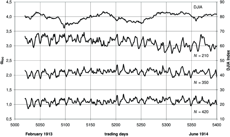
Figure 1: The example of time evolution plots of local $\alpha$-exponent for DJIA signal in the period Feb.1913–June 1914 for three different choices of time-window length $N$: $N=210$, $350$, $420$. The $\alpha$ values are artificially multiplied by two and then displaced along the vertical axis to make the differences noticeable. The DJIA index signal is also drawn for comparison.

If one wants to use $\alpha$-exponent to measure the strength of local correlations in financial time series, one has to use the local $\alpha$-exponent idea [17, 18]. For a given trading day $t=i$, the corresponding $\alpha_{i}$-exponent value will be calculated according to Eq.(4) in the period $\langle i-N+1,i\rangle$ of length $N$, called an observation box or time-window. In order to cover the whole time-window length $N$ with $\tau$-size boxes, we put the last box contributing to Eq. (3) in the period $\langle i-N+1,i-[\frac{N}{\tau}]\tau+1\rangle$, where $[.]$ means the integer part. This box partly overlaps the preceding one but such overlapping does not modify the local $\alpha$. Moving the time-window every one session, one is able to reproduce the history of $\alpha$ changes in time. Let us notice that only the past signal of financial series, not earlier than $N$ sessions before a given trading day $t$, contributes to local $\alpha$ value.
It is not surprising that local $\alpha$-exponent at given moment $t$ depends on the time-window length $N$. It is seen in Fig.1 where we present the example of local $\alpha$-exponent plots for chosen $400$ trading day period of DJIA daily closure values. Three different choices: $N=210$, $N=350$ and $N=420$ have been here made to calculate local $\alpha$. One may notice that plots for $N=350$ and $N=420$ coincides very well with each other, while $N=210$ plot shows already some deviations from other two. It exhibits slightly higher local $\alpha$ values in the first half of discussed period than in the second half. The question arises, whether this is a real effect outside the statistical uncertainties range and what the optimal time-window length $N$ should be chosen for further discussion.
The choice of $N$ seems to be a matter of intuition, statistics and economic regards. If $N$ is too large, $\alpha$-exponent loses its locality and may not ’see’ correlations whose characteristic range, say $\rho$, is much smaller than the window length ($\rho\ll N$). This is the main reason why $\alpha$ evolution becomes more smooth if $N$ increases. On the other hand, it has been proven that standard deviation $\Delta\alpha$ in the local $\alpha$ value, caused by finite-size time-series effects on long-range correlation, is of order [26]:

$$\Delta\alpha\sim(\frac{\tau}{N})^{1/2}$$ (5)

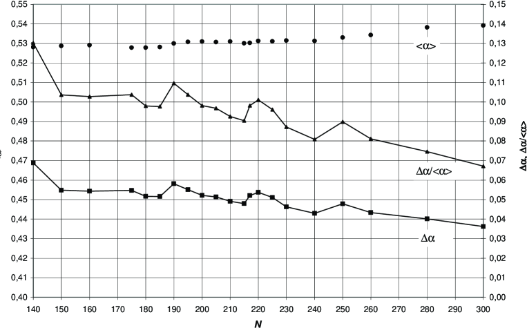
Figure 2: The standard deviation $\Delta\alpha(N)$ and the percentage uncertainty $\Delta\alpha/\langle\alpha\rangle$ with respect to the mean $\alpha$ value $\langle\alpha\rangle$ as a function of time-window length $N$. Calculations were made on the sample of $500$ subseries of length $N$ each. Note that $\langle\alpha\rangle$, marked with round dots, stays steady and does not change significantly with $N$. It confirms the right choice of subseries in DJIA signal. Such subseries with uncorrelated signal and no drastic changes in $\alpha$-exponent (quiet domains) are good, natural tools to calibrate statistical uncertainties of the applied method.

Thus, we are stuck with huge statistical uncertainty with decreasing $N$, what efficiently destroys all predictions.
One has to find then a golden point (golden area) where two above requirements meet together, i.e. where $\Delta\alpha$ is sufficiently small, and $N$ is not too large. For economic reason we suggest that $N$ should not exceed one trading year ($N=240$) in the case of financial series with daily closure signal. This is to avoid probable seasonal periodicity in supply and demand in the market, what would introduce artificial contributions to investigated correlations. Besides, in our opinion, $\alpha$ loses a sens of the local value for $N>240$. In order to stay within the scaling range of Eq. (4) we used the box size $5<\tau<N/5$.
To find the optimal $N$ we investigated how far the standard deviation $\Delta\alpha$ changes with $N$ for $N\leq 300$. This has been done for different subseries of DJIA signal, taking $500$ samples for each value of $N$. The results are collected in Fig. 2, where $\Delta\alpha(N)$ is displayed together with the respective percentage uncertainty $\Delta\alpha/\langle\alpha\rangle$. As one would expect from Eq. (5), $\Delta\alpha(N)$ slowly decreases on the average with $N$, but some departs from this rule are observed. The first local minimum below $N=240$ appears at $N=215$. Although this minimum is not strong, we decided to make further estimations of local $\alpha$ for DJIA series using this particular time-window length. Our choice corresponds to about ten months trading period. It is worth to observe that the obtained statistical uncertainty $\sim 9\%$ agrees well with that calculated in [18] for a monetary market. We have also checked that, for $N<200$, there exists a substantial drop of linear regression correlation coefficient $R^{2}$, what additionally justifies our choice. Finally, we found that the local $\alpha$ value is not sensitive to changes in $N$ not exceeding $10\%$, so that any choice $190\leq N\leq 230$ reproduces qualitatively and quantitatively very similar results.

3 DJIA Signal Tested with DFA Method - Applications

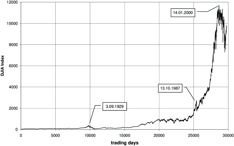
Figure 3: The whole daily closure DJIA index history (1896-2003). The major economic events are seen as clear local maxima. They are marked with arrows indicating also the date of economic event.

Now we proceed to analyze the local value of $\alpha$-exponent estimated with the DFA technique for daily closure DJIA signal. The whole history of this signal is collected in Fig.3. We have focused attention on the most important events in the market history. These are: crashes in September 1929, October 1987, July 1998, and the current situation in last three years. All data were taken from [27].
First let us consider the ’29 crash shown in details in Fig.4. The DJIA signal had been in clear increasing mode for about $4$ months - from session $\sharp 9760$ up to the session $\sharp 9840$ (3.09.1929) when the trend in market index changed its direction. The crash took place 40 days later. The detailed $\alpha$-exponent structure of this period is shown in Fig.4a, where dots denote respective local $\alpha$ values calculated session by session from the last $N=215$ index values. To see more effectively the evolution of local $\alpha$, the moving average value $\alpha_{m5}$ of $\alpha$-exponent taken from five last sessions (one trading week) has been drawn in Fig.4b. A very clear decreasing trend in local $\alpha$ is visible. It had started about one month before the DJIA index reached its maximal value on 3.09.1929, but did not terminate with this date. Small corrections in local $\alpha$ around the session $\sharp 9840$ can be explained as a result of change in DJIA index trend at that time. The $\alpha$-exponent has reached a deep and clearly seen local minimum $\alpha\sim 0.45$ two weeks before the crash, contrary to very high value $\alpha\sim 0.65$ from which it started several months earlier. The statistical uncertainty in the difference between initial ($\alpha_{0}$) and final ($\alpha_{f}$) values is at most $(\Delta\alpha_{0}/\alpha_{0}+\Delta\alpha_{f}/\alpha_{f})\sim 18\%$ - twice smaller than the respective change $(\alpha_{f}-\alpha_{0})/\alpha_{0}\sim 33\%$. Hence, statistics is unable to explain this particular trend-like pattern in $\alpha$-exponent values.
To see if it was a chance, we checked two other major crashes in American market in 1987 and 1998. The scenario found for them is revealed in Fig.5 and Fig.6. The ’87 crash has also clear decreasing trend in local $\alpha$ for the whole one year period preceding the crash point (see details in Fig.5). At the same time, DJIA signal constantly rises. These two contradicting trends suggest that investors were becoming gradually more sceptic about the market future at that time, despite the market index has been rising.
The local $\alpha$ had started to reach the value below $0.45$ since the session $\sharp 25340$. Soon after, the DJIA index also changed drastically its trend on 25.08.87 (session $\sharp 25385$). A comparison of $\alpha$ increase later on, with simultaneous drop in DJIA signal between sessions $\sharp 25385$ and $\sharp 25395$, can be read as the confirmation of decreasing trend in the market. It is worth to observe that the local $\alpha$ gains again even deeper minimum $\alpha\simeq 0.43$ just before the October crash. This minimum reveals again that the market is very ’nervous’ and that the increase of DJIA index, initiated by session $\sharp 25403$, is only a small correction before the forthcoming crash. The percentage drop between maximal and minimal $\alpha$ value in the trend is about the same as in ’29 crash.
The same phenomena occurs for ’98 crash if we make its ’X-ray’ with the use of local $\alpha$-exponent as seen in Fig.6. The market is much more nervous at that time (the DJIA index plot is jagged much more than ever before). This leads to much smaller values gained by $\alpha$ in its decreasing trend before the crash.
In this particular case it is interesting to see what happened next, i.e. after July 1998. The DJIA index run in the period 1995-2003 is displayed in Fig.7. We notice that just after the ’98 crash, market entered into globally increasing, but very nervous trend lasting up to January 2000. The $\alpha$-exponent increases in this period, however, it probably gets many noise signals coming from the frequently changing DJIA index value within $N=215$ time-window length from the immediate past. In other words the correlation range is too short with respect to $N$ and $\alpha$-exponent loses its sensitivity to detect them. Therefore the prediction of market signal evolution with the use of local $\alpha$-exponent becomes difficult in the period 1995-2003.

4 Conclusions

We think that the careful analysis of local $\alpha$-exponent signal may significantly help to determine in which mode (strong increasing, decreasing or unpredicted one) a market is at given moment. As we have shown, the collected data suggest that very clear trends can be distinguished not only for the financial series signal but also for the local Hurst exponent. In particular, we tested that $\alpha$ value drops significantly before any crash in the DJIA signal is going to happen. This confirms that local Hurst exponent may be used as a measure of actual excitation state of the market. However, one has to remember that strong, exterior phenomena not controlled by investors are able to decelerate or accelerate predicted process, drastically change its depth, or even its direction. Such sudden exterior phenomena can not, of course, be predicted by the local $\alpha$ behavior.
The best results in prediction of forthcoming drastic changes in the market seem to be obtained if ’quiet’ situation exists within considered time-window length, i.e. if one has clear long-lasting trends in market index before the crash. This situation took place in 1929, 1987 and 1998. Otherwise, the $\alpha$-exponent contains artifacts from the rapidly changing market index within time-window over which it is calculated. In the latter case predictions are troublesome.
We have checked that the above analysis, based on the local $\alpha$-exponent, works well also for other market indices, like the Warsaw Stock Exchange Index (WIG 20) [28], however different time-window length should be used in that case. We believe that observation and analysis of local Hurst exponent may play a significant role as an additional hint for market investors, apart from other technical indicators like moving average or momentum. It could be a novel part of the classical technical analysis in finances.

Acknowledgements

One of the autor (D.G) would like to thank M. Ausloos for helpful comments and discussion while this article was in preparation.

Figure 4: An ’X-ray’ of the ’29 crash made with the use of local $\alpha$-exponent.
(a) All local $\alpha$ values calculated session after session are marked as dots.
(b) The moving average $\alpha_{m5}$ of last five sessions. The significant drop in $\alpha$ between sessions $\sharp 9820$ and $\sharp 9860$ is striking.

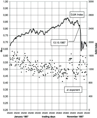
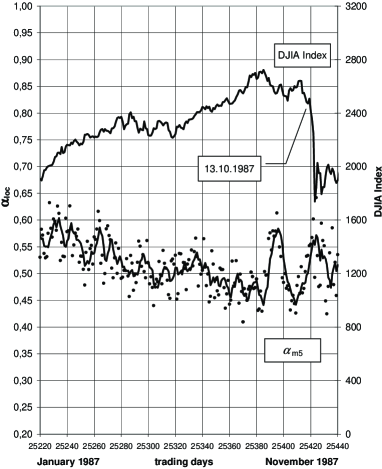
Figure 5: The history of ’87 crash.
(a) The local $\alpha$ evolution calculated as before for $N=215$.
(b) The moving average $\alpha_{m5}$ line explains how the decreasing trend in $\alpha$ is formed.

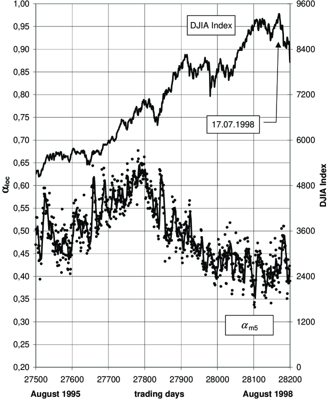
Figure 6: The history of ’98 crash. The same notation as previously applies.
The decreasing trend in $\alpha$ is much deeper ($50\%$) than before. The investors seem to be very enthusiastic till the beginning of 1997 ($\alpha>0.65$), but they become pessimistic and nervous just one year later ($\alpha<0.45$), despite the DJIA index still grows. The $\alpha$-exponent reaches its deep minimum ($\alpha<0.35$) in the half of 1998. This is a good moment for crash to appear(!).

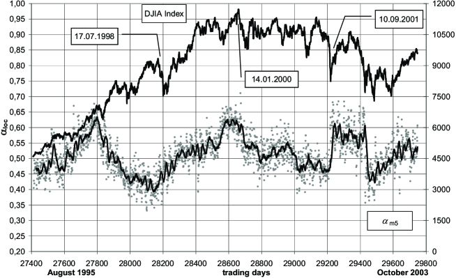
Figure 7: The total display of the period 1995-2003 in DJIA signal history. The previous notation applies. Some important events are marked: the beginning of ’98 crash (17.07.1998), the end of the longest economic boom in US history after $107$ months of its expansion (14.01.2000), terrorist attack in New York (11.09.2001). The decreasing trend in $\alpha$-exponent is observed from 14.01.2000 to 10.09.2001 – just one day before the terrorist attack. The huge drop in DJIA signal was then predicted at that time anyway (!). The DJIA index would have dropped immediately after, even if the attack did not take place (!).

References

- [1] E.F. Fama, J. Finance 25, 383 (1970).
- [2] T. Lux, Appl. Financial Econom. 6 (1996) 463-475.
- [3] V. Plerou, P. Gopikrishnau, L.A.N. Amaral, M. Meyer, H.E. Stanley, Phys. Rev. E 60 (1999) 6519-6529.
- [4] U.A. Muller, M.M. Dacorogna, O.V. Pictet in: R.J. Adler, R.E. Feldman, M.S. Taqqu (Eds.), A Practical Guide to Heavy Tails, Birkha̋user, Basel, 1998, pp. 83-311.
- [5] C.W.J. Granger, Z. Ding, J. Econometrics 73 (1996) 61.
- [6] Y. Liu, R. Gopikrishnan, P. Cizeau, M. Meyer, C.-K. Peng, H.E. Stanley, Phys. Rev. E 60 (1999) 1390-1400.
- [7] M. Lundin, M.M. Dacorogna, U.A. Muller, Financial Markets Tick by Tick, Wiley, New York, 1999, p.91.
- [8] Z. Ding, C.W.J. Granger, R.F. Engle, J. Emp. Finance 1, 83 (1993).
- [9] R.T. Baillie, T. Bollerslev, J. Int. Money & Finance 13, 565 (1994).
- [10] P. De Lima, N. Crato, Economic Lett. 45, 281‘(1994).
- [11] A. Pagan, J. Emp. Finance 3, (1996) 15.
- [12] R.T. Baillie, J. Econometrics 73, (1996) 5.
- [13] M. Ausloos, K. Ivanova, Int. J. Mod. Phys. C 12, (2001) 169.
- [14] K. Ivanova, M. Ausloos, Eur. Phys. J. B 27, 239-247 (2002).
- [15] R. Baviera, M. Pasquini, M. Serva, D. Vergni, A. Vulpiani, Eur. Phys. J. B 20, 473-479 (2001).
- [16] F. Lillo, R.N. Mantegna, arXiv: cond-mat/0006065.
- [17] C.-K. Peng, S.V. Buldyrev, S. Havlin, M. Simons, H.E. Stanley, A.L. Goldgerger, Phys. Rev. E 49 (1994) 1691-1695.
- [18] N. Vandewalle, M. Ausloos, Physica A 246, (1997) 454-459.
- [19] M. Ausloos, N. Vandewalle, Ph. Boveroux, A. Minguet, K. Ivanova, Physica A 274 (1999) 229-240.
- [20] N. Vandewalle, M. Ausloos, Int. J. Comput. Anticipat. Syst. 1 (1998) 342-349.
- [21] H.E. Stanley, S.V. Buldyrev, A.L. Goldberger, S. Havlin, C.-K. Peng, M. Simmons, Physica A 200 (1996) 4-24.
- [22] S.V. Buldyrev, N.V. Dokholyan, A.L. Goldberger, S. Havlin, C.-K. Peng, H.E. Stanley, G.M. Viswanathan, Physica A 249 (1998) 430-438.
- [23] B.B.Mandelbrot, The Fractal Geometry of Nature, W.H.Freeman, New York, 1982
- [24] M. Ausloos, K. Ivanova, arXiv: cond-mat/0108013.
- [25] H.E. Stanley, L.A.N. Amaral, S.V. Buldyrev, A.L. Goldberger, S. Havlin, H. Leschhorn, P. Maass, H.A. Makse, C.-K. Peng, M.A. Salinger, M.H.R. Stanley, G.M. Viswanathan, Physica A 231 (1996) 20-48.
- [26] C.-K.Peng, S.V.Buldyrev, A.L.Goldberger, S.Havlin, M.Simons, H.E.Stanley, Phys.Rev. E 47 (1993) 3730-3733
- [27] http://www.djindexes.com
- [28] D.Grech, Z.Mazur, unpublished