Bulk inhomogeneous phases of anisotropic particles: A fundamental measure functional study of the restricted orientations model

Abstract

The phase diagram of prolate and oblate particles in the restricted orientations approximation (Zwanzig model) is calculated. Transitions to different inhomogeneous phases (smectic, columnar, oriented, or plastic solid) are studied through minimization of the fundamental measure functional (FMF) of hard parallelepipeds. The study of parallel hard cubes (PHC’s) as a particular case is also included motivated by recent simulations of this system. As a result a rich phase behavior is obtained which include, apart from the usual liquid crystal phases, a very peculiar phase (called here discotic smectic) which was already found in the only existing simulation of the model, and which turns out to be stable because of the restrictions imposed on the orientations. The phase diagram is compared at a qualitative level with simulation results of other anisotropic particle systems.

I Introduction

Onsager first showed that the isotropic-nematic liquid crystal phase transition occurs in systems of anisotropic particles interacting via hard core repulsions Onsager . He studied a system of hard spherocylinders in the limit of infinite anisometry $\kappa=(L+D)/D\to\infty$ ($\kappa$ is the spherocylinder length to breath ratio) using the second virial form of the free energy, which in this limit is exact for the isotropic phase. The effect that higher virial coefficients have in the isotropic-nematic transition was later studied by Zwanzig, who introduced a model of hard prolate uniaxial parallelepipeds with axes oriented along the three perpendicular directions Zwanzig . This peculiar model, which obviously treats the orientational degrees of freedom in an unrealistic way, has the advantage of being accessible to the calculation of higher virial coefficients up to seventh order in the infinite aspect ratio limit. He showed that including all these virials the isotropic-nematic transition also occur, although the exact value of the coexisting nematic density strongly depends on the order of the approximation. The Padé approximant generated by the truncated cluster expansion provides a much more stable sequence of the parameters which characterize the transition Runnels . This stability leaves little room for doubts regarding the existence of the transition in the model. The virial expansion resumed and expressed in the variable $y=\rho/(1-\rho v)$, with $\rho$ the number density of parallelepipeds and $v$ their volume, converges more rapidly than the traditional expansion in $\rho$, as was shown by Barboy and Gelbart for different hard particle geometries Barboy . Thus, the so-called $y_{3}$ expansion of the Zwanzig model was applied to the study of the isotropic-nematic transition as well as to the study of properties of its interface Moore . For the latter the authors applied the smoothed density approximation of the free energy functional in the spirit of Tarazona’s weighted density approximation for the fluid of hard spheres Tarazona .

The restricted orientations model for hard cylinders was also used to describe the structural properties of molecular fluids near hard walls or confined in a slit. This time the density functional was constructed from the bulk direct correlation function approximated by a linear combination of geometrical functions Rickayzen .

Computer simulations of a variety of models of nonspherical hard core particles showed that the excluded volume effects could not only account for the stability of nematics, but also for the existence of liquid crystal inhomogeneous phases such as the smectic Strobants_1 and columnar Veerman phases. Particularly the complete phase diagram of freely rotating hard spherocylinders Bolhuis , including not only smectic, but also a plastic solid phase and different oriented solid phases was calculated. Several density functional theories, all of them based on weighted or modified weighted density approximations, are able to reproduce reasonably well the isotropic-smectic or nematic-smectic transitions Somoza ; Poniewierski ; Velasco in the whole range of aspect ratios where the smectic is stable, and in some cases, transitions from the isotropic fluid to the plastic or oriented solid phases Graf . In all these approximations the excess free energy is evaluated by integration of the free energy per particle of a reference fluid (typically spheres or hard parallel ellipsoids) evaluated at some weighted or effective density. In some cases, the employed weight is directly the normalized Mayer function between spherocylinders Poniewierski ; Velasco ; in others, it is calculated from the knowledge of the bulk correlation function of the reference fluid Velasco . For the latter case, the term proportional to the Mayer function enters into the integrand as a multiplicative factor of the free energy per particle. The hard sphere free energy functional is recovered in both approaches as the limiting case of $L=0$.

The fundamental measure theory (FMT) first developed for hard spheres by Rosenfeld Rosenfeld_1 was another starting point for constructing a density functional for anisotropic particles. In its general formalism the excess free energy density of the fluid is a function of some weighted densities obtained by convoluting the density profiles with weights which are characteristic functions of the geometry of a single particle whose integrals are the so-called fundamental measures: volume, surface area, and mean radius of the particles. Unfortunately, the Mayer function of two convex anisotropic bodies cannot be decomposed as a finite sum of convolutions of single particle weights Rosenfeld_2 , which is the keystone for constructing such a functional. Thus, the low density limit of the direct correlation function is no more the Mayer function.

In spite of this, Chamoux and Perera have taken advantage of Rosenfeld’s extension of FMT to hard convex bodies by using it to compute the direct correlation function and patching out the low density limit with the exact Mayer function Chamoux_1 . In this way they have obtained the equation of state for various convex hard bodies (such as hard ellipsoids, spherocylinders, and cut spheres), have predicted ordered phases and, recently, have study demixing in binary mixtures of rigidly ordered particles Chamoux_1 ; Chamoux_2 .

Following a similar procedure a density functional for anisotropic particles has been proposed which interpolates between the Rosenfeld’s hard sphere functional and Onsager’s functional for elongated rods. The resulting model was tested by calculating the isotropic-nematic transition in systems of hard spherocylinders and hard ellipsoids Cinacchi .

Although the authors of this work suggest that the resulting theory can be applied to the study of inhomogeneous systems, the huge computational efforts that their numerical implementations involve is the reason for the absence of any result in this direction. One way to circumvent this difficulty is to reduce the continuous orientational degree of freedom to three discrete orientations (Zwanzig model). Implementing this idea some authors have recently applied the Zwanzig model to the study of interfacial properties of the hard rod fluid interacting with a hard wall or confined in a slit, for a one-component vanRoij and a polydisperse mixture Martinez-Raton_1 , and also to the study of bulk and interfacial properties of hard platelet binary mixtures Harnau . All these models are based on Onsager’s density functional approximation. The increase of the number of allowed orientations in this functional particularized for hard spherocylinders results in the presence of an artificial nematic-nematic transition in the one component fluid as the authors of Ref. vanRoij_1 have shown. This result indicates that certain cares must be taken in the direct extrapolation of the results obtained from this theory.

FMF was also constructed for a mixture of parallel hard cubes combining Rosenfeld’s original ideas with a dimensional cross over constraint Cuesta . The latter appears to be very important to describe correctly the structure of inhomogeneous fluids in situations of high confinement and to describe well the structural properties of the solid phase Tarazona_1 . The dimensional cross over has been used as an important ingredient to develop a density functional for a binary mixture of hard spheres and needles, assuming that the needles are too thin to interact with each other directly Schmidt .

Taking a ternary mixture of parallel hard cubes and scaling each species along one of the three Cartesian axes with the same scaling factor a FMF for the Zwanzig model is obtained. This functional has already been applied to the study of the effect that polydispersity has on the stability of the biaxial phase in a binary mixture of rods and plates Martinez-Raton_2 and on the relative stability of the smectic and columnar phases due to the presence of polydispersity Martinez-Raton_3 .

The FMF for Zwanzig’s model in the homogeneous limit coincide with the scaled particle theory and thus with the so-called $y_{3}$ expansion which, as pointed out before, first began to be used in Ref. Moore as a model to study the isotropic-nematic phase transitions in fluids of hard parallelepipeds. But this functional, through its minimization, also allows us to calculate inhomogeneous density profiles. This functional has been applied recently to study the isotropic-nematic interface of a binary mixture of hard platelets Bier . Its structural and thermodynamic properties resulting from the FMF minimization show complete wetting by a second nematic. The same phenomenon was found in a binary mixture of hard spherocylinders Shundyak .

The phase diagram for Zwanzig’s model including the smectic, columnar, and solid phases has never been carried out, only spinodal instability boundaries have been traced Martinez-Raton_3 . The main purpose of this work is to obtain the complete phase diagram for this model and to compare the results with the only existing simulation of the lattice version of the model, which has been carried out for two different aspect ratios Casey . This will test the predictive power of the FMF for anisotropic inhomogeneous phases. As a particular case, the system of parallel hard cubes will be studied. In Ref. Martinez-Raton_4 a bifurcation analysis and a Gaussian parametrization of the density profiles were used to calculate the free energy and pressure of the solid phase. Here a free minimization will be performed to calculate not only the solid but also the smectic and columnar phases and compare the obtained results with recent simulations of parallel hard cubes Jagla ; Groh .

II FMF for Zwanzig model

The FMF for hard parallelepipeds was already described in detail in Ref. Cuesta . A brief summary of the theory will be presented here putting emphasis on its numerical implementation to calculate the equilibrium inhomogeneous phases.

A ternary mixture of hard parallelepipeds of cross section $\sigma^{2}$ and length $L$ with their uniaxial axes pointing to the $x$, $y$, or $z$ directions is described in terms of their density profiles $\rho_{\mu}({\bf r})$ ($\mu=x,y,z$). Following the FMT for hard parallelepipeds in three dimensions the excess free energy density in reduced units can be written as Cuesta

$$\Phi_{\rm{exc}}({\bf r})=\Phi^{(1)}({\bf r})+\Phi^{(2)}({\bf r})+\Phi^{(3)}({\bf r}),$$ (1)

where the $\Phi^{(k)}$’s are

$$\Phi^{(1)} = -n_{0}\ln(1-n_{3}),$$ (2)

$$\Phi^{(2)} = \frac{{\bf n}_{1}\cdot{\bf n_{2}}}{1-n_{3}},$$ (3)

$$\Phi^{(3)} = \frac{n_{2x}n_{2y}n_{2z}}{(1-n_{3})^{2}},$$ (4)

with weighted densities

$$n_{\alpha}({\bf r})=\sum_{\mu}\left[\rho_{\mu}\ast\omega^{(\alpha)}_{\mu}\right]({\bf r}),$$ (5)

i.e., they are sums of convolutions of the density profiles with the following weights:

$$\omega^{(0)}_{\mu}({\bf r}) = \frac{1}{8}\prod_{k=1}^{3}\delta\left(\frac{\sigma_{\mu}^{k}}{2}-|x_{k}|\right),$$ (6)

$$\omega^{(3)}_{\mu}({\bf r}) = \prod_{k=1}^{3}\theta\left(\frac{\sigma_{\mu}^{k}}{2}-|x_{k}|\right),$$ (7)

$${\omega}_{\mu}^{(1j)}({\bf r}) = \frac{2\theta\left(\frac{\sigma_{\mu}^{j}}{2}-|x_{j}|\right)}{\delta\left(\frac{\sigma_{\mu}^{j}}{2}-|x_{j}|\right)}\omega^{(0)}_{\mu}({\bf r}),$$ (8)

$${\omega}_{\mu}^{(2j)}({\bf r}) = \frac{\delta\left(\frac{\sigma_{\mu}^{j}}{2}-|x_{j}|\right)}{2\theta\left(\frac{\sigma_{\mu}^{j}}{2}-|x_{j}|\right)}\omega^{(3)}_{\mu}({\bf r}),$$ (9)

where the notation $x_{k}$ ($k=1,2,3$) for the $x$, $y$, and $z$ coordinates has been employed. The functions $\delta(x)$ and $\theta(x)$ are the usual delta Dirac and Hevisaide functions and $\sigma_{\mu}^{j}=\sigma+(L-\sigma)\delta_{\mu}^{j}$ with $\delta_{\mu}^{j}$ the Kronecker delta.

The following constraints on the density profiles were imposed: (i) The solid phase has the simple parallelepipedic unit cell with uniaxial symmetry, i.e., the periods in the three spatial directions are $d_{\perp}$ for $x,y$ and $d_{\parallel}$ for $z$. The orientational director is selected parallel to $z$. (ii) The density profile of each species has the form

$$\rho_{\mu}({\bf r})=\rho\gamma_{\mu}\sum_{{\bf k}={\bf 0}}^{{\bf n}}\alpha^{(\mu)}_{{\bf k}}\prod_{j=1}^{3}\cos\left(q_{j}k_{j}x_{j}\right),$$ (10)

where $q_{j}=2\pi/d_{j}$ is the wave number along the $j$ direction, ${\bf k}=(k_{1},k_{2},k_{3})$ is the vector defined by the reciprocal lattice numbers, and ${\bf n}=(n_{1},n_{2},n_{3})$ is the vector at which the harmonic expansion is truncated. Thus, Eq. (10) is the Fourier expansion of the density profiles $\rho_{\mu}({\bf r})$ truncated at some ${\bf n}$. This cutoff is selected in such a way that it guarantees small enough values of $\alpha_{{\bf n}}^{(\mu)}$. The first Fourier amplitudes of all species are fixed to one ($\alpha_{{\bf 0}}^{(\mu)}=1$) and consequently $V_{\rm{cell}}^{-1}\int_{V_{\rm{cell}}}d{\bf r}\rho_{\mu}({\bf r})=\rho\gamma_{\mu}$ with $V_{\rm{cell}}=d_{\perp}^{2}d_{\parallel}$ the unit cell volume, $\rho$ the mean total density over the unit cell, and $\gamma_{\mu}$ the occupancy probability of species $\mu$ in the unit cell, which obviously fulfills the condition $\sum_{\mu}\gamma_{\mu}=1$.

In the plastic solid phase these occupancy probabilities are $1/3$ for each species while they deviate from this value in the oriented solid phase. The uniaxial symmetry also implies that $\gamma_{x}=\gamma_{y}=\gamma_{\perp}$, $\gamma_{z}=\gamma_{\parallel}=1-2\gamma_{\perp}$ and $\rho_{x}(x,y,z)=\rho_{y}(y,x,z)$, $\rho_{z}(x,y,z)=\rho_{z}(y,x,z)$. Thus, the Fourier amplitudes verify $\alpha^{(x)}_{(k_{1},k_{2},k_{3})}=\alpha^{(y)}_{(k_{2},k_{1},k_{3})}$ and $\alpha^{(z)}_{(k_{1},k_{2},k_{3})}=\alpha^{(z)}_{(k_{2},k_{1},k_{3})}$. The total number of Fourier amplitudes [except the $(0,0,0)$ term of all species] is reduced by these symmetries to $N_{\alpha}=(n_{\perp}+1)(n_{\parallel}+1)(3n_{\perp}+4)/2-2$, ($n_{1}=n_{2}\equiv n_{\perp}$, $n_{3}\equiv n_{\parallel}$) independent variables. These variables together with $\gamma_{\perp}$, $q_{\perp}$ and $q_{\parallel}$ span the variable space in which the FMF must be minimized.

The density profiles of columnar and smectic phases are obtained from Eq. (10) substituting ${\bf n}=(n_{\perp},n_{\perp},0)$ and ${\bf n}=(0,0,n_{\parallel})$. From the definition (5), Eqs. (6)-(9) and the density profiles (10), the weighted densities can be easily calculated resulting in

$$n_{\alpha}({\bf r}) = \rho\sum_{\mu,{\bf k}}\gamma_{\mu}\alpha^{(\mu)}_{{\bf k}}\chi_{\alpha,{\bf k}}^{(\mu)}\prod_{j=1}^{3}\cos\left(q_{j}k_{j}x_{j}\right),$$ (11)

$$\chi_{0,{\bf k}}^{(\mu)} = \prod_{j=1}^{3}\phi_{0}\left(\xi_{j,{\bf k}}^{(\mu)}\right),$$ (12)

$$\chi_{3,{\bf k}}^{(\mu)} = v\prod_{j=1}^{3}\phi_{3}\left(\xi_{j,{\bf k}}^{(\mu)}\right),$$ (13)

$$\chi_{1j,{\bf k}}^{(\mu)} = \sigma_{j}^{\mu}\frac{\phi_{3}\left(\xi_{j,{\bf k}}^{(\mu)}\right)}{\phi_{0}\left(\xi_{j,{\bf k}}^{(\mu)}\right)}\chi_{0,{\bf k}}^{(\mu)},$$ (14)

$$\chi_{2j,{\bf k}}^{(\mu)} = \frac{1}{\sigma_{j}^{\mu}}\frac{\phi_{0}\left(\xi_{j,{\bf k}}^{(\mu)}\right)}{\phi_{3}\left(\xi_{j,{\bf k}}^{(\mu)}\right)}\chi_{3,{\bf k}}^{(\mu)},$$ (15)

with $v=L\sigma^{2}$ the particle volume, $\phi_{0}(x)=\cos x$, $\phi_{3}(x)=\sin x/x$, and $\xi_{j,{\bf k}}^{(\mu)}=q_{j}k_{j}\sigma_{j}^{\mu}/2$.

The substitution of Eqs. (10) and (11) into the free energy per unit cell

$$\Phi\equiv\frac{\beta{\cal F}}{V_{\rm{cell}}} = V^{-1}_{\rm{cell}}\int_{V_{\rm{cell}}}d{\bf r}\left[\Phi_{\rm{id}}({\bf r})+\Phi_{\rm{exc}}({\bf r})\right],$$ (16)

$$\Phi_{\rm{id}}({\bf r}) = \sum_{\mu}\rho_{\mu}({\bf r})\left[\ln\left(\rho_{\mu}({\bf r})\Lambda_{\mu}^{3}\right)-1\right],$$ (17)

with $\Phi_{\rm{id}}({\bf r})$ the ideal part of the free energy density, and its minimization with respect to the $N_{\alpha}+3$ variables allows the calculation of the equilibrium free energy and the density profiles of inhomogeneous phases.

To characterize the structure and orientational order of these phases the following total density and order parameter profiles will be used:

$$\rho({\bf r}) = \sum_{\mu}\rho_{\mu}({\bf r}),$$ (18)

$$Q({\bf r}) = 1-\frac{3}{2}\frac{\left[\rho_{x}({\bf r})+\rho_{y}({\bf r})\right]}{\rho({\bf r})}.$$ (19)

The selection of $Q({\bf r})$ as an order parameter is motivated by its uniaxial symmetry property $Q(x,y,z)=Q(y,x,z)$ and its uniform limit value $Q=1-3\gamma_{\perp}$ ($-1/2\leq Q\leq 1$), which coincides with the usual definition of the nematic order parameter for the Zwanzig model: $Q=0$ ($\gamma_{\perp}=1/3$) for the isotropic phase and $Q=1$ ($\gamma_{\perp}=0$) for the perfectly aligned nematic phase. Although the solid and columnar phases might have local biaxiality [$\rho_{x}(x,y,z)\neq\rho_{y}(x,y,z)$], the integral over the unit cell of any previously defined biaxial order parameter is always equal to zero as a consequence of the symmetries of the density profiles.

III Phase diagrams

The phase diagrams presented in this work were calculated for a set of aspect ratios ranging from $\kappa=0.1$ to $\kappa=10$, corresponding to the aspect ratios of the most anisotropic oblate and prolate parallelepipeds studied here. The volume of all particles (cubes or prolate or oblate parallelepipeds) are fixed to 1 and thus the mean packing fraction $\eta$ is equal to the mean density $\rho$. From the equation $v=L\sigma^{2}=1$ the parallelepiped edge lengths $L$ and $\sigma$ can be calculated as a function of the aspect ratio $\kappa=L/\sigma$ as $L=\kappa^{2/3}$ and $\sigma=\kappa^{-1/3}$. For each $\kappa$, fixing the mean density $\rho$ and using appropriate initial guesses for the $N_{\alpha}+3$ variables with symmetries corresponding to the smectic, columnar or solid phases, the energy per unit cell (16) was minimized and thus the free energy for each phase was obtained. Varying $\rho$ and repeating the former steps the free-energy branches of the different inhomogeneous phases have been calculated. The common tangent construction allowed the calculation of the coexisting densities between those phases in the case of first order transitions. To evaluate numerically the three dimensional integral of the free energy density (16) a Gauss-Chebyshev quadratures has been employed.

III.1 Parallel hard cubes

This subsection is devoted to the study of the parallel hard cube system ($\kappa=1$). The PHC equation of states of the fluid and solid phases as obtained from the FMT and the Monte Carlo simulation results are compared. While the solid phase is very well described with this formalism the exact location of the fluid-solid transition is very poorly estimated. The fundamental reasons of this difference are discussed here through a critical analysis of the fluid equation of state resulting from the FMF. It will be shown that possible modifications of the FMF slightly improve the location of the transition point at the expense of the correct description of the solid branch.

In Ref. Martinez-Raton_2 the PHC fluid was already studied with the same FMF but using a Gaussian parametrization for the density profile. Through a minimization procedure and also from a bifurcation analysis a second-order fluid-solid transition was found at $\rho=0.3143$ with a lattice period $d=1.3015$ and a fraction of vacancies $\nu=0.3071$ Martinez-Raton_2 . Recent simulations on the same system also showed a second-order transition to the solid but with very different transition parameters $\rho=0.48\pm 0.02$ in Ref. Jagla and $\rho=0.533\pm 0.010$ in Ref. Groh . No evidence for the vacancies predicted by FMT was found, although the authors recognized that the vacancies might be suppressed by the boundary conditions in the small systems accessible to simulations Groh .

The main problem of the FMF for hard cubes is that it recovers in the homogeneous limit the scaled-particle equation of state, which overestimates the pressure calculated from the exact virial expansion up to seventh order. This expansion has a maximum at $\rho\approx 0.6$ and then goes down very quickly to reach negative values Swol . The poorly convergent character of the virial series makes it impossible to construct an equation of state for hard cubes, such as the Carnahan-Starling equation for the hard-sphere fluid, which estimates reasonably well all the known virial coefficients and diverges at close packing. On the other hand, it is well known that the FMF describes accurately the fluid structure in situations of high confinement, including the solid phase near close packing. For example, at high densities the functional recovers the cell theory, which is asymptotically exact when the packing fraction goes to 1, and also compares reasonably well with computer simulations Groh . These nice properties are a consequence of a fundamental restriction, namely, the dimensional cross-over Cuesta , imposed in the construction of the FMF. The latter implies that the functional in dimension $D$ reduces to the functional in dimension $D-1$ when the original density profile is constrained to $D-1$ dimensions, i.e., $\rho^{(D)}({\bf r})=\rho^{(D-1)}({\bf r})\delta(x_{D})$, where $x_{D}$ is the coordinate that is eliminated on going from $D$ to $D-1$ dimensions.

One possible procedure to improve the description of the uniform fluid of hard cubes at the level of the FMF is to follow the same method used in Refs. Tarazona_2 and Roth , in which the hard-sphere Carnahan-Starling equation of state is imposed through the modification of the third term $\Phi^{(3)}$ [see Eq. (1)] of the excess free-energy density while keeping the exact density expansion of the direct correlation function up to first order. Unfortunately the absence of a good equation of state for the PHC fluid with the already mentioned properties makes this procedure less systematic compared to that of hard spheres Tarazona_2 ; Roth .

Following this purpose the original excess free-energy density for hard cubes (1) is now substituted by

$$\Phi_{\rm{exc}}({\bf r})=\sum_{k=1}^{3}f_{k}\left(n_{3}({\bf r})\right)\Phi^{(k)}({\bf r}),$$ (20)

with the $f_{k}(n_{3})$’s selected in such a way as to keep the correct first order density expansion of the direct correlation function and to obtain the right virial expansion up to the seventh order of the PHC equation of state. As the original FMF for hard cubes gives the third virial coefficient correctly, these conditions imply that $f_{1,2}(n_{3})\sim 1+O(n_{3}^{2})$ and $f_{3}(n_{3})\sim 1+O(n_{3})$ for small $n_{3}$. Two further important conditions imposed on the $f_{k}(n_{3})$’s are their limiting behavior when the local packing fraction tends to unity: $\lim_{n_{3}\to 1}f_{\alpha}(n_{3})=1$, which asymptotically guarantees the correct cell-theory limit, and the positive signs of their values, which guarantee the convexity of the fluid free energy. Unfortunately this procedure breaks the dimensional cross-over property, but in principle should describe the fluid-solid transition in hard cubes better.

Among all the functions $f_{\alpha}$’s that have been tried, even those which give better results [the particular case of $f_{1,2}(n_{3})=1$] are far from getting the transition point near the simulation one. In Fig. 1(a) the scaled-particle equation of state, the improved equation of state

$$\beta P=\rho+\rho\frac{\partial\Phi_{\rm{exc}}}{\partial\rho}-\Phi_{\rm{exc}},$$ (21)

with $\Phi_{\rm{exc}}$ being the uniform limit of Eq. (20), and finally, the symmetric Padé approximant of the seventh-order virial series are plotted.

 

Figure 1: (a) Equations of state of the PHC liquid following the FMT ($L_{\rm{FMT}}$), the modified version ($L_{\rm{MFMT}}$), and the symmetric Padé approximant. The circle and square represent the location of bifurcation points of the fluid-solid transition. (b) The equations of state of the solid phase from the original FMT ($S_{\rm{FMT}}$) and from the modified version ($S_{\rm{MFMT}}$). The arrows represent the fluid-solid transitions predicted in Ref. Jagla (the lower value) and Ref. Groh (the higher value). Open and black diamonds are the simulation results from Ref. Jagla corresponding to the liquid and solid phases, respectively.

In the first two curves the bifurcation points are shown. The new bifurcation point calculated from Eq. (20) is located at $\rho=0.3378$, and the period and fraction of vacancies of the solid are $d=1.3249$ and $\nu=0.2143$. As can be seen from Fig. 1(a), the new equation of state still overestimates the fluid pressure, but to a lesser extent. Although the new functional gets a higher transition density and the fraction of vacancies decreases, there is still disagreement between theory and simulations. The equation of state of the PHC solid calculated from the minimization of the original FMF with respect to the Gaussian density profiles compare very well with simulations for densities $\rho\gtrsim 0.5$, whereas the modified version underestimates the solid pressure.

At this point the main conclusion that can be drawn is that the modification of the FMF in order to improve the description of the uniform fluid spoils the good description of the solid phase. As the modification of the FMF was done at the expense of loosing the dimensional cross-over property (and this spoils the good description of highly inhomogeneous phases), and the modified versions do not show too many differences in the prediction of the fluid-solid transition, it is worthless to use them to study nonuniform phases.

Figure 2: Free energy per unit cell as a function of the mean density $\rho$. A linear function of $\rho$ was subtracted from the free energy $\Phi^{\ast}\equiv\Phi-m\rho-n$ to make clear the energy differences between the isotropic ($I$), columnar ($C$) and solid ($S$) phases.

Setting $q_{\parallel}=q_{\perp}=q=2\pi/d$, $\gamma_{\mu}=1/3$, and $\alpha_{\bf k}^{(\mu)}=\beta_{\bf k}$ in the density profiles (10) and minimizing the FMF, Eq. (16), of parallel hard cubes ($\kappa=1$) with respect to the Fourier amplitudes and the wave number $q$, the free energy per unit cell for solid [${\bf n}=n(1,1,1)$], columnar [${\bf n}=n(1,1,0)$] and smectic [${\bf n}=n(0,0,1)$] phases were obtained. The results are shown in Fig. 2. From the isotropic liquid at the same density $\rho=0.3134$ three inhomogeneous solutions: solid, columnar, and smectic, bifurcate, with the solid phase being the stable one. While the free energy difference between solid and columnar phases is relatively small, the smectic phase is clearly thermodynamically unfavorable.

The number of Fourier amplitudes necessary to describe adequately the density profile increases with the density, and thus the numerical calculations becomes more and more time consuming. Nevertheless, the scenario shown in Fig. 2, with the solid being the only stable phase, occurs at high densities as the simulations and cell-theory have confirmed Groh . The minimization of the FMF using a Gaussian parametrization of the density profiles of columnar and solid phases shows very similar quantitative results Groh . In fact the equation of state of the parallel hard-cube solid from FMT calculations with this parametrization compares very well at high densities with simulations Martinez-Raton_3 . The results presented here are much more accurate than those obtained through the Gaussian parametrization.

III.2 Prolate parallelepipeds

This subsection is devoted to study the phase diagram of prolate particles ($\kappa>1$). The results obtained from numerical minimization of the FMF of parallelepipeds with fixed $\kappa=4.5$ are shown in Fig. 3. The free energies per unit volume of those phases which are stable in some range of densities are plotted. As can be seen the isotropic phase undergoes a first-order phase transition to the so-called discotic smectic (DSm) phase. This peculiar phase is a layered phase (similar to the smectic phase) but with the long axes of the parallelepipeds lying within the layers. There is no orientational order in the layers, what means that the order parameter $Q(z)$ reaches negative values at the positions of the density peaks. The density and order parameter profiles of the DSm phase at $\rho=0.3$ are plotted in Fig. 4.

Figure 3: Free energy per unit volume as a function of the mean density $\rho$. The involved phases are labeled as in Fig. 2. DSm: discotic smectic phase. The common-tangent constructions, which determine the coexisting densities labeled with different symbols, are also shown.

The period in units of the small particle length is $d/\sigma=1.2796$ which means that the particles with long axes perpendicular to the layers (preferentially localized at the center of the interlayer space) intersect approximately three adjacent layers.

Simulations of the Zwanzig model with $\kappa=5$ on a lattice showed an I-DSm transition at a density between 0.47 and 0.55 Casey . Although the results were obtained for a lattice spacing of $1/3$ (in units of the shortest particle dimension) the simulations were repeated for values $1/9$ and $1/27$ without changes in the stability of the DSm phase. Thus, the authors concluded that this layered phase may persist in the continuum limit Casey . The difference in the transition density found from FMT ($0.2868$) and from simulations ($\sim 0.5$) can be explained using two arguments: (i) As was already pointed out in Sec. II, the FMF in the uniform density limit considerably overestimates the isotropic fluid pressure and thus the theory underestimate the transition densities between homogeneous and inhomogeneous phases. (ii) The transition densities should decrease upon decreasing the lattice spacing in simulations, as the results for the freezing of parallel hard cubes on a lattice (occurring at $\rho=0.568$ for an edge length equal to two lattice spacings, at $\rho=0.402$, for six lattice spacings, and at $\rho=0.314$ for the continuum) illustrate Lafuente .

Figure 4: Density profile (solid line) and order parameter profile (dashed line) of the DSm phase at $\rho=0.3$ ($z^{*}\equiv z/d$).

Increasing the mean density further the DSm phase undergoes a first-order transition to the columnar phase as Fig. 3 shows. The restriction of parallelepiped orientations enhances the columnar phase stability even for prolate particles as a phase diagram, to be described below, will show. This phenomenon can be understood if the Zwanzig model is interpreted as a ternary mixture of particles. Simulations on a binary mixture of parallel spherocylinders with different aspect ratios (specifically 2 and 2.9) show that, instead of a continuous nematic-smectic transition typical of the pure component system, the mixture exhibits a first-order nematic-columnar phase transition Stroobants_2 . This result was explained by the poorer packing of rods of different lengths in the smectic phase as compared to that of rods of the same length. Simulations and theory show that one of the most important effects that the aspect ratio polydispersity has on the phase behavior of hard spherocylinders Polson and binary mixtures of oblate and prolate particles vanKoij ; Martinez-Raton_3 is the enhancement of the columnar phase stability. All these results show that the columnar phase can be stable even for mixture of particles with different shapes. Although the constituent particles of the Zwanzig model have the same shape, the restriction of their orientations changes strongly its relative packing and thus for some $\kappa$’s enhance the columnar phase stability with respect to other phases.

At higher density the columnar phase exhibits a continuous phase transition to an oriented solid phase of prolate parallelepipeds, as shown in Fig. 5(a). The density and order parameter profiles of the columnar phase at the bifurcation point ($\rho=0.3748$) are shown in Fig. 6. The periods of the solid phase along the perpendicular and parallel directions are $d_{\perp}/\sigma=1.2690$ and $d_{\parallel}/L=1.5170$, respectively. From the equation $\rho=(1-\nu)V_{\rm{cell}}^{-1}$ ($V_{\rm{cell}}=d_{\perp}^{2}d_{\parallel}$ being the unit cell volume), the fraction of vacancies of the solid $\nu$ can be calculated as $0.0845$. The continuous nature of the columnar-oriented solid transition changes to first order at some $\kappa$ between $4$ and $4.5$, as Fig. 5(b) shows for $\kappa=4$.

Figure 5: $\Phi^{*}$ vs $\rho$ for $\kappa=4.5$ (a) and $\kappa=4$ (b). OS: oriented solid phase.

The order parameter $Q({\bf r})$ is very high in the unit cell except in its borders, where it exhibits small oscillations [see Fig. 6(b)]. These oscillations are a consequence of the microsegregation of species “$x$” and “$y$” in the newly formed solid phase, which is preferentially formed by particles of species “$z$” localized around the position $(x^{*},y^{*})=(0,0)$.

Figure 6: Density (a) and order parameter (b) profiles of the columnar phase at a density corresponding to the bifurcation point of Fig. 5(a) ($x^{*}\equiv x/d_{\perp}$; $y^{*}\equiv y/d_{\perp}$).

This feature is shown in Fig. 7, where the sum of the density profiles of species “$x$” and “$y$” [$\rho_{\perp}({\bf r})=\rho_{x}({\bf r})+\rho_{y}({\bf r})$] is plotted. While the columnar packing is responsible for the presence of the local maxima at the center of the unit cell, the species “$x$” and “$y$” begin to segregate to the borders of the cell $(\pm 0.5,0)$ and $(0,\pm 0.5)$, respectively (see the four local maxima at these positions) as the new solid phase is formed. The long axes of the perpendicular species lie on the lateral sides of the parallelepipedic unit cell, while their centers of mass are preferentially localized at the centers of these sides.

Figure 7: Sum of density profiles: $\rho_{\perp}({\bf r})\equiv\rho_{x}({\bf r})+\rho_{y}({\bf r})$ vs $r_{\perp}^{*}\equiv(x^{*},y^{*})$ corresponding to the columnar phase shown in Fig. 6.

The calculation of the free-energy branches for several stable inhomogeneous phases and the phase transitions between them (as it was described for $\kappa=4.5$) has been carried out for 15 values of $\kappa$ (ten of them in the range $1\leq\kappa\leq 5$ and five of them in the range $5\leq\kappa\leq 10$). The resulting phase diagram is plotted in Fig. 8. The isotropic phase of prolate parallelepipeds with $1\leq\kappa\leq 3.5$ undergoes a continuous phase transition to the plastic solid phase. The transition points are joined with the spinodal line that has been calculated through the divergence of the structure factor. Notwithstanding that a functional minimization was carried out for each $\kappa$ to check the continuous nature of the transitions. The plastic solid is stable for $\kappa\leq 2.5$ up to densities around $0.5$. At these values the numerical minimization turns out to be cumbersome because of the large number of Fourier amplitudes necessary to correctly describe the inhomogeneous profiles. Thus, the high density part of the phase diagram ($\rho\gtrsim 0.5$) has not been calculated with the numerical procedure described above. At higher densities a Gaussian-type parametrization of the density profiles is required, which obviously has a lower degree of accuracy.

For $\kappa=2.95$ the plastic solid exhibits a very weak first-order phase transition to the discotic smectic phase (labeled as 1 in Fig. 8), and the latter a phase transition to the columnar phase at higher densities. But the most representative region of the phase diagram where the discotic smectic is stable is for $\kappa$ around 4.5 where this layered phase exhibits a first-order phase transition to columnar phase (the shaded area of Fig. 8 limits the instability region against phase separation between both phases). For $\kappa$ between 4 and 5 the columnar phase undergoes a phase transition (first order for $\kappa=4$ and continuous for other values shown) to the oriented solid phase.

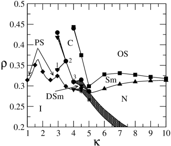
Figure 8: Phase diagram of prolate parallelepipeds. Several phases are labeled like in Figs. 2, 3, and 5 ($N$: nematic and $PS$: plastic solid) and the transition densities are labeled with different symbols (Star: isotropic; diamond: plastic solid; circle: columnar; down triangle: discotic smectic; up triangle: smectic; and square: oriented solid). The shaded areas limit the regions of two phase coexistence. The transitions labeled by by 1,2, and 3 are first order in nature.

The nematic phase begins to be stable for $\kappa>5$ with its stability region bounded below by the first order isotropic-nematic transition and above by a continuous nematic-smectic transition. Finally, the smectic region is bounded above by a continuous transition to the oriented solid phase (see Fig. 8).

Again the nematic-smectic transition points are joined with spinodal lines and for each $\kappa$ a minimization was carried out to check numerically the continuous character of the transition (the smectic solution begins to be stable right at the spinodal). In Ref. Martinez-Raton_5 a bifurcation analysis with the same functional was carried out to study the nature of the nematic-smectic transition. A thermodynamic and mechanical stability analysis showed that the nematic-smectic transition is first order, which is in contradiction with the numerical minimization results presented here. A possible reason that justifies this contradiction could be that the $N$-Sm transition is very weakly first order, so weak that the numerical accuracy used in the functional minimization can not decide about its nature. Another possibility is that the numerical accuracy failure is somewhere in the bifurcation analysis. A careful revision of this analysis is certainly called for in order to settle this point.

The available simulation results for freely rotating hard spherocylinders show that the isotropic phase exhibits a transition to the solid phase for $0\leq\kappa\leq 4.1$ (the solid is plastic for $\kappa\leq 1.35$ and oriented for $1.35\leq\kappa\leq 4.1$) while the isotropic-smectic and nematic-smectic transitions begin at $\kappa=4.1$ and $4.7$, respectively Bolhuis [notice that for hard spherocylinders the length-to-breadth ratio is $\kappa=(L+D)/D$]. We can see that, despite the different particle geometry and the restricted orientations of the Zwanzig model, the agreement for the threshold $\kappa$ at which spatial instabilities to the solid and smectic phase destabilize the homogeneous phases is rather good. Also the qualitative picture is similar: elongated rods form smectics, and more symmetric particles form solids. The main difference between them is that the Zwanzig phase diagram presents regions where the columnar and discotic smectic phases are stable, a difference due to the restriction of orientations.

III.3 Oblate parallelepipeds

The phase diagram of oblate parallelepipeds ($\kappa<1$) is shown in Fig. 9. The main differences after comparing the phase diagrams of prolate (Fig. 8) and oblate particles are that in the latter: (i) The smectic is no more a stable phase. (ii) The region of columnar phase stability is considerably larger. (iii) The stability region of the plastic solid is reduced (in fact this phase is stable only up to $\kappa^{-1}\approx 2.5$) at the expense of that of the discotic smectic phase. (iv) The transitions to the latter are strongly first order in nature (except for $\kappa^{-1}=4.5$). (v) The oriented solid phase is replaced by a perfectly oriented solid in which “$x$” and “$y$” species are absent. This phase, after scaling in the $z$ direction, is the same as the solid of parallel hard cubes. A solution from the FMF minimization with three dimensional spatial modulations and with $\gamma_{\perp}\neq 0$ has not been found in the parallelepipedic unit cell (the case of face-centered or body-centered cubic unit cells have not been tried here).

Finally, similar by to what happens with prolate parallelepipeds, the nematic phase begins to be stable at $\kappa^{-1}\gtrsim 5$. It undergoes a continuous phase transition to the columnar phase (the transition points of Fig. 9 are joined with the spinodal curve).

The parallelepipeds with $\kappa^{-1}=1.5$ exhibit an interesting phase behavior. At low densities the isotropic phase destabilizes with respect to the columnar phase and not with respect to the PS phase. This example shows that the prediction for phase transitions using only the spinodal instability calculations can generate uncertainties about the possible symmetries of the inhomogeneous phases. In fact these calculations do not allow to decide in this example if the new phase is a plastic solid or a columnar phase. Only by a complete minimization of the FMF, could it be concluded that the columnar phase is the stable one.

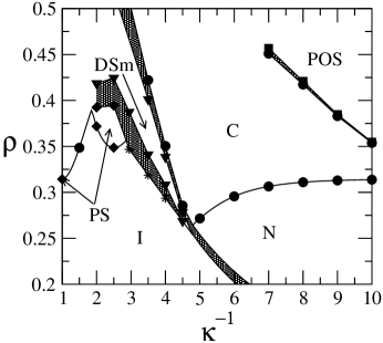
Figure 9: Phase diagram of oblate parallelepipeds (the same symbols and labels of Fig. 8 are used). POS: Perfectly oriented solid.

In Fig. 10 (a) the density profiles of perpendicular [$\rho_{\perp}(z)$] and parallel [$\rho_{\parallel}(z)$] species are shown for the discotic smectic phase of oblate particles with $\kappa^{-1}=2.5$, while the order parameter profile is shown in Fig. 10(b). This discotic smectic phase coexists at $\rho=0.4244$ with the plastic solid phase. The period in units of the large parallelepiped edge length is $d/\sigma=1.2142$. The random orientation of the uniaxial axes within the layers is confirmed by the high negative values of the order parameter at the position of the density peak of the perpendicular species. The main difference between the DSm of Fig. 10 and that of Fig. 7 is that the “z” species is now localized preferentially not at the center of the interlayer space, but near the smectic layers [see Fig. 10(a)], exhibiting two local maxima at each side of the layer. This effect can be explained by the depletion force that the perpendicular species exerts on the parallel one.

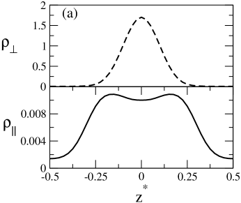
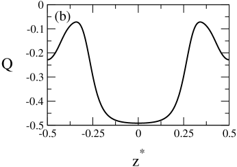
Figure 10: Density (a) and order parameter (b) profiles of the DSm phase coexisting at $\rho=0.4244$ with the PS. (a) Shows the density profiles of perpendicular ($\rho_{\perp}$) and parallel ($\rho_{\parallel}$) species.

The $N$-Sm ($N-C$) and the Sm-OS ($C$-POS) transition lines of Figs. 8 and 9 converge asymptotically to $\rho=0.3143$, the value of the fluid-solid bifurcation density, as $\kappa\to\infty$ ($\kappa^{-1}\to\infty$). The reason for this is that upon increasing $\kappa$ ($\kappa^{-1}$) the number of rods (plates) with orientation perpendicular to the director becomes vanishing small, and then the system is, after rescaling the $z$ direction, almost equivalent to a system of parallel cubes.

Simulations of the Zwanzig model on a $15\times 15\times 15$ lattice with spacing $1/3$ show that oblate parallelepipeds with dimensions $5\times 5\times 1$ undergo a transition to a phase exhibiting a columnar structure Casey at a density somewhere between $0.55<\rho<0.65$. On increasing the system size to $30\times 30\times 30$ the global columnar order disappears, but local correlations persist in the fluid with particle alignment distributed evenly among the three available orientations. In the same work the effect that orientational constraints have on the stability of the inhomogeneous phases was studied. While a system of biaxial $5\times 3\times 1$ “tiles” without orientational constraints (except those inherent to the Zwanzig model) stabilizes in a smectic phase with the shortest edge lengths perpendicular to the layers, the system composed by “tiles” with all their long edge lengths parallel to each other exhibits a phase transition to the smectic phase with these edge lengths perpendicular to the layers, similar to what is found here for uniaxial oblate parallelepipeds (the discotic smectic phase).

Simulations of hard cut spheres show that for $\kappa=0.3$ there is an isotropic-solid transition, for $\kappa=0.2$ an isotropic-columnar transition (the isotropic phase might instead be a peculiar “cubatic” phase) and for $\kappa=0.1$ a nematic-columnar one Veerman . From these results it can be concluded that the effect that the degree of particle anisotropy has on the symmetry of the stable phases for both cut spheres and hard parallelepipeds with restricted orientations, is qualitatively similar.

IV Conclusions

The goal of this article has been the calculation of the phase diagram of the Zwanzig model for prolate and oblate parallelepipeds centering the attention on the phase transitions to inhomogeneous phases. For this purpose the fundamental measure functional for hard parallelepipeds with restricted orientations has been used. This functional is exactly the same for any particle shape (prolate and oblate depending on $\kappa$), which allows for a unified study of the phase behavior of both kinds of particles. A free minimization of the functional was carried out with the only constraints of choosing a parallelepipedic unit cell and of imposing uniaxial symmetry in the inhomogeneous phases. The latter is justified by uniaxial symmetry of the particles. The degree of approximation to the exact density profiles was controlled by the cutoff imposed on the reciprocal lattice numbers in the Fourier expansion of the density profiles.

A system of parallel hard cubes was separately studied, which was motivated by recent simulations on this system Jagla ; Groh . Applying a modified versions of the FMF to improve the description of the PHC liquid, along the same lines as Refs. Tarazona_2 and Roth , the continuous transition point to the solid phase and the equation of state of the solid were calculated from the divergence of the structure factor and from the functional minimization with respect to Gaussian density profiles. Although the transition density and fraction of vacancies change in the right direction, these results are still far from the simulations. In fact, the solid phase is poorly described by the new functional. The poor convergence of the PHC virial series does not make this procedure as effective as for hard spheres. Further refinement of the method and the proper inclusion of vacancies in simulations of the solid phase will probably improve the agreement between theory and simulations.

The original FMF for PHC was minimized to study the relative stability of the smectic, columnar, and solid phases, starting at low densities from the bifurcation point. The solid phase is the only stable phase, followed by the columnar and the smectic (in order of energy stability). At high densities the same behavior is shown from calculations using cell theory, functional minimization with Gaussian density profiles and computer simulations Groh .

The system of prolate and oblate parallelepipeds exhibits a very rich phase behavior. Apart from the plastic or oriented solid, smectic, and columnar phases, which are present also in systems of prolate (spherocylinders Bolhuis ) and oblate (cut spheres Veerman ) particles, a new phase appears: the discotic smectic, the existence of which was confirmed by simulations Casey . The close relation between the particle anisotropy and symmetry of the stable phases (elongated particles form smectics, flattened one form columnars and more isotropic particles form solids) which has been observed in simulations Strobants_1 ; Bolhuis ; Veerman and experiments Maeda is confirmed by this simple model.

There are two important effects that the restriction of orientations has on the phase diagram topology: (i) The already pointed out stability of the discotic smectic. (ii) The stability of the columnar phase of prolate parallelepipeds for some aspect ratios. The structural properties of inhomogeneous phases that were found through functional minimization allow us to elucidate interesting effects such as the microsegregation behavior of different species in the solids and the depletion effect between particles in the smectics. Those findings endorse the predictive power of the FMF in the description of highly inhomogeneous phases.

- (1) L. Onsager, Ann. NY Acad. Sci. 51, 627 (1949).
- (2) R. W. Zwanzig, J. Chem. Phys. 24, 855 (1956); 39, 1714 (1963).
- (3) L. K. Runnels and Carolyn Colvin, J. Chem. Phys. 53, 4219 (1970).
- (4) B. Barboy and W. M. Gelbart, J. Chem. Phys. 71, 3053 (1979).
- (5) B. G. Moore and W. E. MacMullen, J. Phys. Chem. 96, 3374 (1992); J. Chem. Phys. 97, 9267 (1992).
- (6) P. Tarazona, Mol. Phys. 52, 81 (1984).
- (7) G. Rickayzen, Mol. Phys. 75, 333 (1992).
- (8) A. Stroobants, H. N. W. Lekkerkerker, and D. Frenkel, Phys. Rev. A 36, 2929 (1987); D. Frenkel, J. Phys. Chem. 91, 4912 (1987); D. Frenkel, H. N. W. Lekkerkerker, and A. Stroobants, Nature (London) 332, 882 (1988).
- (9) J. A. C. Veerman and D. Frenkel, Phys. Rev. A 45, 5632 (1992).
- (10) P. Bolhuis and D. Frenkel, J. Chem. Phys. 106, 666 (1997).
- (11) A. M. Somoza and P. Tarazona, Phys. Rev. A 41, 965 (1990).
- (12) A. Poniewierski and T. J. Sluckin, Phys. Rev. A 43, 6837 (1991).
- (13) E. Velasco, L. Mederos, and D. E. Sullivan, Phys. Rev. E 62, 3708 (2000).
- (14) H. Graf and H. Lowen, J. Phys.: Condens. Matter 11, 1435 (1999).
- (15) Y. Rosenfeld, Phys. Rev. Lett. 63, 980 (1989).
- (16) Y. Rosenfeld, Phys. Rev. E 50, R3318 (1994).
- (17) A. Chamoux and A. Perera, J. Chem. Phys. 104, 1493 (1996).
- (18) A. Chamoux and A. Perera, J. Chem. Phys. 108, 8172 (1998); S. Dubois and A. Perera, ibid. 116, 6354 (2002).
- (19) G. Cinacchi and F. Schmid, J. Phys.: Condens. Matter 14, 12 223 (2002).
- (20) R. van Roij, M. Dijkstra, and R. Evans, J. Chem. Phys. 113, 7689 (2000); M. Dijkstra, R. Van Roij and R. Evans, Phys. Rev. E 63, 051703 (2001).
- (21) Y. Martínez-Ratón, cond-mat/0212333 (unpublished).
- (22) L. Harnau, D. Rowan, and J.-P. Hansen, J. Chem. Phys. 117, 11 359 (2002); L. Harnau and S. Dietrich, Phys. Rev. E 65, 021505 (2002).
- (23) K. Shundyak and R. van Roij, Phys. Rev. E 69, 021506 (2004).
- (24) J. A. Cuesta and Y. Martínez-Ratón, Phys. Rev. Lett. 78, 3681 (1997); J. Chem. Phys. 107, 6379 (1997).
- (25) P. Tarazona, Phys. Rev. Lett. 84, 694 (2000).
- (26) M. Schmidt, Phys. Rev. E 63, 050201 (2001).
- (27) Y. Martínez-Ratón and J. A. Cuesta, Phys. Rev. Lett. 89, 185701 (2002).
- (28) Y. Martínez-Ratón and J. A. Cuesta, J. Chem. Phys. 118, 10164 (2003).
- (29) M. Bier, L. Harnau, and S. Dietrich, Phys. Rev. E 69, 021506 (2004).
- (30) K. Shundyak and R. van Roij, Phys. Rev. E 68, 061703 (2003).
- (31) A. Casey and P. Harrowell, J. Chem. Phys. 103, 6143 (1995).
- (32) Y. Martínez-Ratón and J. A. Cuesta, J. Chem. Phys. 111, 317 (1999).
- (33) E. A. Jagla, Phys. Rev. E 58, 4701 (1998).
- (34) B. Groh and B. Mulder, J. Chem. Phys. 114, 3653 (2001).
- (35) F. van Swol and L. V. Woodcock, Mol. Simul. 1, 95 (1987).
- (36) P. Tarazona, Physica A 306, 243 (2002).
- (37) R. Roth, R. Evans, A. Lang, and G. Kahl, J. Phys.: Condens. Matter 14, 12063 (2002).
- (38) L. Lafuente and J. A. Cuesta, Phys. Rev. Lett. 89, 145701 (2002).
- (39) A. Stroobants, Phys. Rev. Lett. 69, 2388 (1992).
- (40) J. M. Polson and D. Frenkel, Phys. Rev. E 56, R6260 (1997).
- (41) F. M. van der Kooij and H. N. W. Lekkerkerker, Phys. Rev. Lett. 84, 781 (2000).
- (42) Y. Martínez-Ratón, J. A. Cuesta, R. Van Roij and B. Mulder, in New Approaches to Problems in Liquid State Theory (Kluwer Academic, Dordrecht, 1999), Vol. 529, p. 139.
- (43) H. Maeda and Y. Maeda, Phys. Rev. Lett 90, 018303 (2003).