Geometrical vs. Fortuin-Kasteleyn Clusters
in the
Two-Dimensional $q$-State Potts Model

Abstract

The tricritical behavior of the two-dimensional $q$-state Potts model with vacancies for $0\leq q\leq 4$ is argued to be encoded in the fractal structure of the geometrical spin clusters of the pure model. The known close connection between the critical properties of the pure model and the tricritical properties of the diluted model is shown to be reflected in an intimate relation between Fortuin-Kasteleyn and geometrical clusters: The same transformation mapping the two critical regimes onto each other also maps the two cluster types onto each other. The map conserves the central charge, so that both cluster types are in the same universality class. The geometrical picture is supported by a Monte Carlo simulation of the high-temperature representation of the Ising model ($q=2$) in which closed graph configurations are generated by means of a Metropolis update algorithm involving single plaquettes.

1 Introduction

The two-dimensional $q$-state Potts models [1] can be equivalently formulated in terms of Fortuin-Kasteleyn (FK) clusters of like spins [2]. These FK clusters are obtained from the geometrical spin clusters, which consist of nearest neighbor sites with their spin variables in the same state, by laying bonds with a certain probability between the nearest neighbors. The resulting FK, or bond clusters are in general smaller than the geometrical ones and also more loosely connected. The FK formulation of the Potts models can be thought of as a generalization of (uncorrelated) bond percolation, which obtains in the limit $q\to 1$. The geometrical clusters themselves arise in the low-temperature representation of the pure model [3].

For $q\leq 4$, where the model undergoes a continuous phase transition, the FK clusters percolate at the critical temperature and their fractal structure encodes the complete critical behavior. The thermal critical exponents are obtained using the cluster definitions from percolation theory [4]. With clusters and their fractal properties taking the central stage, the FK formulation provides a geometrical description of the Potts model.

The concept of correlated bond percolation has been turned into a powerful Monte Carlo algorithm by Swendsen and Wang [5], and by Wolff [6], in which not individual spins are updated, but entire FK clusters. The main advantage of the nonlocal cluster update over a local spin update, like Metropolis or heat bath, is that it drastically reduces the critical slowing down near the critical point.

Although it was known from the relation with other statistical models that the phase transition of the Potts models changes from being continuous to first order at $q=4$ [7], initial renormalization group approaches failed to uncover the first-order nature for larger $q$. Only after the pure model was extended to include vacant sites, this feature was observed [8]. In a Kadanoff block-spin transformation, the vacant sites represent blocks without a majority of spins in a certain state, i.e., they represent disordered blocks. In addition to the pure Potts critical behavior, the site diluted model also displays tricritical behavior, which was found to be intimately connected with the critical behavior [8]. With increasing $q$, the critical and tricritical fixed points move together until at $q=4$ they coalesce and the continuous phase transition turns into a first-order one.

Recently, the cluster boundaries of two-dimensional critical systems have been intensively studied by means of a method dubbed “stochastic Loewner evolution” (SLE${}_{\bar{\kappa}}$)–a one-parameter family of random conformal maps, introduced by Schramm [9]. In this approach, the Brownian motion of a random walker is described by Loewner’s ordinary differential equation, containing a random term whose strength is specified by a parameter $\bar{\kappa}\geq 0$ [10]. Different values of $\bar{\kappa}$ define different universality classes. Various results previously conjectured on the basis of the Coulomb gas map [11, 12, 13] and conformal invariance [14] have been rigorously established by this method. The interrelation between SLE${}_{\bar{\kappa}}$ traces and the Coulomb gas description is made explicit by observing that the Coulomb gas coupling parameter $g$ can be simply expressed by $g=1/\bar{\kappa}$ [15]. The nature of the SLE${}_{\bar{\kappa}}$ traces changes with $\bar{\kappa}$: for $0\leq\bar{\kappa}<1$ the path is simple (non-intersecting), while for $1\leq\bar{\kappa}\leq 2$ it possesses double points (see Fig. 1); and for $\bar{\kappa}>2$ it is space-filling [16, 17].

Figure 1: Trace possessing a double point.

This change reflects a change in the critical systems described by the SLE${}_{\bar{\kappa}}$ traces [15]: For $1\leq\bar{\kappa}\leq 2$ they represent the hulls of FK clusters of the $q$-state Potts model with $4\geq q\geq 0$, while for $\frac{1}{2}\leq\bar{\kappa}\leq 1$ they represent the closed graphs of the high-temperature representation of the O($n$) model with $-2\leq n\leq 2$ and at the same time also the external perimeters of FK clusters with dual parameter $1/\bar{\kappa}$ [15, 18]. For a recent overview from the mathematical point of view, see Ref. [18].

In this paper, the tricritical regime of the two-dimensional (annealed) site diluted $q$-state Potts model with $0\leq q\leq 4$ is studied from the geometrical point of view. It will be argued that the tricritical behavior of these models is encoded in the geometrical clusters of the pure Potts model in the same way that the critical behavior is encoded in the FK clusters. The relation between geometrical clusters and tricritical behavior was first established by Stella and Vanderzande [19, 20] for the special case $q=2$, i.e., for the Ising model. Using arguments based on renormalization group, conformal invariance, and numerical simulations, they showed that the geometrical cluster dimensions of the Ising model at criticality are determined by the $q=1$ tricritical Potts model, as was earlier conjectured by Temesvári and Herényi [21]. The values of two of the three leading tricritical exponents characterizing the geometrical clusters were already determined before by Coniglio and Klein [22]. The distinctive feature of the $q=1$ tricritical model is that it is in the same universality class as the Ising model defined by the central charge $c=\frac{1}{2}$. In addition, it has the same correlation length exponent $\nu=1$ as the Ising model. The boundaries of geometrical Potts clusters were also already known to be in the same universality class as the tricritical model with the same central charge [23, 13]. Formulated in terms of SLE${}_{\bar{\kappa}}$ traces, the hulls of geometrical clusters are described at criticality by traces with $\frac{1}{2}\leq\bar{\kappa}\leq 1$, thereby forming the geometrical counterpart of the FK hulls which are described by the traces with $1\leq\bar{\kappa}\leq 2$. It will be shown here that not just the boundary dimensions, but all the relevant fractal dimensions characterizing FK clusters are in one-to-one correspondence with those of the geometrical clusters, thus providing a physical picture for the close connection between the critical and tricritical behaviors just mentioned. The important aspect of the map is that it leaves the central charge unchanged, so that both cluster types and their boundaries are in the same universality class, characterized by the same central charge.

To support this geometrical picture, we carry out a Monte Carlo study of the high-temperature representation of the 2-state Potts, or Ising model. We generate the high-temperature graphs by using a Metropolis update algorithm involving single plaquettes [24]. By duality, the high-temperature graphs, which are closed, form the hulls of geometrical spin clusters on the dual lattice. We thus simulate the geometrical hulls directly without first considering the clusters. From the geometrical properties of these graphs, such as their distribution, the size of the largest graph, and whether or not a graph spans the lattice, the fractal dimension of the hulls of geometrical clusters can be determined immediately. Our numerical result agrees with the analytic prediction by Duplantier and Saleur [25], which was derived using the Coulomb gas map.

The paper is organized as follows. In Sec. 2, those aspects of the diluted $q$-state Potts model are reviewed that are of relevance for the following, in particular its cluster properties. Section 3.1 discusses the various fractal dimensions characterizing FK clusters. In Sec. 3.2, the results for FK clusters are transcribed to geometrical clusters, which in Sec. 4 are shown to encode the tricritical Potts behavior. The Monte Carlo results for the high-temperature representation of the Ising model are presented in Sec. 5, followed by a summary in Sec. 6.

2 Diluted $q$-state Potts Model

The diluted Potts model can be defined by the Hamiltonian [26]:

$$-\beta\mathcal{H}=K\sum_{\langle ij\rangle}(\delta_{\sigma_{i},\sigma_{j}}-1)+J\sum_{\langle ij\rangle}(\delta_{\tau_{i},\tau_{j}}-1)\delta_{\sigma_{i},\sigma_{j}}-H\sum_{i}(\delta_{\tau_{i},1}-1),$$ (1)

where $\beta$ denotes the inverse temperature and the double sum $\sum_{\langle ij\rangle}$ extends over nearest neighbors only. The first term at the right hand with coupling constant $K$ is the pure $q$-state Potts model with spin variable $\sigma_{i}=1,2,\cdots,q$ at the $i$th site. On this a second Potts model with auxiliary spin variable $\tau_{i}=1,2,\cdots,s$, coupling constant $J$, and ghost field $H$ is superimposed. The reasons for this extension of the pure Potts model are twofold. First, in the limit $s\to 1$, the $s$-state Potts model describes (bond) percolation [2], which is naturally formulated in terms of clusters. The extension thus allows for the investigation of cluster properties of the original model when the limit $s\to 1$ is taken. Second, the diluted model has two fixed points for $q\leq 4$. In addition to the pure Potts critical point, it also has a tricritical point, depending on the value of the coupling constant $J$. Adding vacancies therefore leads to two distinct scaling regimes, each with its own critical exponents. Note that the limit $s\to 1$ is subtle as precisely for $s=1$, the Hamiltonian (1) is independent of $J$ and $H$, so that it reduces to the standard Potts model.

The second term in the Hamiltonian (1) connects nearest neighbors of like spins (for which $\delta_{\sigma_{i},\sigma_{j}}=1$) with bond probability

$$p=1-{\rm e}^{-J},$$ (2)

while the ghost field $H$ in the last term acts as a chemical potential for the auxiliary spins in the first state, $\tau_{i}=1$. A configuration of auxiliary bonds thus obtained can be represented by a graph on a restricted lattice, consisting of those sites of the original lattice that have at least one nearest neighbor with like spins (see Fig. 2).

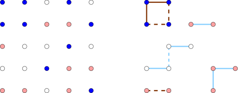
Figure 2: Left panel: Original lattice with the spin variables taking three different values ($q=3$) indicated by different grey scales. Right panel: Reduced lattice consisting of sites having at least one nearest neighbor with like spin, i.e., of the same shading. Auxiliary bonds, taking two different values ($s=2$), are laid with a certain probability within clusters of like spins. The resulting bond clusters represent sites which are all in the same spin (indicated by dots with the same shading) and auxiliary spin state (indicated by bonds with the same shading). The broken bonds within a spin cluster are indicated by broken lines.

Following Fortuin and Kasteleyn [2], we can rewrite the partition function of the model (1) as [26]

$$Z=\sum_{\{\sigma\}}\exp\left[K\sum_{\langle ij\rangle}(\delta_{\sigma_{i},\sigma_{j}}-1)\right]\sum_{\{\Gamma\}}p^{b}(1-p)^{\bar{b}}\prod_{\mathcal{C}(\Gamma)}\left[1+(s-1){\rm e}^{-Hn_{c}}\right],$$ (3)

where $\{\Gamma\}$ denotes the set of bond configurations specified by $b$ bonds and $\bar{b}$ broken bonds between like spins, while $\mathcal{C}(\Gamma)$ denotes the clusters in a given bond configuration $\Gamma$. Finally, $n_{c}$ is the number of sites contained in the $c$th cluster, where an isolated single site counts as a cluster, irrespective of whether it is on the restricted or the original lattice. This last observation follows from the absence of any reference to the spin variable in the last term of the Hamiltonian (1). In the partition function, the limiting case $s=1$, where the Hamiltonian (1) is independent of $J$ and $H$, can be recovered by noting that, for a given spin configuration the sum $\sum_{\{\Gamma\}}p^{b}(1-p)^{\bar{b}}$ of the probabilities of all possible bond configurations adds up to unity.

As mentioned above, cluster properties can be extracted from the partition function (3) of the diluted model by taking the limit $s\to 1$. Specifically [26],

$$\left.\frac{1}{N}\frac{{\rm d}\ln Z}{{\rm d}s}\right|_{s=1}=\frac{1}{N}\left\langle\sum_{\{\Gamma\}}p^{b}(1-p)^{\bar{b}}\prod_{\mathcal{C}(\Gamma)}{\rm e}^{-Hn_{c}}\right\rangle=\sum_{n}\ell_{n}{\rm e}^{-Hn},$$ (4)

where $N$ denotes the total number of lattice sites and $\ell_{n}$ is the cluster distribution giving the average number density of clusters of $n$ sites. The thermal average indicated by angle brackets in Eq. (4) is taken with respect to the pure $q$-state Potts model, i.e., the first factor in the Hamiltonian (1). The right hand is seen to be the generating function for clusters. By differentiating it with respect to the ghost field $H$ higher momenta in the cluster sizes can be obtained.

The pure Potts part of the theory is easily dealt with by noting that, for a given spin configuration, it gives a factor $\left({\rm e}^{-K}\right)^{a}$, where $a$ denotes the number of nearest neighbor pairs of unlike spin.

The two fixed points of the diluted model correspond to two specific choices of the coupling constant $J$ [22, 27] with $K$ fixed at the critical temperature $K_{\mathrm{c}}$ of the pure Potts model (see Fig. 3).

\psfrag{K}[t][t][.8][0]{$K$}\psfrag{kc}[t][t][.8][0]{$K_{c}$}\psfrag{p}[t][t][.8][0]{$p$}\psfrag{Geo}[l][t][.8][0]{Geometrical}\psfrag{FK}[l][t][.8][0]{FK}\includegraphics[width=85.35826pt]{phasediagram}

Figure 3: Phase diagram of the diluted model (1) in the $K$-$p$ plane, with $p=1-\exp(-J)$ the bond probability. The arrows indicate the renormalization flow in the infrared. The FK fixed point governs the critical behavior described by the FK clusters, while the geometrical fixed point governs the tricritical behavior described by the geometrical clusters.

The first choice is obtained by taking $J=K$. This case is special because the factors ${\rm e}^{-K}$ arising from the first term in the Hamiltonian (1) can now be related to the bond probability (2) as

$${\rm e}^{-K}=1-p,$$ (5)

and the partition function becomes

$$Z_{\rm FK}=\sum_{\{\Gamma\}}p^{b}(1-p)^{B-b}\prod_{\mathcal{C}(\Gamma)}\left[1+(s-1){\rm e}^{-Hn_{c}}\right]q,$$ (6)

where $B$ is the total number of bonds on the lattice, $B=b+\bar{b}+a$. The sum $\sum_{\{\sigma\}}$ produced the factor $q$ since each cluster can be in any of the $q$ spin states. For $s=1$, this partition function reduces to the celebrated Fortuin-Kasteleyn representation of the Potts model [2],

$$Z_{\rm FK}=\sum_{\{\Gamma\}}p^{b}(1-p)^{B-b}q^{N_{\mathrm{C}}},$$ (7)

where $N_{\mathrm{C}}$ is the number of clusters, including isolated sites, contained in the bond configuration $\Gamma$. The clusters seen in the limit $s\to 1$ encode the complete thermal critical behavior of the model and are frequently referred to as Fortuin-Kasteleyn (FK) clusters. For $q\to 1$, the partition function (7) describes standard, uncorrelated percolation, where the FK clusters coincide with the usual percolation clusters.

The second choice is obtained by taking the limit $J\to\infty$ where the bond probability $p$ tends to unity. The only clusters surviving this limit are those without any broken bonds between like spins ($\bar{b}=0$), which are the geometrical clusters. The partition function can be written in this limit as

$$Z_{\rm G}=\sum_{\{\Gamma\}}{\rm e}^{-Ka}\prod_{\mathcal{C}(\Gamma)}\left[1+(s-1){\rm e}^{-Hn_{c}}\right]P_{c}(q),$$ (8)

where the factor $P_{c}(q)$ is such that the product over the clusters $\prod_{\mathcal{C}(\Gamma)}P_{c}(q)=:P_{\Gamma}(q)$ gives the number of different spin configurations for a given bond configuration $\Gamma$. That is, $P_{\Gamma}(q)$ is the number of $q$-colorings of the geometrical clusters contained in $\Gamma$, where it is recalled that an isolated single site counts as a cluster. For $s=1$, the partition function reduces to

$$Z_{\rm G}=\sum_{\{\Gamma\}}{\rm e}^{-Ka}P_{\Gamma}(q),$$ (9)

which is nothing but the standard low-temperature representation of the pure Potts model [3]. For the Ising model ($q=2$), each graph can be colored in two different ways, $P_{\Gamma}(2)=2$, so that the coloring number becomes irrelevant. For uncorrelated percolation ($q=1$), $P_{\Gamma}(1)=1$ and $a=0$ trivially, so that only one geometrical cluster remains, representing a fully occupied lattice [27].

3 Pure Potts Model

3.1 FK Clusters

Adapting similar notations [12], we parameterize the two-dimensional $q$-state Potts models as

$$\sqrt{q}=-2\cos(\pi/\bar{\kappa}),$$ (10)

with $2\geq\bar{\kappa}\geq 1$ so that the argument of the cosine takes values in the interval $[\pi/2,\pi]$. Special cases are:

• tree percolation ($q=0,\;\bar{\kappa}=2$)

• uncorrelated percolation ($q=1,\;\bar{\kappa}=\frac{3}{2}$)

• Ising model ($q=2,\;\bar{\kappa}=\frac{4}{3}$)

• $q=3,\;\bar{\kappa}=\frac{6}{5}$

• $q=4,\;\bar{\kappa}=1$.

The parameter $\bar{\kappa}$ is related to the central charge $c$ via [14]

$$c=1-\frac{6(1-\bar{\kappa})^{2}}{\bar{\kappa}},$$ (11)

while the correlation length exponent $\nu$ and the Fisher exponent $\eta_{\mathrm{C}}$ are given by [11]:

$$\nu=\frac{2}{3}\frac{1}{2-\bar{\kappa}},\quad\eta_{\mathrm{C}}=2-\frac{1}{\bar{\kappa}}-\frac{3}{4}\bar{\kappa}.$$ (12)

The latter determines the algebraic decay of the cluster correlation function $G_{\mathrm{C}}({\bf x})$ at the critical point:

$$G_{\mathrm{C}}({\bf x},{\bf x}^{\prime})\sim 1/|{\bf x}-{\bf x}^{\prime}|^{d-2+\eta_{\mathrm{C}}},$$ (13)

with $d$ the number of space dimensions. Physically, $G_{\mathrm{C}}({\bf x},{\bf x}^{\prime})$ gives the probability that sites ${\bf x}$ and ${\bf x}^{\prime}$ belong to the same cluster. The subscript “C” is to distinguish the thus defined exponent from the standard definition based on the spin-spin correlation function. The other exponents can be obtained from the two given in Eq. (12) using standard scaling relations.

For ease of comparison with the more often used notation where the central charge is given in terms of a parameter $m$ [14]:

$$c=1-\frac{6}{m(m+1)},$$ (14)

which in turn is related to $q$ through

$$\sqrt{q}=2\cos\left(\frac{\pi}{1+m}\right)=-2\cos\left(\frac{m}{1+m}\pi\right),$$ (15)

with $1\leq m\leq\infty$, we note that the relation with $\bar{\kappa}$ reads for Potts models:

$$\bar{\kappa}=\frac{1+m}{m},\quad m=\frac{1}{\bar{\kappa}-1}.$$ (16)

Usually, only the first equation in Eq. (15) is given, we included the second to clearly see the relation with the $\bar{\kappa}$ parameterization.

The critical behavior of the Potts model is also encoded in the FK cluster distribution $\ell_{n}$ given in Eq. (4), which near the critical point takes the form

$$\ell_{n}\sim n^{-\tau_{\rm C}}\exp(-\theta n),$$ (17)

as in percolation theory [4]. The first factor, characterized by the exponent $\tau_{\rm C}$, is an entropy factor, measuring the number of ways of implementing a cluster of given size on the lattice. The second factor is a Boltzmann weight which suppresses large clusters as long as the parameter $\theta$ is finite. When the critical temperature is approached from above, it vanishes as $\theta\propto(T-T_{\rm c})^{1/\sigma_{\rm C}}$, with $\sigma_{\rm C}$ a second exponent. The cluster distribution then becomes algebraic, meaning that clusters of all sizes are present. As in percolation theory [4], the values of the two exponents specifying the cluster distribution uniquely determine the critical exponents as

$$\alpha =2-\frac{\tau_{\rm C}-1}{\sigma_{\rm C}}, \beta_{\rm C} =\frac{\tau_{\rm C}-2}{\sigma_{\rm C}}, \gamma_{\rm C} =\frac{3-\tau_{\rm C}}{\sigma_{\rm C}},$$

$$\eta_{\rm C} =2+d\frac{\tau_{\rm C}-3}{\tau_{\rm C}-1}, \nu =\frac{\tau_{\rm C}-1}{d\sigma_{\rm C}}, D_{\mathrm{C}} =\frac{d}{\tau_{\rm C}-1},$$ (18)

where the fractal dimension of the clusters is related to the Fisher exponent (12) via

$$D_{\mathrm{C}}=\tfrac{1}{2}(d+2-\eta_{\rm C}).$$ (19)

Various exponents are given the subscript “C” to indicate that the cluster definition is used in defining them. For FK clusters, where in terms of $\bar{\kappa}$

$$\sigma_{\rm C}=\frac{12\bar{\kappa}(2-\bar{\kappa})}{3\bar{\kappa}^{2}+8\bar{\kappa}+4},\quad\tau_{\rm C}=\frac{3\bar{\kappa}^{2}+24\bar{\kappa}+4}{3\bar{\kappa}^{2}+8\bar{\kappa}+4},$$ (20)

the cluster exponents coincide with the thermal ones. The cluster definition not always yields the thermal critical exponents. For example, when the critical behavior of a system allows for a description in terms of other geometrical objects such as closed particle worldlines or vortex loops, a related but different definition is required to obtain the thermal exponents from the loop distribution [28].

The various fractal dimensions characterizing FK clusters and the leading thermal eigenvalue $y_{T}=1/\nu$ read in terms of $\bar{\kappa}$ [13, 29, 30]

$$D_{\mathrm{C}} = 1+\frac{1}{2\bar{\kappa}}+\frac{3}{8}\bar{\kappa}$$ (21a)

$$D_{\mathrm{H}} = 1+\frac{\bar{\kappa}}{2}$$ (21b)

$$D_{\mathrm{EP}} = 1+\frac{1}{2\bar{\kappa}}$$ (21c)

$$D_{\mathrm{RB}} = 1-\frac{3}{2\bar{\kappa}}+\frac{\bar{\kappa}}{2}$$ (21d)

$$y_{T} = 3-\frac{3}{2}\bar{\kappa}.$$ (21e)

Here, $D_{\mathrm{C}}$ is the fractal dimension of the clusters themselves, and $D_{\rm H}$ that of their hulls [31, 32]. In the context of uncorrelated percolation, the hull of a cluster can be defined as a biased random walk [31]: Identify two endpoints on a given cluster. Starting at the lower endpoint, the walker first attempts to move to the nearest neighbor to its left. If that site is vacant the walker attempts to move straight ahead. If that site is also vacant, the walker attempts to move to its right. Finally, if also that site is vacant, the walker returns to the previous site, discards the direction it already explored and investigates the (at most two) remaining directions in the same order. When turning left or right, the walker changes its orientation accordingly. The procedure is repeated iteratively until the upper endpoint is reached. To obtain the other half of the hull, the entire algorithm is repeated for a random walker that attempts to first move to its right instead of to its left. The hull of FK clusters is a self-intersecting path. As remarked in the Introduction, these hulls for $4\geq q\geq 0$ correspond to the SLE${}_{\bar{\kappa}}$ traces with $1\leq\bar{\kappa}\leq 2$.

The fractal dimension $D_{\rm EP}$ characterizes the external perimeter. Its operational definition [31] in the context of uncorrelated percolation is similar to that for the hull with the proviso that the random walker only visits (nearest neighbor) vacant sites around the hull of the cluster. From the resulting trace those sites not belonging to the perimeter, i.e., without an occupied site as nearest neighbor, are deleted (such sites can, for example, be visited by the walker when it makes a right or left turn on a square lattice). This leads to non-intersecting traces.

These algorithms have recently been used in a numerical study carried out on fairly large lattices ($L=2^{12}=4096$) to determine the fractal dimensions of FK clusters of the $q$-state Potts models with $q=1,2,3,4$ [33].

By construction, the external perimeter is smoother than the hull, or at least as smooth, so that $D_{\rm EP}\leq D_{H}$. The two are equal when the fractal dimension $D_{\rm RB}$ of the so-called red bonds [34] is negative. (A red bond denotes a bond that upon cutting leads to a splitting of the cluster.) For FK clusters, $D_{\rm EP}$ is strictly smaller than $D_{\rm H}$ for all $1<\bar{\kappa}\leq 2$, while for $\bar{\kappa}=1$ ($q=4$), the fractal dimension of the red bonds becomes zero, and the hull and the external perimeter have identical dimensions.

The two boundary dimensions are seen to satisfy the relation [30]

$$(D_{\mathrm{EP}}-1)(D_{\mathrm{H}}-1)=\tfrac{1}{4}.$$ (22)

An analogous relation, this time also involving the fractal dimension of the FK clusters themselves reads

$$(D_{\mathrm{C}}-D_{\mathrm{EP}})(D_{\mathrm{C}}-\tfrac{3}{4}D_{\mathrm{H}}-\tfrac{1}{4})=\tfrac{3}{16}.$$ (23)

In addition, the fractal dimensions satisfy the linear relation

$$D_{\mathrm{C}}-D_{\mathrm{H}}=\tfrac{1}{4}(D_{\mathrm{EP}}-D_{\mathrm{RB}}).$$ (24)

The dimension $D_{\mathrm{C}}$ of the FK clusters approaches the number of available dimensions, $D_{\rm C}\to 2$ when $q\to 0$ ($\bar{\kappa}\to 2$). In this limit, also the hulls of the FK clusters become space-filling, $D_{\rm H}\to 2$.

As in percolation theory [34], the fractal dimensions can be identified with renormalization group eigenvalues of certain operators. For example, the fractal dimension $D_{\mathrm{C}}$ of the FK clusters coincides with the magnetic scaling exponent $y_{H}$,

$$D_{\mathrm{C}}=y_{H}=d-\beta_{\mathrm{C}}/\nu,$$ (25)

while that of the red bonds, $D_{\rm RB}$, coincides with the eigenvalue $y_{J}$ in the $J$ direction,

$$D_{\rm RB}=y_{J},$$ (26)

and therefore describes the crossover between FK and geometrical clusters [19, 29]. Specifically, $1/y_{J}$ determines the divergence of the correlation length $\xi$ at the critical temperature $K_{\mathrm{c}}$ when the bond probability (2) approaches the critical value $p_{\mathrm{c}}=1-\exp(-J_{\mathrm{c}})$, i.e., $\xi\sim(p_{\mathrm{c}}-p)^{-1/y_{J}}$.

3.2 Geometrical Clusters

Starting from the FK cluster dimensions (21), we next wish to obtain the analog expressions for the geometrical clusters of the Potts model at criticality. As argued by Vanderzande [27], both cluster types are characterized by the same central charge $c$. From Eq. (11) it follows that a given value of $c$ does not uniquely determine $\bar{\kappa}$. Indeed, inverting that equation, we obtain two solutions for $\bar{\kappa}$:

$$\bar{\kappa}_{\pm}=\frac{13-c\pm\sqrt{(c-25)(c-1)}}{12},$$ (27)

with $\bar{\kappa}_{+}\geq 1$ and $\bar{\kappa}_{-}\leq 1$. The solutions satisfy the constraint

$$\bar{\kappa}_{+}\bar{\kappa}_{-}=1.$$ (28)

Since the right hand is independent of $c$, replacing $\bar{\kappa}$ with $1/\bar{\kappa}$ leaves the central charge unchanged, $c({\bar{\kappa}})=c(1/{\bar{\kappa}})$.

As an aside, note that the fractal dimensions of the hull and external perimeter of FK clusters are related by precisely this map [30], which is called duality in SLE studies. This duality, which in the Coulomb gas language corresponds to the earlier observed correspondance $g\to 1/g$ (recall that $g=1/\bar{\kappa}$) [15, 18], is also at the root of the relation (22) between the two boundary dimensions.

Applying the duality map $\bar{\kappa}\to 1/\bar{\kappa}$ to the FK cluster dimensions listed in Eq. (21), we obtain

$$D_{\mathrm{C}}^{\rm G} = 1+\frac{3}{8\bar{\kappa}}+\frac{\bar{\kappa}}{2}$$ (29a)

$$D^{\rm G}_{\mathrm{H}} = 1+\frac{1}{2\bar{\kappa}}$$ (29b)

$$D^{\rm G}_{\mathrm{RB}} = 1+\frac{1}{2\bar{\kappa}}-\frac{3}{2}\bar{\kappa}$$ (29c)

$$y^{\rm G}_{T} = 3-\frac{3}{2\bar{\kappa}},$$ (29d)

where $\bar{\kappa}=\bar{\kappa}_{+}$. These dimensions precisely match those conjectured by Vanderzande for geometrical clusters [27]. We therefore conclude that the geometrical clusters of the Potts model are images of the FK clusters under the map $\bar{\kappa}\to 1/\bar{\kappa}$ for given $\bar{\kappa}$. Since this transformation at the same time maps the critical onto the tricritical regime (see below), it follows that the geometrical clusters (of the pure Potts model) describe the tricritical behavior in the same way as the FK clusters describe the critical behavior. For $\bar{\kappa}=1$ ($q=4$), the dimensions of the FK and geometrical clusters become degenerate, and the critical and tricritical behaviors merge. For $q>4$, the phase transition is discontinuous [7]. The fractal dimension (29a) was first given by Stella and Vanderzande [19] for the Ising case, and generalized to arbitrary $1\leq\bar{\kappa}\leq 2$ by Duplantier and Saleur [35].

The external perimeter dimension $D_{\rm EP}$ of FK clusters has no image under the map $\bar{\kappa}\to 1/\bar{\kappa}$. To understand this, recall that by smoothing the hull of a FK cluster one obtains its external perimeter. For geometrical clusters, on the other hand, the fractal dimension of the red bonds is negative $D_{\rm RB}\leq 0$ as follows from Eq. (29c) with $1\leq\bar{\kappa}\leq 2$, so that $D^{\rm G}_{\rm H}=D^{\rm G}_{\rm EP}$ and the hull of a geometrical cluster is already non-intersecting. This is also reflected by the SLE${}_{\bar{\kappa}}$ traces. Under the transformation $\bar{\kappa}\to 1/\bar{\kappa}$, the self-intersecting traces with $\bar{\kappa}\geq 1$, representing the hulls of FK clusters are mapped onto simple traces with $\bar{\kappa}\leq 1$, representing the hulls of geometrical clusters [15].

For given $\bar{\kappa}$, the fractal dimension of the external perimeters of FK clusters coincides with that of the hulls of geometrical clusters, $D_{\rm EP}=D^{\rm G}_{\rm H}(=D^{\rm G}_{\rm EP})$. Since FK clusters are obtained from geometrical clusters by breaking bonds between nearest neighbors with like spins, the smoothing of the FK hulls apparently undoes this process again (as far as the boundaries are concerned).

Table 1 summarizes the various fractal dimensions appearing in the Potts models. Note that for $q=0$, the geometrical cluster dimension is larger than the number of available dimensions, $D_{\rm C}^{\rm G}>2$, making the geometrical clusters unphysical in this case. The equality $D_{\rm EP}=D_{\rm RB}$ is typical for tree percolation. The value $D^{\rm G}_{\rm C}=2$ for $q=1$ agrees with the observation that in this case the geometrical cluster represents a fully occupied lattice [27]. The cluster dimension $D_{\rm C}(\bar{\kappa})$ possesses a minimum at $1<\bar{\kappa}=2/\sqrt{3}<\frac{4}{3}$, allowing the models with $q=4$ and $q=2$ to have the same dimension.

Table 1: FK and geometrical fractal dimensions characterizing the $q$-state Potts models, with $q=0,1,2,3,4$.

$q$	$c$	$m$	$\bar{\kappa}$	$D_{\rm C}$	$D_{\rm H}$	$D_{\rm EP}$	$y_{T}$	$D_{\rm RB}$	$D_{\rm C}^{\rm G}$	$D_{\rm H}^{\rm G}$	$y^{\rm G}_{T}$	$D_{\rm RB}^{\rm G}$
0	$-2$	1	$2$	$2$	$2$	$\frac{5}{4}$	$0$	$\frac{5}{4}$	$\frac{35}{16}$	$\frac{5}{4}$	$\frac{9}{4}$	$-\frac{7}{4}$
1	$0$	2	$\frac{3}{2}$	$\frac{91}{48}$	$\frac{7}{4}$	$\frac{4}{3}$	$\frac{3}{4}$	$\frac{3}{4}$	$2$	$\frac{4}{3}$	$2$	$-\frac{11}{12}$
2	$\frac{1}{2}$	3	$\frac{4}{3}$	$\frac{15}{8}$	$\frac{5}{3}$	$\frac{11}{8}$	$1$	$\frac{13}{24}$	$\frac{187}{96}$	$\frac{11}{8}$	$\frac{15}{8}$	$-\frac{5}{8}$
3	$\frac{4}{5}$	5	$\frac{6}{5}$	$\frac{28}{15}$	$\frac{8}{5}$	$\frac{17}{12}$	$\frac{6}{5}$	$\frac{7}{20}$	$\frac{153}{80}$	$\frac{17}{12}$	$\frac{7}{4}$	$-\frac{23}{60}$
4	$1$	$\infty$	1	$\frac{15}{8}$	$\frac{3}{2}$	$\frac{3}{2}$	$\frac{3}{2}$	$0$	$\frac{15}{8}$	$\frac{3}{2}$	$\frac{3}{2}$	$0$

The physical meaning of the thermal eigenvalue $y^{\rm G}_{T}$ is related to the existence of a critical magnetic field $H_{\mathrm{s}}(K)$, such that in the region $K<K_{\mathrm{c}}$, $H>H_{\mathrm{s}}(K)$ a geometrical cluster spanning the lattice (hence the subscript “s”) is always present. The eigenvalue $y^{\rm G}_{T}$ namely determines the vanishing of this field as $K$ approaches $K_{\mathrm{c}}$ from below [19]:

$$H_{\mathrm{s}}(K)\sim(K_{\mathrm{c}}-K)^{y^{\rm G}_{T}}.$$ (30)

4 Tricritical Potts Model

In the traditional representation in terms of the parameter $m$ determining the central charge $c$ through Eq. (14), the $q$-state tricritical Potts models is parameterized by [14]

$$\sqrt{q}=2\cos\left(\frac{\pi}{m}\right)=-2\cos\left(\frac{1+m}{m}\pi\right),$$ (31)

where $m$ is restricted to $1\leq m\leq\infty$. As for the Potts models, usually only the first equation is given. The second one is included because on comparing with the parameterization (15) of the Potts models, we observe that the two are related by inverting $m/(1+m)$. Given the connection (16) with the $\bar{\kappa}$ notation, it follows that this is nothing but the central-charge conserving map $\bar{\kappa}\to 1/\bar{\kappa}$ which relates the FK and geometrical clusters of a given Potts model. Whereas $\bar{\kappa}_{+}$ parameterizes the Potts branch (10), the solution $\bar{\kappa}_{-}$ of Eq. (27) parameterizes the tricritical branch,

$$\sqrt{q}=-2\cos(\pi/\bar{\kappa}_{-}),$$ (32)

with $\bar{\kappa}_{-}$ restricted to the values $\frac{1}{2}\leq\bar{\kappa}_{-}\leq 1$, so that the argument of the cosine now takes values in the interval $[\pi,3\pi]$. (From now on, the $\bar{\kappa}$’s are given a subscript plus or minus to indicate the solution larger or smaller than 1. Up to this point only the larger solution was used and no index was needed to distinguish.) The results obtained for the Potts models can be simply transcribed to the tricritical models, provided $\bar{\kappa}_{+}$ used on the Potts branch is replaced by $\bar{\kappa}_{-}$. This close relation between the two models was first observed by Nienhuis et al. [8]. Note that for $\frac{1}{2}\leq\bar{\kappa}_{-}<\frac{2}{3}$ the geometrical cluster dimension exceeds the available number of dimensions, which is unphysical. The eigenvalue $y^{\rm G}_{T}$ (29d) with $\bar{\kappa}=\bar{\kappa}_{+}=1/\bar{\kappa}_{-}$ is one of the two leading thermal eigenvalues of the tricritical Potts model [12]. The second one is given by the inverse correlation length exponent $1/\nu$, with

$$\nu=\frac{1}{4}\frac{1}{1-\bar{\kappa}_{-}}.$$ (33)

Because replacing $\bar{\kappa}_{+}$ with $\bar{\kappa}_{-}$ is tantamount to replacing $\bar{\kappa}_{+}$ with $1/\bar{\kappa}_{+}$, it follows that for given central charge, the FK clusters of the tricritical model are the geometrical clusters of the Potts model (and vice versa). For example, the fractal dimension $D_{\mathrm{C}}$ of the FK clusters in the critical regime, $D_{\mathrm{C}}=1+1/2\bar{\kappa}_{+}+3\bar{\kappa}_{+}/8$, translates into $1+1/2\bar{\kappa}_{-}+3\bar{\kappa}_{-}/8=1+\bar{\kappa}_{+}/2+3/8\bar{\kappa}_{+}$ for the tricritical regime. This is precisely the fractal dimension (29a) of the geometrical Potts clusters.

As $q$ increases, the critical and tricritical points approach each other until they annihilate at the critical value $q=4$, where the FK and geometrical clusters coincide and the red bond dimension vanishes. As stressed by Coniglio [29], the vanishing of $D_{\rm RB}$ signals a drastic change in the fractal structure, anticipating a first-order phase transition.

5 High-Temperature Representation

5.1 Monte Carlo Study

To support the picture discussed above we carry out a Monte Carlo simulation of the high-temperature (HT) representation of the 2-state Potts, i.e., Ising model, adopting a new update algorith [24]. HT, or strong coupling expansions can be visualized by graphs on the lattice, with each occupied bond representing a certain contribution to the partition function. For the Ising model, defined by the Hamiltonian

$$-\beta\mathcal{H}=\beta\sum_{\langle ij\rangle}S_{i}S_{j},\quad S_{i}=\pm 1,$$ (34)

where the coupling constant is taken to be unity, the HT representation reads [36]:

$$Z=(\cosh\beta)^{2N}2^{N}\sum_{\{\Gamma_{\rm O}\}}v^{b},$$ (35)

where $\{\Gamma_{\rm O}\}$ denotes the set of closed graphs specified by $b$ occupied bonds, and $v=\tanh\beta$. Traditionally, HT expansions are carried out exactly up to a given order by enumerating all possible ways graphs up to that order can be drawn on the lattice. We instead generate possible graph configurations by means of a Metropolis update algorithm, involving single plaquettes [24] (see Fig. 4 for typical configurations generated in the low- and high-temperature phases). By taking plaquettes as building blocks, the resulting HT graphs are automatically closed–as required [36]. The update is such that all the bonds of a selected plaquette are changed, i.e., those that were occupied become unoccupied and vice versa [24] (see Fig. 5). A proposed update resulting in $b^{\prime}$ occupied bonds is accepted with probability

$$p_{\mathrm{HT}}=\min\left(1,v^{b^{\prime}-b}\right),$$ (36)

where $b$ denotes the number of occupied bonds before the update. With $l$ denoting the number of bonds on the plaquette already occupied, $b$ and $b^{\prime}$ are related through

$$b^{\prime}=b+4-2l.$$ (37)

\psfrag{b}[t][t][1][0]{}\psfrag{=}[t][t][1][0]{}\psfrag{0.95}[t][t][1][0]{}\psfrag{4.00}[t][t][1][0]{}\includegraphics[width=99.58464pt,height=113.81102pt]{vis_0.95.eps}

\psfrag{b}[t][t][1][0]{}\psfrag{=}[t][t][1][0]{}\psfrag{0.95}[t][t][1][0]{}\psfrag{4.00}[t][t][1][0]{}\includegraphics[width=99.58464pt,height=113.81102pt]{vis_4.00.eps}

Figure 4: Typical graph configurations, somewhat resembling the oil painting Rhythm of a Russian Dance by De Stijl artist Theo van Doesburg (1883-1931), generated on a $16\times 16$ square lattice with periodic boundary conditions in the high- (left panel) and low-temperature (right panel) phase.

\psfrag{s}[t][t][.8][0]{selected plaquette}\includegraphics[width=128.0374pt]{update.eps}

Figure 5: Update mechanism at work. Left panel: Present graph with the plaquette selected for updating indicated by the broken square. Right panel: New graph after the update proposal is accepted. Both the old and new graph consist of 8 bonds, in accordance with Eq. (37) since two bonds on the plaquette were already occupied.

In the following, we focus exclusively on the graphs and measure typical cluster quantities, such as the graph distribution, the size of the largest graph, and whether or not a graph spans the lattice. From this, the temperature where the graphs proliferate as well as their fractal dimension can be extracted as in percolation theory. Both the proliferation temperature and the associated correlation length exponent turn out to coincide with their Ising counterparts.

By the well-known Kramers-Wannier duality [37], the HT graphs form Peierls domain walls [38] separating spin clusters of opposite orientation on the dual lattice. Each bond in a HT graph intersects a nearest neighbor pair on the dual lattice of unlike spins perpendicular to it. In other words, the HT graphs are the boundaries of geometrical spin clusters (albeit on the dual lattice) whose fractal dimension we wish to establish. The advantage of the plaquette update we use is that these boundaries are simulated directly without first considering the corresponding cluster. At the critical temperature, the domain walls lose their line tension and proliferate.

When interpreted as domain walls, the HT graphs should strictly speaking be cut at the vertices, so that the graphs break down in separate polygons without self-intersections that only touch at the corners where the vertices were located. However, it is expected that this does not change the universal properties at criticality we wish to determine.

From the duality argument it also follows that the plaquette update is equivalent to a single spin update on the dual lattice (see Fig. 6).

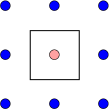
Figure 6: A plaquette on the original lattice corresponds to a Peierls domain wall on the dual lattice, separating the site at its center with reversed spin from the outside.

To illustrate this, the internal energy $U$ is computed, using the plaquette update. On an infinite lattice, the Kramers-Wannier duality implies that observables calculated at an inverse temperature $\beta$ in the original Ising model can be transcribed to those of the dual model at an inverse temperature $\tilde{\beta}$. The relation between the two temperatures follows from noting that, an occupied HT bond represents a factor $v$, while a nearest neighbor pair on the dual lattice of unlike spin on each side of the HT bond carries a Boltzmann weight $\exp(-2\tilde{\beta})$, so that [37]

$$\tanh\beta={\rm e}^{-2\tilde{\beta}},$$ (38)

or $\sinh 2\beta=1/\sinh 2\tilde{\beta}$.

On a finite lattice with periodic boundary conditions, however, a mismatch arises because single HT graphs wrapping the (finite) lattice are not generated by the plaquette update–such graphs always come in pairs. The HT Monte Carlo study will therefore not exactly simulate the Ising model with periodic boundary conditions, at least not for small lattice sizes. (For larger lattices, single graphs wrapping the lattice become highly unlikely, so that their absence will not be noticed anymore, and the HT Monte Carlo simulation becomes increasingly more accurate.) In contrast, on the dual side, where the plaquette update corresponds to a single spin update, this class of graphs is not compatible with the periodic boundary conditions, so that they should not be included. Hence, the plaquette update simulates the (transcribed) dual rather than the original model itself. Figure 7 gives the exact internal energy of the original Ising model on a finite lattice with periodic boundary conditions [39, 40] and that of the dual model transcribed to the original one using Eq. (38). In the figure, also the data points obtained using the plaquette update are included and seen to indeed coincide with the dual curve. For increasing lattice sizes, the dual and the original curves approach each other.

\psfrag{x}[t][t][.8][0]{$\beta$}\psfrag{y}[t][t][.8][0]{$U$}\psfrag{Ising}[c][t][.8][0]{Ising}\psfrag{MC}[c][t][.8][0]{MC}\psfrag{Dual}[c][t][.8][0]{Dual}\includegraphics[width=284.52756pt]{dual_update.eps}

Figure 7: Exact internal energy $U$ on a $16^{2}$ lattice for the Ising and dual model [transcribed to the original model using Eq. (38)], and the Monte Carlo data obtained using the plaquette update.

5.2 Simulation

To determine the graph proliferation temperature, the probability $P_{\rm S}$ for the presence of a graph spanning the lattice as function of $\beta$ is measured for different lattice sizes [4]. For small $\beta$, $P_{\rm S}$ tends to zero, while for large $\beta$ it tends to unity. We consider a graph spanning the lattice already when it does so in just one direction. Ideally, the curves obtained for different lattice sizes cross in a single point, marking the proliferation temperature. It is seen from Fig. 8 that within the achieved accuracy, the measured curves cross at the thermal critical point, implying that the HT graphs (domain walls) lose their line tension and proliferate precisely at the Curie point.

\psfrag{x}[t][t][.8][0]{$\beta/\beta_{\rm c}$}\psfrag{y}[t][t][.8][0]{$P_{\rm S}$}\psfrag{Ps16}[t][t][.8][0]{$16$}\psfrag{Ps32}[t][t][.8][0]{$32$}\psfrag{Ps64}[t][t][.8][0]{$64$}\psfrag{Ps128}[t][t][.8][0]{$128$}\psfrag{Ps256}[t][t][.8][0]{$256$}\includegraphics[width=284.52756pt]{cross.eps}

Figure 8: Probability $P_{\rm S}$ for the presence of a spanning graph as function of $\beta$ measured for different lattice sizes $L$. Within the achieved accuracy, the curves cross at the thermal critical point $\beta=\beta_{\rm c}$.

The data was collected in $3.3\times 10^{5}$ Monte Carlo sweeps of the lattice close to the critical point and $1.1\times 10^{5}$ outside the critical region, with about 10% of the sweeps used for equilibration. After each sweep, the resulting graph configuration was analyzed. Statistical errors were estimated by means of binning.

Finite-size scaling [4] predicts that the raw $P_{\rm S}$ data obtained for different lattice sizes collapse onto a single curve when plotted as function of $(\beta/\beta_{\rm c}-1)L^{1/\nu}$ with the right choice of the exponent $\nu$. By duality, the relevant correlation length here is that of the Ising model, so that $\nu$ takes the Ising value $\nu=1$. With this choice, a satisfying collapse of the data is achieved over the entire temperature range (see Fig. 9).

\psfrag{x}[t][t][.8][0]{$(\beta/\beta_{\rm c}-1)L^{1/\nu}$}\psfrag{y}[t][t][.8][0]{$P_{\rm S}$}\psfrag{Ps16}[t][t][.8][0]{$16$}\psfrag{Ps32}[t][t][.8][0]{$32$}\psfrag{Ps64}[t][t][.8][0]{$64$}\psfrag{Ps128}[t][t][.8][0]{$128$}\psfrag{Ps256}[t][t][.8][0]{$256$}\includegraphics[width=284.52756pt]{Ps_collapse.eps}

Figure 9: The raw data of Fig. 8 replotted as function of $(\beta/\beta_{\rm c}-1)L^{1/\nu}$, with the Ising choice $\nu=1$. The data collapse is satisfactory over the entire temperature range.

Next, the cluster exponents $\sigma_{\rm G}$ and $\tau_{\rm G}$ specifying the graph distribution,

$$\ell_{b}\sim b^{-\tau_{\rm G}}{\rm e}^{-\theta b},\quad\theta\propto(\beta-\beta_{\rm c})^{1/\sigma_{\rm G}}$$ (39)

are determined, where $\ell_{b}$ denotes the average number density of graphs containing $b$ bonds. To this end we measure the so-called percolation strength $P_{\infty}$, giving the fraction of bonds in the largest graph, and as second independent observable the average graph size [4] (see Fig. 10)

$$\chi_{\mathrm{G}}=\frac{\sum_{b}^{\prime}b^{2}\ell_{b}}{\sum_{b}^{\prime}b\ell_{b}},$$ (40)

where the prime on the sum indicates that the largest graph in each measurement is omitted.

\psfrag{x}[t][t][.8][0]{$\beta/\beta_{\mathrm{c}}$}\psfrag{y}[t][t][.8][0]{$P_{\infty}$}\psfrag{16}[t][t][.8][0]{$16$}\psfrag{32}[t][t][.8][0]{$32$}\psfrag{64}[t][t][.8][0]{$64$}\psfrag{128}[t][t][.8][0]{$128$}\psfrag{256}[t][t][.8][0]{$256$}\includegraphics[width=284.52756pt]{Po.eps}

\psfrag{x}[t][t][.8][0]{$\beta/\beta_{\mathrm{c}}$}\psfrag{y}[t][t][.8][0]{$P_{\infty}$}\psfrag{16}[t][t][.8][0]{$16$}\psfrag{32}[t][t][.8][0]{$32$}\psfrag{64}[t][t][.8][0]{$64$}\psfrag{128}[t][t][.8][0]{$128$}\psfrag{256}[t][t][.8][0]{$256$}\psfrag{x}[t][t][.8][0]{$\beta/\beta_{\mathrm{c}}$}\psfrag{y}[t][t][.8][0]{$\chi_{\mathrm{G}}$}\includegraphics[width=284.52756pt]{chi.eps}

Figure 10: The percolation strength $P_{\infty}$ (top panel) and average graph size $\chi_{\mathrm{G}}$ (bottom panel) as function of $\beta/\beta_{\mathrm{c}}$ for different lattice sizes $L$.

Close to the proliferation temperature, these observables obey the finite-size scaling relations [41]

$$P_{\infty}=L^{-\beta_{\rm G}/\nu}\,{\sf P}(L/\xi),\quad\chi_{\mathrm{G}}=L^{\gamma_{\rm G}/\nu}\,{\sf X}(L/\xi),$$ (41)

where $\xi$ is the correlation length and the critical exponents $\beta_{\rm G},\gamma_{\rm G}$ are related to $\sigma_{\rm G},\tau_{\rm G}$ through Eq. (3.1) written in terms of the variables appropriate for the graph exponents. Precisely at $T_{\rm c}$, these scaling relations imply an algebraic dependence on the system size $L$, allowing for a determination of the exponent ratios (see Table 2 and Fig. 11).

\psfrag{x}[t][t][.8][0]{$L$}\psfrag{y}[t][t][.8][0]{$P_{\infty}$}\psfrag{f}[t][t][.8][0]{}\includegraphics[width=284.52756pt]{Po_fit.eps}

\psfrag{x}[t][t][.8][0]{$L$}\psfrag{y}[t][t][.8][0]{$P_{\infty}$}\psfrag{f}[t][t][.8][0]{}\psfrag{x}[t][t][.8][0]{$L$}\psfrag{y}[t][t][.8][0]{$\chi_{\mathrm{G}}$}\psfrag{f}[t][t][.8][0]{}\includegraphics[width=284.52756pt]{chi_fit.eps}

Figure 11: Log-log plot of the percolation strength $P_{\infty}$ (top panel) and average graph size $\chi_{\mathrm{G}}$ (bottom panel) at the critical temperature as function of the lattice size $L$. The straight lines $0.642\,L^{-0.626}$ and $1.139\,L^{0.740}$, respectively are obtained through two-parameter fits.

Table 2: Percolation strength $P_{\infty}$ and average graph size $\chi_{\mathrm{C}}$ at the (inverse) critical temperature $\beta_{\rm c}=\ln(1+\sqrt{2})/2=0.440687\cdots$ for various lattice sizes $L$ (see Fig. 11).

$L$	16	20	24	32	40	48	64	80	96	128
$P_{\infty}$	0.1129(6)	0.0986(7)	0.0876(6)	0.0744(7)	0.0642(8)	0.0569(8)	0.0461(9)	0.0426(11)	0.0353(10)	0.0312(12)
$\chi_{\mathrm{C}}$	8.90(4)	10.44(4)	11.91(5)	14.86(8)	17.44(10)	20.03(16)	24.55(22)	29.61(34)	33.13(39)	41.93(81)

The data was fitted using the nonlinear least-squares Marquardt-Levenberg algorithm, giving

$$\beta_{\rm G}=0.626(7)\quad\gamma_{\rm G}=0.740(4),$$ (42)

with $\chi^{2}/{\rm d.o.f}=1.15$ and $0.94$, respectively, and where it was used that $\nu=1$. These values are perfectly consistent with the fractions $\beta_{\rm G}=\frac{5}{8}=0.625,\gamma_{\rm G}=\frac{3}{4}=0.75$, leading to the exponents

$$\sigma_{\rm G}=\frac{8}{11},\quad\tau_{\rm G}=\frac{27}{11},$$ (43)

and the fractal dimension

$$D_{\rm H}^{\rm G}=\frac{11}{8}$$ (44)

of the HT graphs we were seeking. By duality, this fractal dimension equals that of the hull bounding the geometrical spin clusters (Peierls domain walls) on the dual lattice. Our numerical result agrees with Eq. (29b) with $\bar{\kappa}=\bar{\kappa}_{\rm Ising}=\frac{4}{3}$ appropriate for the Ising model.

The value (44) was predicted by Duplantier and Saleur, using the Coulomb gas map [25]. Subsequent support for that prediction was provided by Vanderzande and Stella [20] who drew on earlier numerical work by Cambier and Nauenberg [42]. A first direct numerical determination was given by Dotsenko et al. [43]. Employing the Swendsen-Wang cluster update, these authors analyzed the geometrical spin clusters and their hulls at the critical temperature. They extracted the fractal dimension from the resulting hull distribution, which is algebraic at the critical temperature. Apart from directly simulating the hulls with the plaquette update, another advantage of our approach is the use of finite-size scaling which is generally considered more reliable than the extraction of exponents by fits to the data obtained for a fixed lattice size.

As argued in Sec. 4 for the general case, the geometrical Ising clusters correspond to the tricritical Potts model with $\bar{\kappa}=\bar{\kappa}_{-}=1/\bar{\kappa}_{\rm Ising}=\frac{3}{4}$, which according to Eq. (32) is the tricritical $q=1$ model [19]. In addition to the correlation length exponent $\nu=1$ which we, in accordance with Eq. (33), observed numerically and the second thermal eigenvalue $y_{T}^{\mathrm{G}}=\frac{15}{8}$, this tricritical behavior is further characterized by [12] $\beta_{\mathrm{C}}=\frac{5}{96}$. This value follows from the scaling relation (25) with the fractal dimension $D_{\mathrm{C}}$ of the FK clusters replaced by that of their geometrical counterpart (29a) with $\bar{\kappa}=\bar{\kappa}_{\rm Ising}=\frac{4}{3}$ [19].

The fact that the two correlation length exponents featuring in the critical $q=2$ and tricritical $q=1$ Potts models are equal is special to this case, being a result of the Kramers-Wannier duality. Indeed, equating the correlation length exponent (12) of the critical Potts models and that of the tricritical Potts models given in (33) with $\bar{\kappa}_{-}=1/\bar{\kappa}$ to assure that both models have the same central charge, yields $\bar{\kappa}=\bar{\kappa}_{\rm Ising}=\frac{4}{3}$ as only physical solution.

6 Summary

In this paper, it is shown that the geometrical spin clusters of the pure $q$-state Potts model in two dimensions encode the tricritical behavior of the site diluted model. These clusters, formed by nearest neighbor sites of like spins, were shown to be mirror images of FK clusters, which in turn encode the critical behavior. Since the mirror map conserves the central charge, both cluster types (and thus both fixed points) are in the same universality class. The geometrical picture was supported by a Monte Carlo simulation of the high-temperature representation of the Ising model, corresponding to $q=2$. The use of a plaquette update allowed us to directly simulate the hulls of the geometrical clusters and to accurately determine their fractal dimension.

References

- [1] R. B. Potts, Proc. Camb. Phil. Soc. 48, 106 (1952).
- [2] C. M. Fortuin and P. W. Kasteleyn, Physica 57, 536 (1972).
- [3] F. Y. Wu, Rev. Mod. Phys. 54, 235 (1982).
- [4] D. Stauffer and A. Aharony, Introduction to Percolation Theory, 2nd edition (Taylor & Francis, London, 1994).
- [5] R. H. Swendsen and J. S. Wang, Phys. Rev. Lett. 58, 86 (1987).
- [6] U. Wolff, Phys. Rev. Lett. 62, 361 (1989).
- [7] R. J. Baxter, J. Phys. C 6, L445 (1973).
- [8] B. Nienhuis, A. N. Berker, E. K. Riedel, and M. Schick, Phys. Rev. Lett. 43, 737 (1979).
- [9] O. Schramm, Israel J. Math., 118, 221 (2000).
- [10] The parameter we use is related to the label in Ref. [9] through . The reason for our convention will become clear when we proceed [see, e.g., Eq. (28)].
- [11] M. P. M. den Nijs, J. Phys. A 12, 1857 (1979); Phys. Rev. B 27, 1674 (1983).
- [12] B. Nienhuis, J. Phys. A 15, 199 (1982); in: Phase Transitions and Critical Phenomena, edited by C. Domb and J. L. Lebowitz (Academic, London, 1987), Vol. 11, p.1.
- [13] H. Saleur and B. Duplantier, Phys. Rev. Lett. 58, 2325 (1987).
- [14] J. Cardy, in: Phase Transitions and Critical Phenomena, edited by C. Domb and J. L. Lebowitz (Academic, London, 1987), Vol. 11, p.55
- [15] B. Duplantier, J. Stat. Phys. 110, 691 (2003).
- [16] S. Rohde and O. Schramm, Basic properties of SLE, Ann. Math. (to appear), math.PR/0106036 (2001).
- [17] M. Bauer and D. Bernard, Commun. Math. Phys. 239, 493 (2003).
- [18] B. Duplantier, Conformal Fractal Geometry and Boundary Quantum Gravity, math-ph/0303034 (2003).
- [19] A. L. Stella and C. Vanderzande, Phys. Rev. Lett. 62, 1067 (1989).
- [20] C. Vanderzande and A. L. Stella, J. Phys. A 22, L445 (1989).
- [21] T. Temesvári and L. Herényi, J. Phys. A 17, 1703 (1984).
- [22] A. Coniglio and W. Klein, J. Phys. A 13, 2775 (1980).
- [23] B. Duplantier, J. Stat. Phys. 49, 411 (1987).
- [24] H.-M. Erkinger, A new cluster algorithm for the Ising model, Diplomarbeit, Technische Universität Graz (2000).
- [25] B. Duplantier and H. Saleur, Phys. Rev. Lett. 61, 1521 (1988).
- [26] K. K. Murata, J. Phys. A 12, 81 (1979).
- [27] C. Vanderzande, J. Phys. A 25, L75 (1992). A typo seems to be present in the right hand of Eq. (10) of that paper, giving the fractal dimension of the red bonds of the geometrical clusters. It should read , where is related to through Eq. (16). The corresponding entries in Table 1 of that paper should be updated accordingly.
- [28] A. M. J. Schakel, Phys. Rev. E 63, 026115 (2001); J. Low Temp. Phys 129, 323 (2002).
- [29] A. Coniglio, Phys. Rev. Lett. 62, 3054 (1989).
- [30] B. Duplantier, Phys. Rev. Lett. 84, 1363 (2000).
- [31] T. Grossman and A. Aharony J. Phys. A 19, L745 (1986); 20, L1193 (1987).
- [32] M. Aizenman, B. Duplantier, and A. Aharony, Phys. Rev. Lett. 83, 1359 (1999).
- [33] J. Asikainen, A. Aharony, B. B. Mandelbrot, E. M. Rauch, and J.-P. Hovi, Eur. Phys. J. B 34, 479 (2003).
- [34] H. E. Stanley, J. Phys. A 10, L211 (1977).
- [35] B. Duplantier and H. Saleur, Phys. Rev. Lett. 63, 2536 (1989).
- [36] R. P. Feynman, Statistical Mechanics (Benjamin, Reading, 1972).
- [37] H. A. Kramers and G. H. Wannier, Phys. Rev. 60, 252 (1941).
- [38] R. Peierls, Proc. Camb. Phil. Soc. 32, 477 (1936).
- [39] B. Kaufman, Phys. Rev. 76, 1232 (1949); A. E. Ferdinand and M. E. Fisher, Phys. Rev. 185, 832 (1969).
- [40] W. Janke, Monte Carlo Simulations of Spin Systems, in: Computational Physics: Selected Methods – Simple Exercises – Serious Applications, edited by K. H. Hoffmann and M. Schreiber (Springer, Berlin, 1996); p. 10.
- [41] K. Binder and D. W. Heermann, Monte Carlo Simulation in Statistical Physics (Springer, Berlin, 1997).
- [42] J. L. Cambier and M. Nauenberg, Phys. Rev. B 34, 8071 (1986).
- [43] V. S. Dotsenko, M. Picco, P. Windey, G. Harris, E. Martinec, and E. Marinari, Nucl. Phys. B 448 [FS], 577 (1995).