Cluster Monte Carlo algorithms

1 Introduction

In recent years, a better understanding of the Monte Carlo method has provided us with many new techniques in different areas of statistical physics. Of particular interest are so called cluster methods, which exploit the considerable algorithmic freedom given by the detailed balance condition. Cluster algorithms appear, among other systems, in classical spin models, such as the Ising model [1], in lattice quantum models (bosons, quantum spins and related systems) [2] and in hard spheres and other ‘entropic’ systems for which the configurational energy is either zero or infinite [3].

In this chapter, we discuss the basic idea of cluster algorithms with special emphasis on the pivot cluster method for hard spheres and related systems, for which several recent applications are presented. We provide less technical detail but more context than in the original papers. The best implementations of the pivot cluster algorithm, the ‘pocket’ algorithm [4], can be programmed in a few lines. We start with a short exposition of the detailed balance condition, and of ‘a priori’ probabilities, which are needed to understand how optimized Monte Carlo algorithms may be developed. A more detailed discussion of these subjects will appear in a forthcoming book [5].

2 Detailed balance and a priori probabilities

In contrast with the combinatorial optimization methods discussed elsewhere in this book, the Monte Carlo approach does not construct a well-defined state of the system —minimizing the energy, or maximizing flow, etc—but attempts to generate number of statistically independent representative configurations $a$, with probability $\pi(a)$. In classical equilibrium statistical physics, $\pi(a)$ is given by the Boltzmann distribution, whereas, in quantum statistics, the weight is the diagonal many-body density matrix.

In order to generate these configurations with the appropriate weight (and optimal speed), the Monte Carlo algorithm moves (in one iteration) from configuration $a$ to configuration $b$ with probability $P(a\rightarrow b)$. This transition probability is chosen to satisfy the fundamental condition of detailed balance

$$\pi(a)P(a\rightarrow b)=\pi(b)P(b\rightarrow a)$$ (1)

which is implemented using the Metropolis algorithm

$$P(a\rightarrow b)=\min\left(1,\frac{\pi(b)}{\pi(a)}\right)$$ (2)

or one of its variants.

For the prototypical Ising model, the stationary probability distribution (the statistical weight) of a configuration is the Boltzmann distribution with an energy given by

$$E=-J\sum_{\langle i,j\rangle}S_{i}S_{j}\quad L>0$$ (3)

as used and modified in many other places in this book. A common move consists of a spin flip on a particular site $i$, transforming configuration $a$ into another configuration $b$. This is shown in Fig. 1 (left). In a hard sphere gas, also shown in Fig. 1 (right), one typically displaces a single particle $i$ from $\mathbf{x}$ to $\mathbf{x}+\boldsymbol{\delta}$. There is a slight difference between these two simple algorithms: by flipping the same spin twice, one goes back to the initial configuration: a spin flip is its own inverse. In contrast, in the case of the hard-sphere system, displacing a particle twice by the same vector $\boldsymbol{\delta}$ does not usually bring one back to the original configuration.

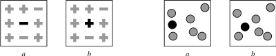
Figure 1: Two examples of local Monte Carlo algorithms: the two-dimensional Ising model with single-spin flip dynamics (left) and two-dimensional hard disks with a single-particle move (right).

An essential concept is the one of an a priori probability: it accounts for the fact that the probability $P(a\rightarrow b)$ is a composite object, constructed from the probability of considering the move from $a$ to $b$, and the probability of accepting it.

$$P(a\rightarrow b)=\underbrace{\mathcal{A}(a\rightarrow b)}_{\text{consider}\ a\rightarrow b}\times\underbrace{\tilde{P}(a\rightarrow b)}_{\text{accept}\ a\rightarrow b}$$

In usual Monte Carlo terminology, if $a\rightarrow b$ is rejected (after having been considered), then the ‘move’ $a\rightarrow a$ is chosen instead and the system remains where it is.

With these definitions, the detailed balance condition eq. (1) can be written as

$$\frac{\tilde{P}(a\rightarrow b)}{\tilde{P}(b\rightarrow a)}=\frac{\pi(b)}{\mathcal{A}(a\rightarrow b)}\frac{\mathcal{A}(b\rightarrow a)}{\pi(a)}$$

and implemented by a Metropolis algorithm generalized from eq. (2):

$$\tilde{P}(a\rightarrow b)=\min\left\{1,\frac{\pi(b)}{\mathcal{A}(a\rightarrow b)}\frac{\mathcal{A}(b\rightarrow a)}{\pi(a)}\right\}$$ (4)

It is very important to realize that the expression “a priori probability $\mathcal{A}(a\rightarrow b)$” is synonymous to “Monte Carlo algorithm”. A Monte Carlo algorithm $\mathcal{A}(a\rightarrow b)$ of our own conception must satisfy three conditions:

1. It must lead the state of the system from a configuration $a$ to a configuration $b$, in such a way that, eventually, all configurations in phase space can be reached (ergodicity).

2. It must allow to compute the ratio $\pi(a)/\pi(b)$. This is trivially satisfied, at least for classical systems, as the statistical weight is simply a function of the energy.

3. It must allow, for any possible transition $a\rightarrow b$, to compute both the probabilities $\mathcal{A}(a\rightarrow b)$ and $\mathcal{A}(b\rightarrow a)$. Again, it is the ratio of probabilities which is important.

A trivial application of a priori probabilities for hard spheres is given in Fig. 2. (Suppose that the points $a$ and $b$ are embedded in a large two-dimensional plane.) On the left side of the figure, we see one of the standard choices for the trial moves $\mathbf{x}\rightarrow\mathbf{x}+\boldsymbol{\delta}$ of a particle in Fig. 1: The vector $\boldsymbol{\delta}$ is uniformly sampled from a square centered around the current position. If however, we decide, for some obscure reason, to sample $\boldsymbol{\delta}$ from a triangle, we realize that in cases such the one shown in Fig. 2 (right), the a priori probability for the return move vanishes. It is easy to see from eq. (4) that, in this case, both $P(a\rightarrow b)$ and $P(b\rightarrow a)$ are zero.

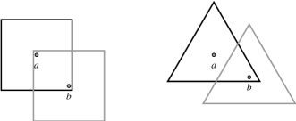
Figure 2: A priori probabilities for the hard-sphere system. Left: ‘square’—$\mathcal{A}(a\rightarrow b)$ is constant within the square boundary, and zero outside. By construction, $\mathcal{A}(a\rightarrow b)=\mathcal{A}(b\rightarrow a)$. Right: ‘triangle’—for the analogous (if hypothetical) case of a triangle, there are pairs $a,b$, where $\mathcal{A}(a\rightarrow b)$ is finite, but $\mathcal{A}(b\rightarrow a)=0$. Both rates $P(a\rightarrow b)$ and $P(b\rightarrow a)$ vanish.

Notwithstanding its simplicity, the triangle ‘algorithm’ illustrates that any Monte Carlo method $\mathcal{A}(a\rightarrow b)$ can be made to comply with detailed balance, if we feed it through eq. (4). The usefulness of the algorithm is uniquely determined by the speed with which it moves through configuration space, and is highest if no rejections at all appear. It is to be noted however that, even if $\tilde{P}(a\rightarrow b)$ is always $1$ (no rejections), the simulation can remain rather difficult. This happens for example in the two-dimensional $XY$-model and in several examples treated below.

Local algorithms are satisfactory for many problems but fail whenever the typical differences between relevant configurations are much larger than the change that can be achieved by one iteration of the Monte Carlo algorithm. In the Ising model at the critical point, for example, the distribution of magnetizations is wide, but the local Monte Carlo algorithm implements a change of magnetization of only $\pm 2$. This mismatch lies at the core of critical slowing down in experimental systems and on the computer.

In liquids, modeled e.g. by the hard-sphere system, another well-known limiting factor is that density fluctuations can relax only through local diffusion. This process generates slow hydrodynamic modes, if the overall diffusion constants are small.

Besides these slow dense systems, there is also the class of highly constrained models, of which binary mixtures will be treated later. In these systems, the motion of some degrees of freedom naturally couple to many others. In a binary mixture, e. g., a big colloidal particle is surrounded by a large number of small particles, which are influenced by its motion. This is extremely difficult to deal with in Monte Carlo simulations, where the local moves $\mathbf{x}\rightarrow\mathbf{x}+\boldsymbol{\delta}$ are essentially the unconstrained motion of an isolated particle.

3 The Wolff cluster algorithm for the Ising model

The local spin-flip Monte Carlo algorithm not being satisfactory, it would be much better to move large parts of the system, so called clusters. This cannot be done by a blind flip of one or many spins (with $\mathcal{A}(a\rightarrow b)=\mathcal{A}(b\rightarrow a)$), which allows unit acceptance rate both for the move $a\rightarrow b$ and its reverse $b\rightarrow a$ only if the energies of both configurations are the same. One needs an algorithm whose a priori probabilities ${\mathcal{A}}(a\rightarrow b)$ and ${\mathcal{A}}(b\rightarrow a)$ soak up any differences in statistical weight $\pi(a)$ and $\pi(b)$.

This can be done by starting the construction of a cluster with a randomly sampled spin and by iteratively adding neighboring sites of the same magnetization with a probability $p$. To be precise, one should speak about ‘links’: if site $i$ is in the cluster and a neighboring site $j$ is not, and if, furthermore, $S_{i}=S_{j}$, then one should add link $\langle i,j\rangle$ with probability $p$. A site is added to the cluster if it is connected by at least one link. In configuration $a$ of Fig. 3, the cluster construction has stopped in the presence of $9$ links “$--$” across the boundary. Each of these links could have been accepted with probability $p$, but has been rejected. This gives a term $(1-p)^{9}$ in the a priori probability. Flipping the cluster brings us to configuration $b$. The construction of the cluster for configuration $b$ would stop in the presence of $19$ links “$++$” across the boundary (a priori probability $\propto(1-p)^{19}$)).

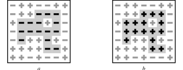
Figure 3: The Wolff cluster algorithm for the Ising model adds, with probability $p$, a link connecting a site outside the cluster to a site already in the cluster (thereby adding the site). In the configuration $a$, construction of the cluster (as shown) stopped with $9$ links “$--$”, corresponding to an a priori probability $\mathcal{A}(a\rightarrow b)=\mathcal{A}_{\text{interior}}\times(1-p)^{9}$. The return move stops with probability $\mathcal{A}(b\rightarrow a)=\mathcal{A}_{\text{interior}}\times(1-p)^{19}$, as there are $19$ links “$++$” across the boundary in configuration $b$.

This allows us to compute the a priori probabilities

$$\mathcal{A}(a\rightarrow b) =\mathcal{A}_{\text{interior}}\times(1-p)^{9}$$

$$\mathcal{A}(b\rightarrow a) =\mathcal{A}_{\text{interior}}\times(1-p)^{19}$$

$$E_{a} =E_{\text{interior}}+E_{\text{exterior}}-9\times J+19\times J (\pi_{a}=\exp[-\beta E_{a}])$$

$$E_{b} =E_{\text{interior}}+E_{\text{exterior}}-19\times J+9\times J (\pi_{b}=\exp[-\beta E_{b}])$$

In these equations, the ‘interior’ refers to the part of the cluster which does not touch the boundary. By construction, the ‘interior’ and ‘exterior’ energies and a priori probabilities are the same for any pair of configurations $a$ and $b$ which are connected through a single cluster flip.

We thus dispose of all the information needed to evaluate the acceptance probability $\tilde{P}$ in eq. (4), which we write more generally in terms of the number of “same” and of “different” links in the configuration $a$. These notions are interchanged for configuration $b$ (in Fig. 3, we have $n_{\text{same}}=9$, $n_{\text{diff}}=19$). With the energy scale $J$ set to $1$, we find

$$\tilde{P}(a\rightarrow b) =\min\left\{1,\frac{e^{\beta n_{\text{diff}}}e^{-\beta n_{\text{same}}}}{(1-p)^{n_{\text{same}}}}\frac{(1-p)^{n_{\text{diff}}}}{e^{-\beta n_{\text{diff}}}e^{\beta n_{\text{same}}}}\right\}$$

$$=\min\left\{1,\left[\frac{e^{-2\beta}}{1-p}\right]^{n_{\text{same}}}\left[\frac{1-p}{e^{-2\beta}}\right]^{n_{\text{diff}}}\right\}$$ (5)

Once the cluster construction stops, we know the configuration $b$, may count $n_{\text{same}}$ and $n_{\text{diff}}$, and evaluate $\tilde{P}(a\rightarrow b)$. Of course, a lucky coincidence occurs for $p=1-\exp[-2J\beta]$. This special choice yields a rejection-free algorithm whose acceptance probability is unity for all possible moves and is implemented in the celebrated Wolff cluster algorithm [1], the fastest currently known simulation method for the Ising model. The Wolff algorithm can be programmed in a few lines, by keeping a vector of cluster spins, and an active frontier, as shown below. The algorithm below presents a single iteration $a\rightarrow b$. The function $\text{ran}[0,1]$ denotes a uniformly distributed random number between $0$ and $1$, and $p$ is set to the magical value $p=1-\exp[-2J\beta]$. The implementation uses the fact that a cluster can grow only at its frontier (called the ‘old’ frontier $\mathcal{F}_{\text{old}}$, and generating the new one $\mathcal{F}_{\text{new}}$). It goes without saying that for the magic value of $p$ we do not have to evaluate $\tilde{P}(a\rightarrow b)$ in eq. (5), as it is always $1$. Any proposed move is accepted.

algorithm wolff-cluster
begin
	$i:=\text{random particle}$;
	$\mathcal{C}:=\{i\}$;
	$\mathcal{F}_{\text{old}}:=\{i\};$
	while $\mathcal{F}_{\text{old}}\neq\{\}$ do
	begin
		$\mathcal{F}_{\text{new}}:=\{\};$
		for $\forall\ i\ \in\ \mathcal{F}_{\text{old}}$ do
		begin
			for $\forall\ j\ \text{neighbor of $i$ with $S_{i}=S_{j}$},\ j\not\in\mathcal{C}$ do
			begin
				if $\text{ran}[0,1]<p$ then
				begin
					$\mathcal{F}_{\text{new}}:=\mathcal{F}_{\text{new}}\cup\{j\};$
					$\mathcal{C}:=\mathcal{C}\cup\{j\};$
				end
			end
		end
		$\mathcal{F}_{\text{old}}:=\mathcal{F}_{\text{new}};$
	end
	for $\forall\ i\ \in\ \mathcal{C}$ do
	$S_{i}:=-S_{i};$
end

4 Cluster algorithm for hard spheres and related systems

We want to further exploit the analogy between the spin model and the hard-sphere system. As the spin-cluster algorithm constructs a cluster of spins which flip together, one might think that a cluster algorithm for hard spheres should identify ‘blobs’ of spheres that move together. Such a macroscopic ballistic motion would replace slow diffusion.

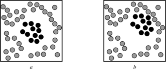
Figure 4: The dark disks are easier to identify as a cluster in configuration $a$ than in $b$, where they are fused into the background. This means that, for the configurations $a$ and $b$ shown in this figure, $\mathcal{A}(a\rightarrow b)\gg\mathcal{A}(b\rightarrow a)$ for any generic Monte Carlo algorithm. As $\pi(a)=\pi(b)$, the acceptance probability $\tilde{\mathcal{P}}(a\rightarrow b)$ in eq. (4) will be extremely small. The problem can be avoided [3] if the transformation $a\rightarrow b$ is protected by a symmetry principle: it must be its own inverse.

To see that this strategy cannot be successful, it suffices to look at the generalized detailed balance condition in the example shown in Fig. 4: any reasonable algorithm $\mathcal{A}$ would have less trouble spotting the cluster of dark disks in configuration $a$ than in $b$. This means that $\mathcal{A}(a\rightarrow b)\gg\mathcal{A}(b\rightarrow a)$ and that the acceptance rate $\tilde{P}(a\rightarrow b)$ would be very small.

The imbalance between $\mathcal{A}(a\rightarrow b)$ and $\mathcal{A}(b\rightarrow a)$ can however be avoided if the two transition probabilities are protected by a symmetry principle: the transformation $T$ producing $b$ from $a$ must be the same as the one producing $a$ from $b$. Thus, $T$ should be its own inverse.

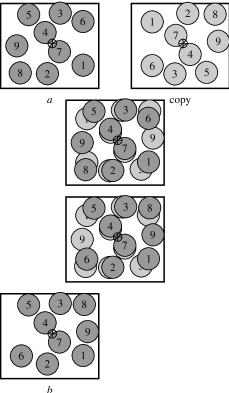
Figure 5: The pivot cluster algorithm performs a symmetry operation which is its own inverse. In this system of hard disks (with periodic boundary conditions), a rotation by an angle $\pi$ around an arbitrarily sampled pivot ($\oplus$) is shown: $a$ is the original configuration, $b$ the rotated copy. The intermediate pictures show the superposed system of original and copy before and after the flip. The final configuration, $b$, is also shown. Notice that the transformation maps the simulation box (with periodic boundary conditions) onto itself. If this is not the case, the treatment of boundary conditions becomes more involved, and generates rejections.

In Fig. 5, this program is applied to a hard disk configuration using as transformation $T$ a rotation by an angle $\pi$ around an arbitrarily sampled pivot (denoted by $\oplus$, for each iteration a new pivot is used). Notice that for a symmetric particle, the rotation by an angle $\pi$ is identical to the reflection around the pivot. It is useful to transform not just a single particle, but the whole original configuration $a$ yielding the ‘copy’. By overlaying the original with its rotated copy, we may identify the invariant sub-ensembles (clusters) which transform independently under $T$. For example, in Fig. 5, we may rotate the disks numbered $6$, $8$, and $9$, which form a cluster of overlapping disks in the ensemble of overlayed original and copy.

In Fig. 5, there are the following three invariant clusters:

$$\{6,8,9\},\{2,3,4,7\},\{1,5\}$$ (6)

The configuration $b$ in Fig. 5 shows the final positions positions after rotation of the first of these clusters. By construction, $\mathcal{A}(a\rightarrow b)=\mathcal{A}(b\rightarrow a)$ and $\pi(a)=\pi(b)$. This perfect symmetry ensures that detailed balance is satisfied for the non-local move. Notice that moving the cluster $\{1,5\}$ is equivalent to exchanging the labels of the two particles and performing two local moves. Ergodicity of the algorithm follows from ergodicity of the local algorithm, as a local move $\mathbf{x}\rightarrow\mathbf{x}+\boldsymbol{\delta}$ can always be disguised as a cluster rotation around the pivot $\mathbf{x}+\boldsymbol{\delta}/2$.

Fig. 5 allows to understand the basic limitation of the pivot cluster approach: if the density of particles becomes too large, almost all particles will be in the same cluster, and flipping it will essentially rotate the whole system. Nevertheless, even though above the percolation threshold in the thermodynamic limit there exists a large cluster containing a finite fraction of all particles, the distribution of small clusters obeys an algebraic decay law. This means that finite clusters of various sizes will be produced. These may give rise to useful moves, for example in the case of dense polydisperse disks discussed farther below. Even small clusters provide non-diffusive mass transport if they contain an odd number of particles (cf. the example in Fig. 5) or particles of different type.

It is also useful to discuss what will happen if the “copy” does not stem from a symmetry operation, for example if the copy is obtained from the original through a simple translation with a vector $\boldsymbol{\delta}$. In this case, there would still be clusters, but they no longer appear in pairs. It would still be possible to flip individual clusters, but not to conserve the number of particles on each plate. This setting can also have important applications, it is very closely related to Gibbs ensemble simulations and provides an optimal way of exchanging particles between two plates. The two plates would no longer describe the same system but be part of a larger system of coupled plates.

algorithm pocket-cluster
begin
	$\mathbf{r}_{\text{pivot}}:=\text{random point in box}$;
	$i:=\text{random particle}$;
	$\mathcal{P}:=\{i\}$;
	$\mathcal{O}:=\{\text{all particles}\}\setminus\{i\}$;
	while $\mathcal{P}\neq\{\}$ do
	begin
		$i:=\text{any element of}\ \mathcal{P}$;
		$\mathcal{P}:=\mathcal{P}\setminus\{i\}$;
		$\mathbf{r}(i):=\text{reflection of $\mathbf{r}(i)$ around $\mathbf{r}_{\text{pivot}}$}$;
		for $\forall\ j\ \in\ \mathcal{O}$ do
		if $j\ \cap\ i$ then
		begin
			$\mathcal{O}:=\mathcal{O}\setminus\{j\}$;
			$\mathcal{P}:=\mathcal{P}\cup\{j\}$;
		end
	end
end

Having discussed the conceptual underpinnings of the pivot cluster algorithm, it is interesting to understand how it can be made into a working program. Fig. 5 suggests one should use a representation with two plates, and perform cluster analyses, very similar to what is done in the Wolff algorithm.

However, it is not necessary to work with two plates: The transformation can be done on the system itself and does not even have to consider a cluster at all. This ultimately simple solution is achieved in the ‘pocket’ algorithm [4]: it merely keeps track of particles which eventually have to be moved in order to satisfy all the hard-core constraints: After sampling the pivot (or another symmetry operation), one chooses a first particles, which is put into the pocket. In each stage of the iteration, one particle is taken from the pocket, and the transformation is applied to it. At the particle’s new position, the hard-core constraint will probably be violated for other particles. These have simply to be marked as ‘belonging to the pocket’. One single ‘move’ of the cluster algorithm consists in all the stages until the pocket is empty or, equivalently, in all the steps leading from frame $a$ to frame $e$ in Fig. 6. The inherent symmetry guarantees that the process will end with an empty pocket, and detailed balance will again be satisfied as the output is the same as in the two-plate version.

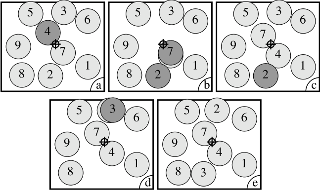
Figure 6: One iteration of the pocket algorithm (‘pocket’ $\equiv$ ‘dark disks’). Initially (frame $a$), a pivot is chosen and a starting disk (here disk $4$) is put into the pocket. At each subsequent step, a disk is removed from the pocket and transformed with respect to the pivot. Any overlapping disks are added to the pocket. For example, in frame $b$, overlaps exist between disk $4$ (which has just been moved) and disks $2$ and $7$. Only one of these disks is transformed in frame $c$. The pocket algorithm is guaranteed to move from valid hard-disk configuration to another one, and to respect detailed balance. It can be implemented in a few lines of code, as shown below.

In the printed algorithm, $\mathcal{P}$ stands for the “pocket”, and $\mathcal{O}$ is the set of “other” particles that currently do not have to be moved to satisfy the hard-core constraints. The expression $j\cap i$ is ‘true’ if the pair $i,j$ violates the hard-core constraint.

5 Applications

Phase separation in binary mixtures

Figure 7: Entropic interaction between two colloids (squares of edge length $d_{\text{large}}$) in a sea of small particles (of size $d_{\text{small}}$). Left: Small particles cannot penetrate into the slit between the large particles. The concentration difference leads to an effective entropic interaction between colloids, which is attractive at small separation. Right: At large distances between colloids, the effective interaction vanishes.

The depletion force—one of the basic interactions between colloidal particles—is of purely entropic origin. It is easily understood for a system of large and small squares (or cubes): In the left picture of Fig. 7, the two large squares are very close together so that no small particles can penetrate into the slit between the large ones. The finite concentration of small squares close to the large squares constitutes a concentration (pressure) difference between the outside and the inside, and generates an osmotic force which pulls the large squares together. The model of hard oriented squares (or cubes) serves as an ‘Ising model of binary liquids’ [6], for which the force is very strong because of the large contact area between them. Besides this, the situation is qualitatively similar to the one for hard spheres.

For a long time, there was a dispute as to whether the depletion interaction (which is oscillatory—repulsive and attractive, starting with an attractive piece at small distances) was sufficiently strong to induce phase transitions. The situation has been cleared up recently due to experimental, analytical and numerical work.

We want to perform Monte Carlo simulation on this system [7, 8]. But as one can see immediately, this is not simple: While the small squares may move with a local algorithm of Fig. 1, the large particles suffer from a serious ‘pope in the crowd’ effect: The large square is surrounded by so many small particles in its immediate neighorhood that any trial move will somewhere lead to the violation of the hard-core constraint, i.e. it will be rejected. A local Monte Carlo algorithm has vanishing acceptance rate for the motion of the large particles in the limit of $d_{\text{small}}/d_{\text{large}}\rightarrow 0$, expressing the increasing number of constraints in this limit.

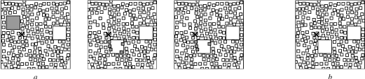
Figure 8: Pocket algorithm applied to the binary mixture of squares. The first three stages, and the final configuration of one step are shown. Note that the squares which are fully covered by the moved large square can be transformed immediately, without passing through the pocket, as they will not induce further overlaps.

The pivot cluster method provides a straightforward solution to this problem: randomly pick a square (large or small), and transform it by applying a symmetry operation of the whole system (rotation around a random pivot, reflection about a symmetry axis of the lattice). At each stage of the algorithm, pick an arbitrary particle from the pocket, transform it and add to the pocket any particles it may overlap with.

As can be seen in Fig. 8, there is a nice simplification: particles which are completely covered by a ‘big’ particle (as in the second frame of Fig. 8) will never generate new constraint violations. These particles can be transformed directly, without passing through the pocket.

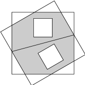
Figure 9: The figure shows a transformation (reflection about a straight line) which is not a symmetry transformation of the whole system (with periodic boundary conditions). In this case, cluster transformations involving squares outside the gray area have to be rejected. Transformations as the ones shown allow to reach arbitrary orientations of the squares.

Using this algorithm, it has become possible to directly show that binary mixtures undergo a phase separation transition, where the large particles crystallize. The transition takes place at smaller and smaller densities as the size mismatch $d_{\text{large}}/d_{\text{small}}$ increases at, say, constant ratio of densities. At the same time, the percolation threshold of the combined two-plate system is sensitive only to the total density of particles.

It is also possible to relax the ‘orientation’ constraint. This can be done with transformations $T$ which satisfy $T^{2}=1$, but are not symmetries of the simulation box. An example is shown in Fig. 9.

Polydisperse mixtures

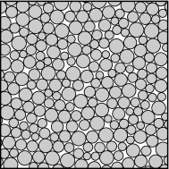
Figure 10: Dense configuration of polydisperse hard disks, for which the time evolution of a local Monte Carlo algorithm is immeasurably slow. The cluster algorithm remains ergodic at this density and even higher ones.

At several places in this chapter, the juxtaposition of spin systems with hard spheres has lead to fruitful analogies. One further analogy concerns the very origin of the slowdown of the local algorithm. In the Ising model, the critical slowing down is clearly rooted in the thermodynamics of the system close to a second-order phase transition: the distribution of the magnetization becomes wide, and the random walk of the local Monte Carlo algorithm acquires a long auto-correlation time.

The situation is less clear, even extremely controversial, for the case of hard-sphere systems. It is best discussed for polydisperse mixtures, which avoid crystallization at high densities. In Fig. 10, a typical configuration of polydisperse hard disks is shown at high density, where the time evolution of the local Monte Carlo algorithm is already immeasurably slow. This system behaves like a glass, and it is again of fundamental interest to study whether there is a thermodynamic explanation for this, or whether the system slows down for purely dynamic reasons.

In the spin problem, the cluster algorithms virtually eliminate critical slowing down. These algorithms are the first to allow precision measurements of thermodynamic properties close to the critical point. The same has been found to apply for polydisperse hard disks, where the pivot cluster algorithm and its variants allow perfect thermalization of the system up to extremely high densities, even much higher than those shown in Fig. 10. As is evident from the figure, the two-plate system is way beyond the percolation threshold, and one iteration of the cluster algorithm likely involves a finite fraction of all particles. The small clusters which are left behind lead to very useful moves and exchanges of inequivalent particles.

Extensive simulations of this system have given no indications of a thermodynamic transition. For further discussion cf [9, 10].

Monomer-dimer problem

Monomer-dimer models are purely entropic lattice systems packed with hard dimers (dominoes) which each cover two neighboring sites. The geometric cluster algorithm provides an extremely straightforward simulation method for this system, for various lattices, and in two and higher dimensions [4]. In this case, the ‘clusters’ have no branches. For the completely covered dimer system (in the two-plate representation), the clusters form closed loops, which are symmetric under the transformation. These loops can be trivially generated with the pocket algorithm and are special cases of transition graph loops used in other methods.

Care is needed to define the correct symmetry transformations. For example, a pure rotation by an angle $\pi$ would leave the orientation (horizontal, vertical) of each dimer unchanged, and conserve their numbers separately. On a square lattice of size $L\times L$, the diagonals are symmetries of the whole system. It has been found that the use of reflections about all symmetry axes on the square or triangular lattice leads to an ergodic algorithm. The reasoning can be extended to higher dimensions[11]. It is very interesting to observe that, in any dimension, the cluster can touch the symmetry axis (or symmetry hyperplane) at most twice. This implies that symmetry axes (or their higher dimensional generalizations) will not allow the cluster to fill up the whole system. For a detailed discussion, cf. [4].

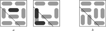
Figure 11: Application of the pocket algorithm to a dimer-configuration on the two-dimensional square lattice. In this problem, the maximum size of the pocket is $2$. The initial configuration $a$, the configuration after the first transformation, and the final configuration $b$ are shown.

6 Limitations and Extensions

As other powerful methods, the pivot cluster algorithm allows to solve basic computational problems for some systems, but fails abysmally for the vast majority. The main reason for failure is the presence of clusters which are too large, in applications where they leave only ‘uninteresting’ small clusters.

This phenomenon is familiar from spin-cluster algorithms, which, for example fail for frustrated or random spin models, thus providing strong motivation for many of the combinatorial techniques presented elsewhere in this book. Clearly, a single method cannot be highly optimized and completely general at the same time.

In the first place, the cluster pivot algorithm has not improved the notoriously difficult simulations for monodisperse hard disks at the liquid-solid transition density. This density is higher than the percolation threshold of the combined two-plate system comprising the original and the copy. Nevertheless, one might suppose that the presence of small clusters would generate fast non-local density fluctuations. Unfortunately, this has not been found to have much impact on the overall convergence times. A clear explanation of this finding is missing.

Another frustrating example is the Onsager problem of liquid crystals: hard cylindrical rods with diameter $D$, and length $L$, which undergo a isotropic-nematic transition at a volume fraction which goes to zero as the rods become more and more elongated [12].

$$\rho_{\text{iso}}\sim 3.3\frac{D}{L}\quad\text{for $D/L\rightarrow 0$}$$ (7)

This is analogous to what we found for binary mixtures, where the transition densities also go to zero with the ratio of the relevant length scales, and one might think that the cluster algorithm should work just as well as it does for binary mixtures.

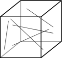
Figure 12: Hard rods of length $L$ and diameter $D$ in a test box of dimensions $L^{3}$. At the critical density for the isotropic-nematic transition, the volume fraction occupied by the rods goes to zero, but the cube is still opaque. This is due to the fact that the surface of a very thin object ($\sim LD$) is much larger than its volume ($\sim LD^{2}$).

Consider however a cube with edges of length $L$, filled with density $\rho_{\text{iso}}$ of rods (cf. Fig. 12). The question of the percolation threshold translates into asking what is the probability of another, identical, rod to hit one of the rods in the system.

$$\text{Volume of rods in cube of size}\ L^{3} \sim 3.3\ DL^{2}$$

Number of rods $$\sim\frac{13.2}{\pi}\ L/D$$

Surface $$\sim\frac{13.2}{\pi}\ L^{2}$$

During the performance of the cluster algorithm, an external rod will be moved into the test cube from elsewhere in the system. It is important that it does not generate a large number $n_{\text{rods}}$ of violations of the hard-core constraint with rods in the cube. We can orient the test cube such that the new rod comes in ‘straight’ and find that the number is given as

$$n_{\text{rods}}\sim\frac{\text{surface of rods in test cube}}{\text{surface of test cube}}\sim 4.2$$ (8)

This is what was indeed observed: the exterior rod will hit around $4$ other rods, this means that this system is far above the percolation threshold $n_{\text{rods}}=1$, and the cluster will contain essentially all the rods in the system.

The pivot cluster algorithm has been used in a series of studies of more realistic colloids, and has been extended to include a finite potential, in addition to the hard-sphere interaction [13].

Finally, the pivot cluster algorithm has been very successfully applied to the Ising model with fixed magnetization, where the number of “$+$” and of “$-$” spins are separately conserved. This is important in the context of lattice gases, which can be mapped onto the Ising model [14].

7 Acknowledgments

I would like to thank C. Dress, S. Bagnier, A. Buhot, L. Santen, and R. Moessner for stimulating collaborations over the last few years.

References

- [1] U. Wolff, Collective Monte Carlo Updating for Spin Systems, Phys. Rev. Lett. 62, 361 (1989)
- [2] H. G. Evertz, The Loop Algorithm, Adv. Phys. 52, 1 (2003)
- [3] C. Dress, W. Krauth, Cluster Algorithm for hard spheres and related systems, J. Phys. A: Math Gen. 28, L597 (1995)
- [4] W. Krauth, R. Moessner, Pocket Monte Carlo algorithm for classical doped dimer models, Phys. Rev. B 67, 064503 (2003)
- [5] W. Krauth, Statistical Mechanics: Algorithms and Computations, (Oxford University Press, 2004)
- [6] J. A. Cuesta, Fluid Mixtures of Parallel Hard Cubes, Phys. Rev. Lett. 76, 3742 (1996)
- [7] A. Buhot, W. Krauth, Numerical Solution of Hard-Core Mixtures, Phys. Rev. Lett. 80, 3787 (1998)
- [8] A. Buhot, W. Krauth, Phase Separation in Two-Dimensional Additive Mixtures, Phys. Rev. E 59, 2939 (1999)
- [9] L. Santen, W. Krauth, Absence of Thermodynamic Phase Transition in a Model Glass Former, Nature 405, 550 (2000)
- [10] L. Santen, W. Krauth, Liquid, Glass and Crystal in Two-dimensional Hard disks, cond-mat/0107459
- [11] D. A. Huse, W. Krauth, R. Moessner, S. L. Sondhi, Coulomb and Liquid Dimer Models in Three Dimensions, Phys. Rev. Lett. 91 167004 (2003)
- [12] P. G. de Gennes, The Physics of Liquid Crystals, (Oxford University Press, 1974)
- [13] J. G. Malherbe, S. Amokrane, Asymmetric mixture of hard particles with Yukawa attraction between unlike ones: a cluster algorithm simulation study, Mol. Phys. 97, 677 (1999)
- [14] J. R. Heringa and H. W. J. Blöte, The simple-cubic lattice gas with nearest-neighbour exclusion: Ising universality, Physica 232A, 369 (1996)