Temperature dependent Bogoliubov approximation in the classical fields approach to weakly interacting Bose gas

Abstract

A classical fields approximation to the finite temperature microcanonical thermodynamics of weakly interacting Bose gas is applied to the idealized case of atoms confined in a box with periodic boundary conditions. We analyze in some detail the microcanonical temperature in the model. We also analyze the spectral properties of classical amplitudes of the plane waves – the eigenmodes of the time averaged one–particle density matrix. Looking at the zero momentum component – the order parameter of the condensate, we obtain the nonperturbative results for the chemical potential. Analogous analysis of the other modes yields nonperturbative temperature dependent Bogoliubov frequencies and their damping rates. Damping rates are linear functions of momenta in the phonon range and show more complex behavior for the particle sector. Where available, we make comparison with the analytic estimates of these quantities.

I Introduction

Since the achievement of Bose-Einstein condensation in dilute atomic gases BEC there is a remarkable experimental activity in this area of physics. Quantum properties of the weakly interacting Bose gas are studied both close and away from thermal equilibrium. While in most cases the experiments are performed with as cold gas sample as possible, some experiments test the dependence of these properties on temperature. The central role in the theoretical studies of this system is played by the collective excitations. At and near zero temperature these collective excitations are described very well by the Bogoliubov approximation. Much less is known about the collective excitations at higher temperatures.

More generally, quantum theory of weakly interacting Bose gas at finite temperatures is still a challenge. To answer this challenge most researchers describe the system as consisting of two different, mutually interacting components: the condensate and the thermal cloud Stringari . This way a significant progress has been achieved in explaining such experimental observations as, for instance, temperature shifts and damping rates of various oscillation modes of the two component system Zaremba . The two component approaches, although successful, are unsatisfying in their underlying assumptions. The splitting of the gas at nonzero temperature into the condensate and the thermal cloud should be the result of the Bose statistics and of interactions.

In a series of papers several groups formulated the, so called, classical fields approximation classf ; OpEx ; Davis ; Oxford1 ; Oxford2 ; RapCom ; Castin . Within this formulation there are, however, two slightly different approaches. The group of ENS Castin developed the so called truncated Wigner method for Bose condensed gases. The main idea is to describe the total system by a classical field obeying the Gross–Pitaevskii equation. The classical field, except of a condensate component, contains also a stochastic part representing a thermal cloud. Mean values of observables are calculated as averages over an ensemble of classical fields which are chosen according to the Wigner quasi–distribution function of the initial thermal equilibrium density operator of the gas. This approach corresponds to the canonical description of the system where a temperature not energy is a control parameter.

The approach that we use has been formulated in OpEx ; Oxford1 and corresponds to the microcanonical description. This approximation, drawing from quantum optics, consists of replacing the quantum mechanical operators of highly occupied modes of the Bose field with complex c–number amplitudes. The idea of replacing the annihilation (creation) operators by c–number amplitudes is a straightforward generalization of Bogoliubov hypothesis to a case when large number of modes is macroscopically occupied. It is the aim of this paper to analyze the classical fields approximation in terms of such fundamental notions as the microcanonical temperature, the chemical potential and the quasiparticle excitations.

The paper is organized as follows: In Section II, for the sake of completeness, we briefly describe the classical fields approximation. In Section III we analyze the dynamical equations of the approximation from the point of view of underlying spectra. In Section IV the numerical results are discussed to support the analysis of Section III. In particular we show that the Bogoliubov energies at high temperature follow the gapless formula derived in Pethick . We also analyze the thermal damping rates of the modes. We find that they are proportional to momenta for the phonon excitations. The dependence of damping rates of particle–like modes on momentum is more complex showing the existence of bending points. We present some concluding remarks in Section V.

II Classical fields approximation

We consider $N$ identical atoms subject to Bose-Einstein statistics, confined to a cubic box of volume $V$ , with their atomic wave functions satisfying periodic boundary conditions. The atoms interact via contact potential characterized by the scattering length $a_{s}$. We use the method of second quantization. Our dynamical variable is a bosonic field operator $\hat{\Psi}({\bf r},t)$ that destroys a particle at position ${\bf r}$ and obeys standard bosonic commutation $[\hat{\Psi}({\bf r},t),\hat{\Psi}^{\dagger}({\bf r}^{\prime},t)]=\delta({\bf r}-{\bf r}^{\prime})$ relations. The Hamiltonian of the system reads:

$$H = \int d^{\,3}r\;\hat{\Psi}^{\dagger}({\bf r},t)\frac{p^{2}}{2m}\hat{\Psi}({\bf r},t)$$

$$+ \frac{2\pi\hbar^{2}a_{s}}{m}\int d^{\,3}r\;\hat{\Psi}^{\dagger}({\bf r},t)\hat{\Psi}^{\dagger}({\bf r},t)\hat{\Psi}({\bf r},t)\hat{\Psi}({\bf r},t)\;.$$

The Heisenberg equation of motion for the field operator follows:

$$i\hbar\frac{\partial\hat{\Psi}({\bf r},t)}{\partial t}= - \frac{\hbar^{2}}{2m}\nabla^{2}\,\hat{\Psi}({\bf r},t)$$ (2)

$$+ \frac{4\pi\hbar^{2}a_{s}}{m}\;\hat{\Psi}^{\dagger}({\bf r},t)\hat{\Psi}({\bf r},t)\hat{\Psi}({\bf r},t)\;.$$

We do not know how to solve this nonlinear operator equation. However, a natural simplification is possible for the degrees of freedom (modes) of the field, which are occupied by large number of atoms. Just like corresponding highly occupied modes of electromagnetic field, they can be described by c–number complex amplitudes rather than by their creation and annihilation operators. On the other hand the modes that are sparsely populated and require full quantum treatment, may be in the crudest approximation neglected.

The symmetry of the box with periodic boundary condition determines a natural set of modes for the thermal equilibrium states of atoms. The natural modes are simply the plane waves, with quantized momentum ${\bf p}=2\pi\hbar(n_{1},n_{2},n_{3})/L$ ($n_{i}$ being integer). Therefore, the field operator can be expanded in these modes:

$$\hat{\Psi}({\bf r},t)=\frac{1}{\sqrt{V}}\sum_{{\bf p}}\exp(-i{\bf p}{\bf r}/\hbar)\hat{a}_{{\bf p}}(t)\;.$$ (3)

Substituting the expansion (3) into (2) we get a set of nonlinear equations for the creation and annihilation operators of the plane wave modes:

$$\frac{d\hat{a}_{{\bf p}}(t)}{dt}=-i\frac{p^{2}}{2m\hbar}\hat{a}_{{\bf p}}-i\frac{g}{V\hbar}\sum_{{\bf q}_{1},{\bf q}_{2}}\hat{a}^{\dagger}_{{\bf q}_{1}}\hat{a}_{{\bf q}_{2}}\hat{a}_{{\bf p}+{\bf q}_{1}-{\bf q}_{2}}\;,$$ (4)

where the coupling $g$ is equal to:

$$g=\frac{4\pi\hbar^{2}a_{s}}{m}\;.$$ (5)

At this point we identify the set of highly occupied modes. By definition these are all long wave length degrees of freedom up to a maximal cut–off momentum ${\bf p}_{max}$. For these modes we replace the operators with complex amplitudes:

$$\hat{a}_{\bf p}=\sqrt{N}\alpha_{\bf p}$$ (6)

in such a way that the square of the modulus of the amplitude gives the fraction of atoms in a given mode. The above replacement is a direct generalization of the Bogoliubov hypothesis.

Confining our attention to the highly occupied modes we are reducing the dynamical equations to the set of nonlinear differential equations for the amplitudes:

$$\frac{d\alpha_{{\bf p}}(t)}{dt}=-i\frac{p^{2}}{2m\hbar}\alpha_{{\bf p}}-i\frac{gN}{V\hbar}\sum_{{\bf q}_{1},{\bf q}_{2}}\alpha^{*}_{{\bf q}_{1}}\alpha_{{\bf q}_{2}}\alpha_{{\bf p}+{\bf q}_{1}-{\bf q}_{2}}\;,$$ (7)

which may be solved numerically. Note that summation over momenta is truncated at $|{\bf q_{1}}|=|{\bf q_{2}}|=p_{max}$, where $p_{max}$ is a value of momentum of the highest mode which occupation is still macroscopic. In numerical implementation of the method the value of $p_{max}$ has to be determined self-consistently.

Eq. (7) is a momentum representation of the standard Gross–Pitaevskii equation. For numerical purposes it is convenient to switch to position representation which corresponds to the c–number version of the operator Eq. (2) on rectangular grid with the grid spacing defined by a cut–off momentum $\Delta x=\pi/p_{\max}$. In the classical fields method, a finite grid version of the Gross–Pitaevskii equation describes a total system – Bose-Einstein condensate and a thermal cloud.

This interpretation is shared by other groups which apply the classical fields method for microcanonical description of a cold Bose system Oxford1 ; Oxford2 ; Davis . In the recent paper Davis the value of the cut–off momentum has been chosen arbitrary. It means that only a fraction of all macroscopically occupied modes is taken into account, therefore in such a treatment there is no simple method of determination of a number of particles in the whole system. This leads to difficulties in assigning an absolute value of temperature and authors of Davis calculate some scaled temperature $T/N$ rather than $T$. We treat the problem of a cut–off momentum differently. In the present approach a number of classical modes, or equivalently a cut–off momentum, is an important physical parameter. We determine its value by requiring that an occupation of the cut–off momentum mode is equal to one. This is a kind of compromise as the validity of approximation is limited to modes with occupation large compared to one, but on the other hand we want to describe the whole system. Such a choice of the cut–off momentum ensures that the total occupation of modes with momenta not included in our computations is only a few percent even close to critical temperature. Moreover, we are able to determine the absolute (not scaled) value of temperature of the system.

The most important finding is OpEx ; Oxford1 that almost any initial condition of given number of atoms and given energy, after the transient thermalization period leads to a steady state that does not depend on the particular choice of initial conditions. This way we are able to produce a numerical version of fluctuating, weakly interacting Bose gas in the quantum degenerate region. Of course, at temperatures close to the critical one there are many highly occupied modes of the Bose field. All authors using the classical fields approximation identify the zero momentum component of the wave function with the condensate and all other components as a part of the thermal cloud. In a recent paper RapCom we have investigated this problem and came to the conclusion that the coarse graining due to the finite resolution of the realistic measurement, both in time and in space, reduces the pure state described by a single wave-function of the method to a mixed state in which there is no coherence between various momentum components of the field. Only with this interpretation the perfectly isolated system of a microcanonical approach may be viewed in quantum mechanics as a mixed state. In the next Sections we are going to spectrally analyze the long time solutions of Eqs. (7) to generalize the celebrated Bogoliubov approximation to higher temperatures.

III Excitation spectrum: approximate treatment

In this section we present an approximate analytical treatment of dynamical equations of the classical fields method. Under assumption of a steady–state evolution we discover some constants of motion what allows us to linearize the equations and find an excitation spectrum of the system. This approach leads to the notion of quasiparticles and the famous Bogoliubov–like spectrum.

The equations for complex amplitudes originating from the many body Hamiltonian are given by (7) and in a particular units of length (the size of the box $L$) and time ($mL^{2}/\hbar$) are:

$$\dot{\alpha}_{\bf p}=-i{{\bf p}^{2}\over 2}\alpha_{\bf p}-igN\sum_{{\bf l},{\bf m}}\alpha^{*}_{\bf l}\alpha_{\bf m}\alpha_{\bf p+l-m}\;.$$ (8)

The set of nonlinear Eqs. (8) has two constants of motion. The first is the total energy of the system, $E=N\sum_{{\bf k}}({\bf k}^{2}/2)n_{{\bf k}}+(gN/2)\sum_{\bf k,l,m}\alpha^{*}_{\bf k}\alpha^{*}_{\bf l}\alpha_{\bf m}\alpha_{\bf k+l-m}$ and the second is the number of particles $N\sum_{\bf k}n_{\bf k}$, where $n_{\bf k}=\alpha^{*}_{\bf k}\alpha_{\bf k}$. As we have already mentioned, the system reaches a thermal equilibrium OpEx after some transient time, which depends on constants of motion only. In this state, a condensate occupation undergoes small fluctuations around a well defined mean value. Neglecting these small fluctuations we assume that $n_{0}=\alpha^{*}_{0}\alpha_{0}$ is constant. A value of $n_{0}$ depends on the energy of the system and is close to one for small energies and decreases with increasing energy.

By rearranging terms in Eq. (8) we obtain the following equation for the amplitude of the condensate (${\bf p}=0$) mode:

$$\dot{\alpha}_{\bf 0}=-igN(2-n_{0})\alpha_{0}-igN\left(\sum_{{\bf k\neq 0}}\alpha_{\bf k}\alpha_{{\bf-k}}\right)\alpha_{0}^{*}+f_{\bf 0}(t)\;,$$ (9)

where

$$f_{\bf 0}(t)=-igN\sum_{\bf k\neq l;k,l\neq 0}\alpha^{*}_{\bf k}\alpha_{\bf l}\alpha_{\bf k-l}$$ (10)

plays a role of an external force. Eqs. (9) and its complex conjugate describe a pair of coupled harmonic oscillators driven by external forces. The coupling term, $\sum_{{\bf k\neq 0}}\alpha_{\bf k}\alpha_{{\bf-k}}$, is an anomalous density.

Figure 1: Fourier transform (in arbitrary units) of the anomalous density (peaks in the right part of the figure) and driving force (peaks in the left part of the figure) for various condensate occupations as indicated in the legend.

In general time dependence of both the anomalous density and driving force can be very complicated. However, in a steady state both these quantities simply oscillate in time:

$$\sum_{{\bf k\neq 0}}\alpha_{\bf k}\alpha_{{\bf-k}} = -\delta{\rm e}^{-2i(\phi+\mu t)}\;,$$ (11)

$$f_{\bf 0} = -\kappa\sqrt{n_{0}}{\rm e}^{-i(\phi+\mu t)}\;,$$ (12)

where $\mu$ plays a role of a chemical potential (as it can be seen later), $\phi$ is some constant phase while $\delta$ and $\kappa$ are (real) constants of motion depending on the energy and number of particles only. To support the assumed ansatz in Fig. 1 we show the Fourier transforms of the anomalous density and the driving force for three different values of the total energy. Indeed, independently of the energy, the Fourier transform of the anomalous density is sharply peaked at frequency which is larger by the factor of two than frequency corresponding to a peak in the spectrum of the driving force. Because of Eqs. (11) and (12) the equation for condensate amplitude has a simple solution:

$$\alpha_{\bf 0}=\sqrt{n_{0}}{\rm e}^{-i(\phi+\mu t)}\;,$$ (13)

what is consistent with our assumption that condensate population $n_{0}$ does not depend on time. Evidently, $\mu$ plays a role of a single particle energy in a condensate phase. The Eq. (9) gives also relation between chemical potential $\mu$ and other, introduced above parameters:

$$\mu=gN(2-n_{0})-gN(\delta+\kappa)\;.$$ (14)

The anomalous density $\delta$ is small at low energies or close to a critical energy, having maximum in between. The parameter $\kappa$ is very small at low energies but it grows continuously and gives a significant correction to the chemical potential at large energies. Our result can be compared to the one obtained from the two gas model $\mu=gN(2-n_{0})$ (see Fig. 2). Only at very small energies this model predicts a value of chemical potential correctly.

In Fig. 2 we show the chemical potential as a function of a condensate occupation (which is a monotonic function of temperature). We present two curves, both corresponding to the same value of the effective coupling $gN=731.5$, but for two different grid sizes. The number of grid points is equal to a number of macroscopically occupied modes. If we increase the number of macroscopically occupied modes while keeping population of the highest mode constant, we inevitably increase the total number of particles in the system, and simultaneously decrease the value of $g$ ($gN$ is fixed) Schmidt . Therefore, the curve corresponding to the larger grid (circles) describes larger system with weaker interactions as compared to the curve marked by boxes. In Fig. 3 we present the chemical potential as a function of the interaction strength $g$ at fixed condensate fraction $n_{0}=0.55$ and fixed effective coupling $gN=731.5$. According to the two gas model the chemical potential should be constant in such a case and its value, for chosen parameters, equals $\mu=1060$. This value is indicated in Fig. 3 by horizontal dashed line. Our results show that chemical potential depends on the interaction strength not only through the product $gN$. We expect that two gas model result can be reached in the limit of $g\rightarrow 0$, however calculation in this regime is a demanding task. In the inset we show the chemical potential versus condensate population (temperature) for fixed value of both: particle number $N$ and interaction strength $g$. The difference between the two gas model prediction and our result grows with temperature.

Figure 2: Chemical potential as a function of the condensate population for the effective coupling strength $gN=731.5$. Circles and boxes show numerical results obtained on the grids 36x36x36 and 16x16x16, respectively. The solid line comes from the formula derived within the two gas model.

Figure 3: Chemical potential as a function of the interaction strength $g$ alone for $gN=731.5$ and the condensate occupation $n_{0}=0.55$ (solid line is added to guide an eye). The horizontal dashed line indicates the value of the chemical potential obtained from the two gas model formula: $\mu=gN(2-n_{0})\approx 1060$. The inset shows, just like Fig. 2, the chemical potential as a function of the condensate population but for a constant number of atoms $N=235000$.

Now, we rearrange terms in the dynamical equation (8) for amplitudes of excited modes to get the following expression:

$$\dot{\alpha}_{\bf p}= - i\left({{\bf p}^{2}\over 2}+2gN\right)\alpha_{\bf p}$$ (15)

$$- igN\left(\alpha_{0}^{2}+\sum_{{\bf k}\neq 0}\alpha_{\bf k}\alpha_{{\bf-k}}\right)\alpha_{{\bf-p}}^{*}+f_{\bf p}\;,$$

where

$$f_{\bf p}=-igN\sum_{\bf k\neq-p,l;l\neq p}\alpha^{*}_{\bf k}\alpha_{\bf l}\alpha_{\bf p+k-l}$$ (16)

is a driving force of the $\alpha_{\bf p}$ mode. Guided by the previous experience, we expect that the driving force $f_{\bf p}$ becomes important at larger energies. However, its time dependence is not as simple as that of $f_{\bf 0}$. In the first approach we omit this force in our analytical treatment. We are well aware that doing this we loose very important contribution to the dynamics, nevertheless even this oversimplified analysis gives interesting physical insight.

After all the above simplification we get the set of coupled equations for amplitudes of $\alpha_{\bf p}$ and $\alpha^{*}_{\bf-p}$ modes. They describe excitation of the system by creation of correlated pair of particle with momentum p and a hole in the condensate with opposite momentum. The solution of this set reminds famous Bogoliubov transformation:

$$\alpha_{\bf p}={\rm e}^{-i\mu t}\left({\rm e}^{-i\epsilon_{p}t}\beta_{\bf p}+{\rm e}^{i\epsilon_{p}t}\frac{\epsilon_{p}-\omega_{p}}{gN(n_{0}-\delta)}\beta_{{\bf-p}}^{*}\right)\;,$$ (17)

where amplitudes $\beta_{\bf p}$ and $\beta_{\bf-p}^{*}$ are some constants, and $\epsilon_{p}$ is the temperature dependent Bogoliubov spectrum:

$$\epsilon_{p}=\sqrt{\omega_{p}^{2}-[gN(n_{0}-\delta)]^{2}}$$ (18)

and $\omega_{p}$ is:

$$\omega_{p}={p^{2}\over 2}+gN(n_{0}+\kappa+\delta)\;.$$ (19)

The amplitude of the $\alpha_{\bf p}$ mode is a superposition of two components: the one oscillating with frequency $\mu+\epsilon_{p}$ and the second with frequency $\mu-\epsilon_{p}$. Excitations are Bogoliubov quasiparticles. We see, that this well known fact is reproduced by the classical fields method and is also valid at higher temperatures and for large interaction strength (in fact it is valid up to a critical temperature what we will show in the next section). At low momenta both frequency components of the amplitude $\alpha_{\bf p}$ are comparable while at high momenta the amplitude of the negative frequency component vanishes. Eq. (18) predicts a gap, i.e., the energy of excitation does not tend to zero as the momentum ${\bf p}$ tends to zero. This result violates the Hugenholtz-Pines gapless theorem which shows that excitation spectrum is gapless. The reason is that in our analysis we have neglected the term $f_{\bf p}$. Inclusion of this term gives the correct gapless spectrum and allows for determination of Landau damping rates of excitations.

IV Numerical results

In this section we show results obtained from numerical solution of the dynamical Eqs. (8) and compare them with approximate analytical solutions. We focus on the thermodynamics of a uniform weakly interacting Bose gas in the equilibrium. Knowing the spectrum of the elementary excitations (quasiparticles) as well as their populations we deliver the scheme which assigns the temperature to the system. After that most of the thermodynamic properties of the system can be derived, for example, the condensate occupation as a function of temperature. On the other hand, the width of the quasiparticles originating from the finite lifetime of the elementary excitations allows one to investigate dissipative processes in the system.

As we have already mentioned in Section II instead of solving Eqs. (8) it is more convenient to transform them to the position representation what leads to the finite–grid version of the time–dependent Gross–Pitaevskii equation for a system of particles in a box with periodic boundary conditions. The equation is written as:

$$i\frac{\partial\Psi}{\partial t}=-\frac{1}{2}\nabla^{2}\Psi+gN|\Psi|^{2}\Psi\;,$$ (20)

where particular units for the length (which is the box size $L$) and the time $(mL^{2}/\hbar)$ are assumed and the coupling constant $g$ equals $4\pi a_{s}/L$ ($a_{s}$ being the scattering length). This equation has to be solved on a rectangular grid and the grid spacing $\Delta x$ determines the value of the cut–off momentum $p_{max}=\pi/\Delta x$. The initial wave function is generated from the ground state solution by its random disturbance followed by the normalization. The strength of the disturbance determines the total energy per particle. Both the energy and the particle number are preserved during the evolution of the Gross–Pitaevskii equation and the system reaches the same stationary state independently of the choice of the initial wave function provided that the energy and the particle number are kept constant.

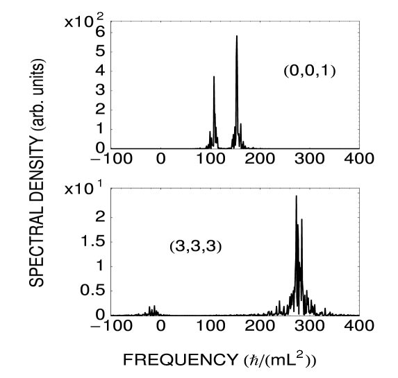
Figure 4: Fourier transform (in arbitrary units) of the (0,0,1) and (3,3,3) modes for gN=731.5 and $n_{0}=0.79$ (low temperature). Note the existence of two groups of frequencies.

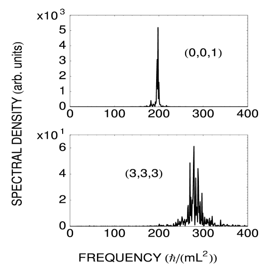
Figure 5: Fourier transform (in arbitrary units) of the (0,0,1) and (3,3,3) modes for gN=731.5 and $n_{0}=0.07$ (high temperature).

As it was discussed in the previous sections, the high energy solution of the Gross–Pitaevskii equation represents a pure state of the system and only time averaging procedure related to the nature of the observation process allows one to split the system to condensed and non–condensed parts. To this end, the time averaged (after the system enters the stationary state) single–particle density matrix is diagonalized and coherent modes (among them the condensate mode) and their populations are obtained. For a uniform gas the eigenfunctions of the single–particle density matrix are just the plane waves and the condensate is identified as the mode with zero momentum. Therefore, we propagate the high energy solution of the Gross–Pitaevskii equation and, at each time step, do the decomposition into plane waves by using the Fourier transform technique in spatial domain. In such a way we gain the time dependence of natural modes. Their spectrum (Fourier transform with respect to time) is plotted in Figs. 4 and 5 in the case of low and high temperatures, respectively, for modes $(0,0,1)$ and $(3,3,3)$. Typically, two groups of frequencies are visible in the spectrum and the separation between them increases with the mode energy. Moreover, increasing the energy of the mode leads also to the suppression of the lower frequencies group. Another important property is that the width of each group is getting broader when the temperature of the system is increasing.

The mean frequency of each group of frequencies is well described by the gapless Bogoliubov–like formula:

$$\epsilon_{p}=\sqrt{\left(\frac{p^{2}}{2}+gNn_{0}\right)^{2}-\left(gNn_{0}\right)^{2}}\;\;,$$ (21)

where $n_{0}$ is the condensate fraction. This simple generalization of the Bogoliubov formula is known as the Popov approximation Pethick . In Fig. 6, which is the case of $(1,1,1)$ mode, frequencies $\mu\pm\epsilon_{p}$ are marked by the vertical dotted lines whereas those given by the simplified expression (18) (when the driving force term is neglected) derived in the previous section by the dashed ones. Obviously, the formula (21) works better. The excellent agreement between the Bogoliubov–like expression (21) and numerical spectrum manifests itself in Fig. 7, where we plot the quasiparticle energies for various temperatures (condensate populations) and interaction strengths. Numerical points (marked by boxes, circles, and triangles) are calculated as the mean frequency values (with respect to $\mu$) corresponding to higher frequency groups, whereas the solid lines come from (21).

Figure 6: Fourier transform (in arbitrary units) of the (1,1,1) mode for gN=731.5 and $n_{0}=0.79$. Dotted vertical lines show frequencies obtained based on the formula (21) whereas dashed ones mark frequencies calculated from the simplified expression (18).

Figure 7: Dispersion relation for various interaction strengths and temperatures. Numerical results are marked by boxes ($gN=731.5$, $n_{0}=0.95$), circles ($gN=73.15$, $n_{0}=0.13$), and triangles ($gN=73.15$, $n_{0}=0.93$). Solid lines are obtained from the expression (21). Inset shows excellent agreement between the numerical data and formula (21) for all modes in the case of high temperature.

Figure 8: Quasiparticle energies as a function of inverse of the population for the system of $N=235000$ ($gN=731.5$) atoms for various temperatures. The upper set of data (circles) was obtained on the grid 36x36x36 and corresponds to the temperature of $9.37$ nK ($n_{0}=0.07$), the middle one (triangles) is the case of $4.27$ nK ($n_{0}=0.79$) and 24x24x24 grid whereas the lower set (marked by boxes) results from the 16x16x16 grid and gives the temperature of $1.80$ nK ($n_{0}=0.95$).

Approximate analytical solutions show that amplitudes $\alpha_{\bf p}$ and $\alpha^{*}_{\bf-p}$ oscillate with two frequencies. By taking appropriate linear combination of these amplitudes one can find normal modes of the system, i.e., modes oscillating with only one frequency. This transformation is just the transformation to Bogoliubov quasiparticle amplitudes. They can be regarded as an elementary excitations of the system. However, numerical results show that instead of two frequencies one obtains two distinct groups of sharp frequencies. For each positive frequency component $\mu+\epsilon$ (where $\epsilon$ corresponds to the frequency within the peak) there exists companion at the frequency $\mu-\epsilon$. Moreover, the phase difference of these components is equal to the corresponding one for mode ${\bf-p}$. The center of the higher frequencies group defines the energy of quasiparticle while the width of this group is related to its lifetime. By integrating over the quasiparticle spectrum one can get the occupation of the quasiparticle mode. In the phonon range the occupation of the quasiparticle must be obtained with the help of the Bogoliubov transformation. This task is simplified because of the phase relation mentioned above. Having energies of elementary excitations and their populations we can assign the temperature to the system Oxford2 . Since the modes are macroscopically occupied we expect that the equipartition relation is fulfilled, i.e., $Nn_{\bf p}(\epsilon_{\bf p}-\mu)=k_{B}T$ for each mode. As it is the case shows Fig. 8 where we plotted the energy of quasiparticles as a function of inverted population. Due to the equipartition relation this dependence should be linear and the slope of the line is just the temperature of the system. However, since the range of the ’y’ axis in Fig. 8 is rather large some details for small momenta might be hidden. Indeed, the presentation of the same results in a different form (see Fig. 9) shows departure of low energy modes (phonons) from the equipartition law. Finally, in Fig. 10 we plot the condensate occupation for various temperatures for the system built of $N=235000$ atoms. The dashed line in Fig. 10 shows the population of an ideal condensate of the same density. Although we can not precisely determine the value of critical temperature of finite size interacting gas, Fig. 10 clearly shows that the shift of the critical temperature is positive.

Figure 9: Verifying the equipartition relation we plot the expression $Nn_{\bf p}(\epsilon_{\bf p}-\mu)$ (in units of $\hbar^{2}/(mL^{2})$) for all modes. Note the imperfect equipartition for small momenta (phonon modes). Parameters are the same as in the case of middle set of data in Fig. 8.

Figure 10: Condensate occupation as a function of temperature for a uniform weakly interacting Bose gas; the scattering length equals $a_{s}=25$ nm ($gN=731.5$, $N=235000$). The dashed line shows the fraction of atoms in the condensate for the ideal gas of the same density (the critical temperature is about $T_{0}=7.1$ nK. The solid line is the fit: $1-(T/9.85)^{1.80}$.

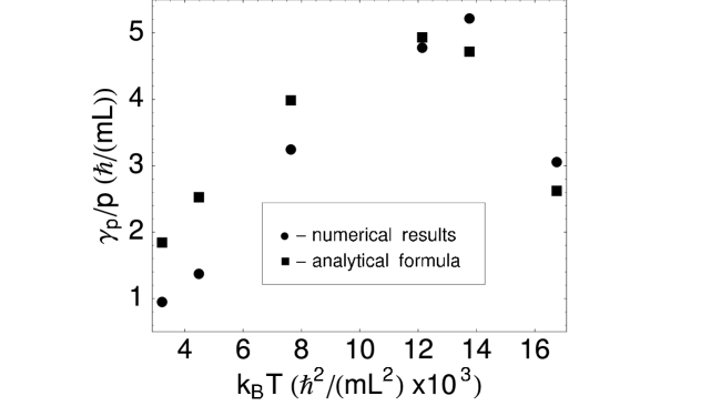
Figure 11: Comparison of the ratio $\gamma_{p}/p$ calculated numerically (circles) with that coming from the analytical formula (22) (and given by boxes) for various temperatures and $gN=731.5$.

Figure 12: The decay rates as a function of momentum for $gN=731.5$ and higher temperature ($n_{0}=0.48$). Both phonon–like and particle–like parts of spectrum are considered. Solid line follows the analytical formula (22).

Finally, we would like to discuss the damping of the quasiparticle modes. There exists analytical result for the decay rates of elementary excitations in a uniform Bose gas. At high temperatures ($k_{B}T\gg gN/V$) Landau processes dominate and the decay rate for the phonon–like part of the spectrum follows the formula Landau :

$$\gamma_{p}=\frac{3\pi^{3/2}}{2}\frac{k_{B}T}{gN/V}\left(\frac{N}{V}\,a^{3}_{s}\right)^{1/2}\frac{\epsilon_{p}}{\hbar}\;.$$ (22)

Since phonon energies depend linearly on the momentum, so do the decay rates. The ratio $\gamma_{p}/p$ is a function of temperature given by $\sim\!\!\sqrt{n_{0}}\,T$, where $n_{0}$ is the condensate fraction. In Fig. (11) we compare numerical results with the analytical expression (22). In order to determine the damping rates we average the spectrum of phonon–like modes over the angles in the momentum space and fit to the Lorentzian curve. The FWHM of the Lorentzian fit is just the damping rate. We see that both approaches agree quite well except of two first points. These points correspond to very low temperatures (approximately $2000$ and $4000$ in units of $\hbar^{2}/(mL^{2})$) and certainly the condition of the validity of analytical formula (22) is not fulfilled in this case since $gN/V$ is as high as $731.5$. However, in our method we can go beyond the phonon–like excitations and find the decay rates for particle–like part of the spectrum. In Fig. 12 we plot the damping rates for all momenta in the case of higher temperature. The solid line follows the analytical expression (22). The numerical results and formula (22) agree only for small momenta as it should be expected (see Fig. 11). The damping rates of particle–like excitations show the nonlinear dependence on the momentum.

V Conclusions

We have applied the classical fields approach to the weakly interacting Bose gas in a box with periodic boundary conditions. By Fourier transform we analyze the frequency dependence of amplitudes of eigenmodes of the system. We observe that the zero–momentum component of the field oscillates with single frequency which is identified as a chemical potential. We have obtained nonperturbative results for the chemical potential. For the physically relevant parameters it differs strongly from the simple two–gas formula. All other modes have much more complicated time evolution. Their spectra consist of two groups of frequencies displaced symmetrically with respect to the chemical potential. The center of gravity of each groups of frequencies agrees perfectly with a simple formula known as the Popov formula Pethick . The low momenta excitations have a phonon–like dispersion while for high momenta components the dispersion is of particle kind. Knowing the excitation spectrum of quasiparticles we are able to find also their populations and we can test the equipartition of the energy between the modes and then determine the temperature. The width of the spectrum is identified as the damping rate of quasiparticles. We observe that our nonperturbative results agree reasonably well with the analytic estimates for the phonon damping rates for high temperatures.

- (1) M.H. Anderson, J.R. Ensher, M.R. Matthews, C.E. Wieman, and E.A. Cornell, Science 269, 198 (1995); K.B. Davis, M.-O. Mewes, M.R. Andrews, N.J. van Druten, D.S. Durfee, D.M. Kurn, and W. Ketterle, Phys. Rev. Lett. 75, 3969 (1995); C.C. Bradley, C.A. Sackett, J.J. Tollett, and R.G. Hulet, Phys. Rev. Lett. 75, 1687 (1995) and Erratum 79, 1170(E) (1997).
- (2) F. Dalfovo, S. Giorgini, L.P. Pitaevskii, and S. Stringari, Rev. Mod. Phys. 71, 463 (1999).
- (3) E. Zaremba, A. Griffin, and T. Nikuni, Phys. Rev. A 57, 4695 (1998); B. Jackson and E. Zaremba, Phys. Rev. Lett. 88, 180402 (2002); B. Jackson and E. Zaremba, Phys. Rev. A 66, 033606 (2002); B. Jackson and E. Zaremba, New J. Phys. 5, 88 (2003).
- (4) B.V. Svistunov, J. Moscow Phys. Soc. 1, 373 (1991); K. Damle, S.N. Majumdar, and S. Sachdev, Phys. Rev. A 54, 5037 (1996); Yu. Kagan and B.V. Svistunov, Phys. Rev. Lett. 79, 3331 (1997); N.G. Berloff and B.V. Svistunov, Phys. Rev. A 66, 013603 (2002).
- (5) K. Góral, M. Gajda, and K. Rza̧żewski, Opt. Express 8, 92 (2001).
- (6) M.J. Davis, S.A. Morgan, and K. Burnett, Phys. Rev. Lett. 87, 160402 (2001); M.J. Davis, R.J. Ballagh, and K. Burnett, J. Phys. B 34, 4487 (2001).
- (7) M.J. Davis, S.A. Morgan, and K. Burnett, Phys. Rev. A 66, 053618 (2002).
- (8) M.J. Davis and S.A. Morgan, cond-mat/0307155.
- (9) K. Góral, M. Gajda, and K. Rza̧żewski, Phys. Rev. A 66, 051602 (2002).
- (10) I. Carusotto and Y. Castin, J. Phys. B 34, 4589 (2001); A. Sinatra, C. Lobo, and Y. Castin, J. Phys. B 35, 3599 (2002); I. Carusotto and Y. Castin, Phys. Rev. Lett. 90, 030401 (2003).
- (11) see for instance C. J. Pethick and H. Smith, Bose–Eintein Condensation in Dilute Gases (Cambridge University Press, New York, 2002), p. 225.
- (12) H. Schmidt, K. Góral, F. Floegel, M. Gajda, and K. Rza̧żewski, J. Opt. B 5, S96 (2003).
- (13) N.M. Hugenholtz and D. Pines, Phys. Rev. 116, 489 (1959).
- (14) P.O. Fedichev, G.V. Shlyapnikov, and J.T.M. Walraven, Phys. Rev. Lett. 80, 2269 (1998); P.O. Fedichev and G.V. Shlyapnikov, Phys. Rev. A 58, 3146 (1998).