Intrinsic Friction of Monolayers Adsorbed on Solid Surfaces.

O.Bénichou¹, A.M.Cazabat¹, J.De Coninck², M.Moreau³ and G.Oshanin^3,4
1 Laboratoire de Physique de la Matière Condensée,
Collège de France, 11 Place M.Berthelot, 75252 Paris Cedex 05, France
² Centre de Recherche en Modélisation Moléculaire,
Université de Mons-Hainaut, 20 Place du Parc, 7000 Mons, Belgium
³ Laboratoire de Physique Théorique des Liquides,
Université Paris 6, 4 Place Jussieu, 75252 Paris, France
⁴ Max-Planck-Institut für Metallforshung
Heisenbergstr. 3, 70569 Stuttgart, Germany

ABSTRACT

We overview recent results on intrinsic frictional properties of adsorbed monolayers, composed of mobile hard-core particles undergoing continuous exchanges with a vapor phase. In terms of a dynamical master equation approach we determine the velocity of a biased impure molecule - the tracer particle (TP), constrained to move inside the adsorbed monolayer probing its frictional properties, define the frictional forces exerted by the monolayer on the TP, as well as the particles density distribution in the monolayer.

INTRODUCTION

Monolayers emerging on solid surfaces exposed to a vapor phase are important in different backgrounds, including such technological and material processing operations as, e.g., coating, gluing or lubrication. Knowledge of their intrinsic frictional properties is important for understanding of different transport processes taking place within molecular films, film’s stability, as well as spreading of ultrathin liquid films on solid surfaces [1], spontaneous or forced dewetting of monolayers [2, 3] or island formation [4].

Since the early works of Langmuir, much effort has been invested in the analysis of the equilibrium properties of the adsorbed films [5]. Significant analytical results have been obtained predicting different phase transitions and ordering phenomena. As well, some approximate results have been obtained for both dynamics of isolated non-interacting adatoms on corrugated surfaces and collective diffusion, describing spreading of the macroscopic density fluctuations in interacting adsorbates [6].

Another important aspect of dynamical behavior concerns tracer diffusion in adsorbates, which is observed experimentally in STM or field ion measurements and provides a useful information about adsorbate’s viscosity or intrinsic friction. This problem is not only a challenging question in its own right due to emerging non-trivial, essentially cooperative behavior, but is also crucial for understanding of various dynamical processes taking place on solid surfaces. Most of available theoretical studies of tracer diffusion in adsorbed layers (see, e.g., [7]) exclude, however, the possibility of particles exchanges with the vapor, which limits their application to the analysis of behavior in realistic systems.

Here we focus on this important problem and provide a theoretical description of the properties of tracer diffusion in adsorbed monolayers in contact with a vapor phase. More specifically, the system we consider consists of (a) a solid substrate, which is modelled in a usual fashion as a regular lattice of adsorption sites; (b) a monolayer of adsorbed, mobile hard-core particles in contact with a vapor and (c) a single hard-core tracer particle (TP). We suppose that the monolayer particles move randomly along the lattice by performing symmetric hopping motion between the neighboring lattice sites, which process is constrained by mutual hard-core interactions, and may desorb from and adsorb onto the lattice from the vapor with some prescribed rates dependent on the vapor pressure, temperature and the interactions with the solid substrate. In contrast, the tracer particle is constrained to move along the lattice only, (i.e. it can not desorb to the vapor), and is subject to a constant external force of an arbitrary magnitude $E$. Hence, the TP performs a biased random walk, constrained by the hard-core interactions with the monolayer particles, and always remains within the monolayer, probing its frictional properties.

The questions we address here are the following: First, we aim to determine the force-velocity relation, i.e., the dependence of the TP terminal velocity $V_{tr}(E)$ on the magnitude of the applied external force. Next, we study the form of the force-velocity relation in the limit of a vanishingly small external bias. This allows us, in particular, to show that the frictional force exerted on the TP by the monolayer particles is viscous, and to evaluate the corresponding friction coefficient. Lastly, we analyze how the biased TP perturbs the particles density distribution in the monolayer; we proceed to show that there are stationary density profiles around the TP, which mirror a remarkable cooperative behavior. We also consider the case of monolayers sandwiched between two solid surfaces and demonstrate that here the cooperative phenomena are dramatically enhanced. Detailed account of these results can be found in the original papers [10, 11, 12, 13].

We finally remark that our analysis can be viewed from a different perspective. On the one hand, the system under study represents a certain generalization of the ”tracer diffusion in a hard-core lattice gas” problem (see, e.g., [7]) to the case where the random walk performed by the TP is biased and the number of particles in the monolayer is not explicitly conserved, due to exchanges with the reservoir. We recall that even this, by now classic model constitutes a many-body problem for which no exact general expression of the tracer diffusion coefficient $D_{tr}$ is known. On the other hand, our model provides a novel example of the so called “dynamical percolation” models (see, e.g. Ref.[8] for a review), in which the monolayer particles act as a fluctuating environment, which hinders the motion of an impure molecule, say, a charge carrier. Lastly, we note that the model under study can be thought of as some simplified picture of the stagnant layers emerging in liquids being in contact with a solid body. It is well known (see, e.g. Ref.[9]) that liquids in close vicinity of a solid interfaces - at distances within a few molecular diameters, do possess completely different physical properties compared to those characterizing the bulk phase. In this ”stagnant” region, in which an intrinsically disordered liquid phase is spanned by and contends with the ordering potential of the solid, liquid’s viscosity is drastically enhanced and transport processes are essentially hindered. Thus our model can be viewed as a two-level approximate model of this challenging physical system, in which the reservoir mimics the bulk fluid phase with very rapid transport, while the adsorbed monolayer represents the stagnant layer emerging on the solid-liquid interface.

THE MODEL AND THE EVOLUTION EQUATIONS

Consider a two-dimensional solid surface with some concentration of adsorption sites, which is brought in contact with a reservoir containing identic, electrically neutral particles - a vapor phase (Fig.5), maintained at a constant pressure. For simplicity of exposition, we assume here that adsorption sites form a regular square lattice of spacing $\sigma$. We suppose next that the reservoir particles may adsorb onto any vacant adsorption site at a fixed rate $f/\tau^{*}$, which rate depends on the vapor pressure and the energy gain due to the adsorption event. Further on, the adsorbed particles may move randomly along the lattice by hopping at a rate $1/4\tau^{*}$ to any of $4$ neighboring adsorption sites, which process is constrained by hard-core exclusion preventing multiple occupancy of any of the sites. Lastly, the adsorbed particles may desorb from the lattice back to the reservoir at rate $g/\tau^{*}$, which is dependent on the barrier against desorption. Both $f$ and $g$ are site and environment independent.

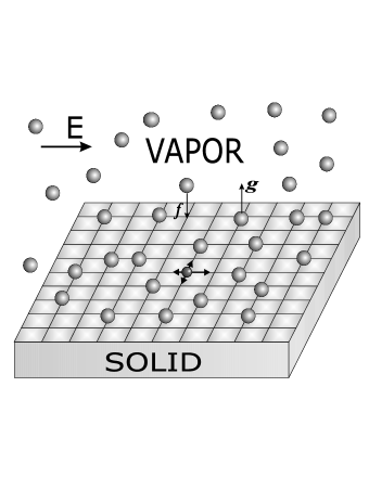
Figure 1: Adsorbed monolayer in contact with a vapor. Grey spheres denote the monolayer (vapor) particles; the smaller black sphere stands for the driven TP.

Further on, at $t=0$ we introduce at the lattice origin an extra hard-core particle, whose motion we would like to follow; position of this particle at time $t$ is denoted as ${\bf R}_{tr}$. We stipulate that the TP can not desorb from the lattice and that it is subject to some external driving force, which favors its jumps into a preferential direction. Physically, this situation may be realized if the TP is charged, while the monolayer particles are neutral, and the whole system is subject to external electric field. The TP transition probabilities are determined by:

$$p_{\nu}=\frac{\exp\Big{[}\frac{\beta}{2}({\bf E\cdot e}_{\boldsymbol{\nu}})\Big{]}}{\sum_{\mu}\exp\Big{[}\frac{\beta}{2}({\bf E\cdot e}_{\boldsymbol{\mu}})\Big{]}},$$ (1)

where $\beta$ is the reciprocal temperature, $({\bf E\cdot e})$ stands for the scalar product, the charge of the TP is set equal to unity and the sum with the subscript $\mu$ denotes summation over all possible orientations of the vector ${\boldsymbol{e}_{\mu}}$; that is, $\mu=\{\pm 1,\pm 2\}$. We suppose here that the external force ${\bf E}$ is oriented according to the unit vector ${\bf e_{1}}$.

In the general $d$-dimensional case, the time evolution of $P({\bf R_{tr}},\eta;t)$ - the joint probability of finding at time $t$ the TP at the site ${\bf R_{tr}}$ and all adsorbed particles in the configuration $\eta$, where $\eta\equiv\{\eta({\bf R})\}$ denotes the entire set of the occupation variables of different sites, obeys the following Master equation [10, 11, 12, 13]

$$\partial_{t}P({\bf R_{tr}},\eta;t)=\frac{1}{2d\tau^{*}}\sum_{\mu=1}^{d}\;\sum_{{\bf r}\neq{\bf R_{tr}}-{\bf e}_{\boldsymbol{\mu}},{\bf R_{tr}}}\;\Big{\{}P({\bf R_{tr}},\eta^{{\bf r},\mu};t)-P({\bf R_{tr}},\eta;t)\Big{\}}$$ (2)

$$+ \frac{1}{\tau}\sum_{\mu}p_{\mu}\Big{\{}\left(1-\eta({\bf R_{tr}})\right)P({\bf R_{tr}}-{\bf e}_{\boldsymbol{\mu}},\eta;t)-\left(1-\eta({\bf R_{tr}}+{\bf e}_{\boldsymbol{\mu}})\right)P({\bf R_{tr}},\eta;t)\Big{\}}$$

$$+ \frac{g}{\tau^{*}}\sum_{{\bf r}\neq{\bf R_{tr}}}\;\Big{\{}\left(1-\eta({\bf r})\right)P({\bf R_{tr}},\hat{\eta}^{{\bf r}};t)-\eta({\bf r})P({\bf R_{tr}},\eta;t)\Big{\}}$$

$$+ \frac{f}{\tau^{*}}\sum_{{\bf r}\neq{\bf R_{tr}}}\;\Big{\{}\eta({\bf r})P({\bf R_{tr}},\hat{\eta}^{{\bf r}};t)-\left(1-\eta({\bf r})\right)P({\bf R_{tr}},\eta;t)\Big{\}}.$$

where $\eta^{{\bf r},\nu}$ is the configuration obtained from $\eta$ by the Kawasaki-type exchange of the occupation variables of two neighboring sites ${\bf r}$ and ${\bf r+e}_{\boldsymbol{\nu}}$, and ${\hat{\eta}}^{\bf r}$ - a configuration obtained from the original $\eta$ by the replacement $\eta({\bf r})\to 1-\eta({\bf r})$, which corresponds to the Glauber-type flip of the occupation variable due to the adsorption/desorption events.

The mean velocity $V_{tr}(t)$ of the TP can be obtained by multiplying both sides of Eq.(2) by $({\bf R_{tr}\cdot e_{1}})$ and summing over all possible configurations $({\bf R_{tr}},\eta)$, which yields

$$V_{tr}(t)\equiv\frac{d}{dt}\;\sum_{{\bf R_{tr}},\eta}({\bf R_{tr}\cdot e_{1}})P({\bf R_{tr}},\eta;t)=\frac{\sigma}{\tau}\Big{\{}p_{1}\Big{(}1-k({\bf e_{1}};t)\Big{)}-p_{-1}\Big{(}1-k({\bf e_{-1}};t)\Big{)}\Big{\}},$$ (3)

where

$$k({\boldsymbol{\lambda}};t)\equiv\sum_{{\bf R_{tr}},\eta}\eta({\bf R_{tr}}+{\boldsymbol{\lambda}})P({\bf R_{tr}},\eta;t)$$ (4)

is the probability of having at time t an adsorbed particle at position ${\boldsymbol{\lambda}}$, defined in the frame of reference moving with the TP. In other words, $k({\boldsymbol{\lambda}};t)$ can be thought of as being the density profile in the adsorbed monolayer as seen from the moving TP.

Note that Eq.(3) signifies that the TP velocity is dependent on the monolayer particles density in its immediate vicinity. If the monolayer is perfectly stirred, i.e., if $k({\boldsymbol{\lambda}};t)=\rho_{s}$ everywhere, where $\rho_{s}=f/(g+f)$ is the Langmuir adsorption isotherm [5], one would obtain from Eq.(3) a trivial mean-field result $V_{tr}^{(0)}=(p_{1}-p_{-1})(1-\rho_{s})(\sigma/\tau)$, which states that the only effect of the medium on the TP dynamics is that its jump time $\tau$ is renormalized by $(1-\rho_{s})^{-1}$. We proceed to show, however, that $k({\boldsymbol{\lambda}};t)$ is different from $\rho_{s}$ everywhere, except for $|\boldsymbol{\lambda}|\to\infty$. This means that the TP strongly perturbs the monolayer.

The method of solution of Eq.(2) and (3) has been amply discussed in [10, 11, 12, 13]. Here we merely present the results.

RESULTS FOR ONE-DIMENSIONAL MONOLAYERS

We focus here on the one-dimensional lattice, which is appropriate to adsorption on polymer chains [14], and on the limit $t\to\infty$. In this case, the stationary particles density profile, as seen from steadily moving TP, has the following form:

$$k_{n}\equiv k(\lambda)=\rho_{s}+K_{\pm}exp\Big{(}-\sigma|n|/\lambda_{\pm}\Big{)},\;\;\;\lambda=\sigma n,\;\;\;n\in Z,$$ (5)

where the characteristic lengths $\lambda_{\pm}$ obey

$$\lambda_{\pm}=\;\mp\;\sigma\;ln^{-1}\Big{[}\frac{A_{1}+A_{-1}+2(f+g)\mp\sqrt{\Big{(}A_{1}+A_{-1}+2(f+g)\Big{)}^{2}-4A_{1}A_{-1}}}{2A_{1}}\Big{]},$$ (6)

the amplitudes $K_{\pm}$ are given by

$$K_{+}=\rho_{s}\frac{A_{1}-A_{-1}}{A_{-1}-A_{1}\exp(-\sigma/\lambda_{+})},\;\;\;K_{-}=\rho_{s}\frac{A_{1}-A_{-1}}{A_{-1}\exp(-\sigma/\lambda_{-})-A_{1}},$$ (7)

the terminal velocity $V_{tr}=\sigma(A_{1}-A_{-1})/2\tau^{*}$, while $A_{1}$ and $A_{-1}$ obey:

$$A_{1}=1+\frac{p_{1}\tau^{*}}{\tau}\Big{[}1-\rho_{s}-\rho_{s}\frac{A_{1}-A_{-1}}{A_{-1}exp(\sigma/\lambda_{+})-A_{1}}\Big{]},$$ (8)

and

$$A_{-1}=1+\frac{p_{-1}\tau^{*}}{\tau}\Big{[}1-\rho_{s}-\rho_{s}\frac{A_{1}-A_{-1}}{A_{-1}-A_{1}exp(\sigma/\lambda_{-})}\Big{]}.$$ (9)

Figure 2: The TP velocity as a function of the adsorption probability $f$ at different values of $g$. The TP hopping probabilities are $p_{1}=0.6$ and $p_{-1}=0.4$. The solid lines give the analytical solution while the squares denote the Monte-Carlo simulations results. Upper curves correspond to $g=0.8$, the intermediate - to $g=0.5$ and the lower - to $g=0.3$, respectively.

Note that $\lambda_{-}>\lambda_{+}$, and consequently, the local density past the TP approaches its non-perturbed value $\rho_{s}$ slower than in front of it. Next, $K_{+}$ is always positive, while $K_{-}<0$; this means that the density profile is a non-monotonous function of $\lambda$ and is characterized by a jammed region in front of the TP, in which the local density is higher than $\rho_{s}$, and a depleted region past the TP in which the density is lower than $\rho_{s}$.

For arbitrary values of $p$, $f$ and $g$ the parameters $A_{\pm 1}$, Eqs.(8) and (9), and consequently, $V_{tr}$ can be determined only numerically (see Figs.2 to 4). However, $V_{tr}$ can be found analytically in the limit $E\to 0$. In the leading in $E$ order, we find

$$V_{tr}\sim\zeta^{-1}E,$$ (10)

which relation is an analog of the Stokes formula for driven motion in a 1D adsorbed monolayer undergoing continuous particles exchanges with the vapor phase and signifies that the frictional force exerted on the TP by the monolayer particles is $viscous$. The friction coefficient $\zeta$ is given explicitly by

$$\zeta=\frac{2\tau}{\beta\sigma^{2}(1-\rho_{s})}\Big{[}1+\frac{\rho_{s}\tau^{*}}{\tau(f+g)}\frac{2}{1+\sqrt{1+2(1+\tau^{*}(1-\rho_{s})/\tau)/(f+g)}}\Big{]}$$ (11)

Note that the friction coefficient in Eq.(11) can be written down as the sum of two contributions $\zeta=\zeta_{cm}+\zeta_{coop}$. The first one, $\zeta_{cm}=2\tau/\beta\sigma^{2}(1-\rho_{s})$ is a typical mean-field result and corresponds to a perfectly homogeneous monolayer. The second one,

$$\zeta_{coop}=\frac{8\tau^{*}\rho_{s}}{\beta\sigma^{2}(1-\rho_{s})(f+g)}\frac{1}{1+\sqrt{1+2(1+\tau^{*}(1-\rho_{s})/\tau)/(f+g)}},$$ (12)

has a more complicated origin and reflects a cooperative behavior emerging in the monolayer, associated with the formation of inhomogeneous density profiles (see Fig.3) - the formation of a “traffic jam” in front of the TP and a “depleted” region past the TP (for more details, see [10]). The characteristic lengths of these two regions as well as the amplitudes $K_{\pm}$ depend on the magnitude of the TP velocity; on the other hand, the TP velocity is itself dependent on the density profiles, in virtue of Eq.(3). This results in an intricate interplay between the jamming effect of the TP and smoothening of the created inhomogeneities by diffusive processes. Note also that cooperative behavior becomes most prominent in the conserved particle number limit. Setting $f,g\to 0$, while keeping their ratio fixed (which insures that $\rho_{s}$ stays constant), one notices that $\zeta_{coop}$ gets infinitely large. As a matter of fact, in such a situation no stationary density profiles around the TP exist; the size of both the ”traffic jam” and depleted regions grow in proportion to the TP mean displacement $\overline{X_{tr}(t)}\sim\sqrt{t}$ [15].

Figure 3: Density profile around stationary moving TP for $f=0.1$, $g=0.3$ and $p=0.98$. The solid line is the plot of the analytical solution. Squares are the MC results.

Consider finally the situation with $E=0$, in which case the terminal velocity vanishes and one expects conventional diffusive motion such that

$$\overline{X_{tr}^{2}(t)}=2D_{tr}t,$$ (13)

where $D_{tr}$ is the diffusion coefficient. We can evaluate $D_{tr}$ if we assume that the Einstein relation $D_{tr}=\beta/\zeta$ holds, which yields

$$D_{tr}=\frac{\sigma^{2}(1-\rho_{s})}{2\tau}\left\{1+\frac{\rho_{s}\tau^{*}}{\tau(f+g)}\frac{2}{1+\sqrt{1+2(1+\tau^{*}(1-\rho_{s})/\tau)/(f+g)}}\right\}^{-1}.$$ (14)

Monte Carlo simulations evidently confirm our prediction for $D_{tr}$ (see Fig.4).

Figure 4: The TP self-diffusion coefficient vs the adsorption probability $f$. Notations and values of $g$ are the same as in Figs.2.

RESULTS FOR TWO-DIMENSIONAL ADSORBED MONOLAYERS

We turn now to the case of a 2D substrate. In this case, the general solution for the density profiles, in the frame of reference moving with the TP, reads [10, 11, 12, 13]:

$$k({\bf\lambda})=k_{n_{1},n_{2}}=\rho_{s}+\alpha^{-1}\Big{\{}\sum_{\nu}A_{\nu}h({\bf e}_{\bf\nu})\nabla_{-\nu}F_{n_{1},n_{2}}-\rho_{s}(A_{1}-A_{-1})(\nabla_{1}-\nabla_{-1})F_{n_{1},n_{2}}\Big{\}}$$ (15)

with

$$F_{n_{1},n_{2}}=\left(\frac{A_{-1}}{A_{1}}\right)^{n_{1}/2}\int_{0}^{\infty}e^{-t}{\rm I}_{n_{1}}\left(2\alpha^{-1}\sqrt{A_{1}A_{-1}}t\right){\rm I}_{n_{2}}\left(2\alpha^{-1}A_{2}t\right){\rm d}t,$$ (16)

where ${\rm I}_{n}(z)$ stands for the modified Bessel function, the coefficients $A_{\nu}$ are determined implicitly as the solution of the following system of three non-linear matrix equations

$$\forall\nu=\{\pm 1,2\},\;\;\;\;A_{\nu}=1+\frac{4\tau^{*}}{\tau}p_{\nu}\left\{1-\rho_{s}-\rho_{s}(A_{1}-A_{-1})\frac{\det\tilde{C}_{\nu}}{\det\tilde{C}}\right\},$$ (17)

$$\tilde{C}=\begin{pmatrix}A_{1}\nabla_{-1}F_{\bf e_{1}}-\alpha&A_{-1}\nabla_{1}F_{\bf e_{1}}&A_{2}\nabla_{-2}F_{\bf e_{1}}\\ A_{1}\nabla_{-1}F_{\bf e_{-1}}&A_{-1}\nabla_{1}F_{\bf e_{-1}}-\alpha&A_{2}\nabla_{-2}F_{\bf e_{-1}}\\ A_{1}\nabla_{-1}F_{\bf e_{2}}&A_{-1}\nabla_{1}F_{\bf e_{2}}&A_{2}\nabla_{-2}F_{\bf e_{2}}-\alpha\end{pmatrix}.$$ (18)

the matrix $\tilde{C_{\nu}}$ stands for the matrix obtained from $\tilde{C}$ by replacing the $\nu$-th column by the column-vector $\tilde{F}$,

$$\tilde{F}=\begin{pmatrix}(\nabla_{1}-\nabla_{-1})F_{\bf e_{1}}\\ (\nabla_{1}-\nabla_{-1})F_{\bf e_{-1}}\\ (\nabla_{1}-\nabla_{-1})F_{\bf e_{2}}\end{pmatrix},$$ (19)

while $h({\bf e}_{\bf\nu})$ are expressed in terms of $A_{\nu}$ as

$$h({\bf e}_{\bf\nu})=(1-\rho_{s})+\frac{\tau}{4\tau^{*}p_{\nu}}(1-A_{\nu}).$$ (20)

Lastly, we find that the TP velocity obeys

$$V_{tr}=\frac{\sigma}{\tau}(p_{1}-p_{-1})(1-\rho_{s})\Big{\{}1+\rho_{s}\frac{4\tau^{*}}{\tau}\frac{p_{1}\det\tilde{C}_{1}-p_{-1}\det\tilde{C}_{-1}}{\det\tilde{C}}\Big{\}}^{-1}.$$ (21)

Non-linear Eqs.(15) are quite complex and their explicit solution can not be obtained analytically. Typical density profiles are depicted in Fig.5 and are characterized by a condensed, traffic-jam-like region in front of the stationary moving TP, and a depleted by particles region past the TP.

The asymptotical behavior of the density profiles at large distances from the TP is quite spectacular. In front of the TP, the deviation $h_{n,0}=k_{n,0}-\rho_{s}$ always decays exponentially with the distance:

$$h_{n,0}\sim K_{+}\frac{\exp\Big{(}-n/\lambda_{+}\Big{)}}{n^{1/2}},\;\;\;\lambda_{+}=\ln^{-1}\Big{(}\frac{1}{A_{-1}}\left\{\frac{\alpha}{2}-A_{2}+\sqrt{\left(\frac{\alpha}{2}-A_{2}\right)^{2}-A_{1}A_{-1}}\right\}\Big{)}.$$ (22)

On contrary, the behavior past the TP depends qualitatively on the physical situation. In the general case when exchanges with the vapor phase are allowed, the decay of the density profiles is still exponential:

$$h_{-n,0}\sim K_{-}\frac{\exp\Big{(}-n/\lambda_{-}\Big{)}}{n^{1/2}},\;\;\;\lambda_{-}=-\ln^{-1}\Big{(}\frac{1}{A_{-1}}\left\{\frac{\alpha}{2}-A_{2}-\sqrt{\left(\frac{\alpha}{2}-A_{2}\right)^{2}-A_{1}A_{-1}}\right\}\Big{)}$$ (23)

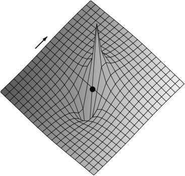
Figure 5: Typical density profiles in 2D case. The arrow shows the direction of external field.

In the conserved particles number limit, which can be realized for the monolayers sandwiched in a narrow gap between two solid surfaces, $\lambda_{-}$ becomes infinitely large and the deviation of the particle density from the equilibrium value $\rho_{s}$ follows

$$h_{-n,0}=-\frac{K_{-}^{\prime}}{n^{3/2}}\left(1+\frac{3}{8n}+{\mathcal{O}}\Big{(}\frac{1}{n^{2}}\Big{)}\right).$$ (24)

Remarkably enough, in this case the correlations between the TP position and the particles distribution vanish algebraically slow with the distance! This implies that mixing of the monolayer is not efficient enough to prevent the appearance of the quasi-long-range order and the medium ”remembers” the passage of the TP on a long time and space scale.

Now, in the limit $\beta E\ll 1$ we find a Stokes-type formula of the form $V_{tr}\sim E/\zeta$, where

$$\zeta=\frac{4\tau}{\beta\sigma^{2}(1-\rho_{s})}\left\{1+\frac{\tau^{*}}{\tau}\frac{\rho_{s}}{\Big{(}f+g+1+\tau^{*}(1-\rho_{s})/\tau\Big{)}\Big{(}{\cal L}(x)-x\Big{)}}\right\},$$ (25)

with

$$x=\frac{1}{2}\frac{1+\tau^{*}(1-\rho_{s})/\tau}{f+g+1+\tau^{*}(1-\rho_{s})/\tau}\;\;\;\text{and}\;\;\;{\cal L}(x)\equiv\left\{\int_{0}^{\infty}e^{-t}\Big{(}({\rm I}_{0}(xt)-{\rm I}_{2}(xt)){\rm I}_{0}(xt){\rm d}t\right\}^{-1}.$$ (26)

Note that we again are able to single out two physically meaningful contributions to the friction coefficient $\zeta$. Namely, the first term on the rhs of Eq.(25) is just the mean-field-type result corresponding to a perfectly stirred monolayer, in which correlations between the TP and the monolayer particles are discarded. The second term, similarly to the 1D case, mirrors the cooperative behavior emerging in the monolayer and is associated with the backflow effects. In contrast to the 1D case, however, the contribution stemming out of the cooperative effects remains finite in the conserved particles limit.

Lastly, we estimate the TP diffusion coefficient $D_{tr}=\beta^{-1}\zeta^{-1}$ as

$$D_{tr}=\frac{\sigma^{2}}{4\tau}(1-\rho_{s})\left\{1-\frac{2\rho_{s}\tau^{*}}{\tau}\frac{1}{4(f+g+1+\tau^{*}(1-\rho_{s})/\tau){\cal L}(x)-1+(3\rho_{s}-1)\tau^{*}/\tau}\right\}.$$ (27)

Note that setting $f$ and $g$ equal to zero, while assuming that $f/g=\rho_{s}/(1-\rho_{s})$, we recover from the last equation the classical result due to Nakazato and Kitahara (see [7]), which is exact in the limits $\rho_{s}\ll 1$ and $\rho_{s}\sim 1$, and serves as a very good approximation for the self-diffusion coefficient in hard-core lattice gases of arbitrary density [7].

CONCLUSIONS

To conclude, we have studied analytically the intrinsic frictional properties of adsorbed monolayers, composed of mobile hard-core particles undergoing continuous exchanges with the vapor. We have derived a system of coupled equations describing evolution of the density profiles in the adsorbed monolayer, as seen from the moving tracer, and its velocity $V_{tr}$. We have shown that the density profile around the TP is strongly inhomogeneous: the local density of the adsorbed particles in front of the TP is higher than the average and approaches the average value as an exponential function of the distance from the TP. On the other hand, past the TP the local density is always lower than the average, and depending on whether the number of particles is explicitly conserved or not, the local density past the TP may tend to the average value either as an exponential or even as an $\it algebraic$ function of the distance. The latter reveals especially strong memory effects and strong correlations between the particle distribution in the environment and the TP position. Next, we have derived a general force-velocity relation, which defines the TP terminal velocity for arbitrary applied fields and arbitrary values of other system parameters. We have demonstrated next that in the limit of a vanishingly small external bias this relation attains a simple, but physically meaningful form of the Stokes formula, which signifies that in this limit the frictional force exerted on the TP by the monolayer particles is viscous. Corresponding friction coefficient has been also explicitly determined. In addition, we estimated the self-diffusion coefficient of the tracer in the absence of the field.

ACKNOWLEDGMENTS

G.O. thanks the AvH Foundation for the financial support via the Bessel Research Award.

References

- [1] S.F.Burlatsky, G.Oshanin, A.M.Cazabat, and M.Moreau, Phys. Rev. Lett. 76, 86 (1996); Phys. Rev. E 54, 3892 (1996)
- [2] D.Ausserré, F.Brochard-Wyart and P.G.de Gennes, C. R. Acad. Sci. Paris 320, 131 (1995)
- [3] G.Oshanin, J.De Coninck, A.M.Cazabat, and M.Moreau, Phys. Rev. E 58, R20 (1998); J. Mol. Liquids 76, 195 (1998).
- [4] see, e.g. H.Jeong, B.Kahng and D.E.Wolf, Physica A 245, 355 (1997); J.G.Amar and F.Family, Phys. Rev. Lett. 74, 2066 (1995) and references therein
- [5] M.-C.Desjonquéres and D.Spanjaard, Concepts in Surface Physics, (Springer Verlag, Berlin, 1996)
- [6] R.Ferrando, R.Spadacini and G.E.Tommei, Phys. Rev. E 48, 2437 (1993) and references therein
- [7] K.W.Kehr and K.Binder, in: Application of the Monte Carlo Method in Statistical Physics, ed. K.Binder, (Springer-Verlag, Berlin, 1987) and references therein.
- [8] O.Bénichou, J.Klafter, M.Moreau, and G.Oshanin, Phys. Rev. E 62, 3327 (2000)
- [9] J.Lyklema, Fundamentals of Interface and Colloid Science, Volume II (Solid-Liquid Interfaces), (Academic Press Ltd., Harcourt Brace, Publ., 1995)
- [10] O.Bénichou, A.M.Cazabat, A.Lemarchand, M.Moreau, and G.Oshanin, J. Stat. Phys. 97, 351 (1999)
- [11] O.Bénichou, A.M.Cazabat, M.Moreau, and G.Oshanin, Physica A 272, 56 (1999)
- [12] O.Bénichou, A.M.Cazabat, J.De Coninck, M.Moreau, and G.Oshanin, Phys. Rev. Lett. 84, 511 (2000)
- [13] O.Bénichou, A.M.Cazabat, J.De Coninck, M.Moreau, and G.Oshanin, Phys. Rev. B 63, 235413 (2001)
- [14] R.F.Steiner, J. Chem. Phys 22, 1458 (1954)
- [15] S.F.Burlatsky, G.Oshanin, M.Moreau, and W.P.Reinhardt, Phys. Rev. E 54, 3165 (1996)