Neural cryptography with feedback

Abstract

Neural cryptography is based on a competition between attractive and repulsive stochastic forces. A feedback mechanism is added to neural cryptography which increases the repulsive forces. Using numerical simulations and an analytic approach, the probability of a successful attack is calculated for different model parameters. Scaling laws are derived which show that feedback improves the security of the system. In addition, a network with feedback generates a pseudorandom bit sequence which can be used to encrypt and decrypt a secret message.

I Introduction

Neural networks learn from examples. When a system of interacting neurons adjusts its couplings to a set of externally produced examples, this network is able to estimate the rule which produced the examples. The properties of such networks have successfully been investigated using models and methods of statistical physics Hertz et al. (1991); Engel and Van den Broeck (2001).

Recently this research program has been extended to study the properties of interacting networks Metzler et al. (2000); Kinzel et al. (2000). Two networks which learn the examples produced by their partner are able to synchronize. This means that after a training period the two networks achieve identical time dependent couplings (synaptic weights). Synchronization by mutual learning is a phenomenon which has been applied to cryptography Kanter et al. (2002); Kinzel and Kanter (2003).

To send a secret message over a public channel one needs a secret key, either for encryption, decryption, or both. In 1976, Diffie and Hellmann have shown how to generate a secret key over a public channel without exchanging any secret message before. This method is based on the fact that—up to now—no algorithm is known which finds the discrete logarithm of large numbers by feasible computer power Stinson (1995).

Recently it has been shown how to use synchronization of neural networks to generate secret keys over public channels Kanter et al. (2002). This algorithm, called neural cryptography, is not based on number theory but it contains a physical mechanism: The competition between stochastic attractive and repulsive forces. When this competition is carefully balanced, two partners $A$ and $B$ are able to synchronize whereas an attacking network $E$ has only a very low probability to find the common state of the communicating partners.

The security of neural cryptography is still being debated and investigated Klimov et al. (2003); Kinzel and Kanter (2002a, b); Mislovaty et al. (2002); Kanter and Kinzel (2003). In this paper we introduce a mechanism which is based on the generation of inputs by feedback. This feedback mechanism increases the repulsive forces between the participating networks, and the amount of the feedback, the strength of this force, is controlled by an additional parameter of our model.

A measure of the security of the system is the probability $P_{E}$ that an attacking network is successful. We calculate $P_{E}$ obtained from the best known attack Klimov et al. (2003) for different model parameters and search for scaling properties of the synchronization time as well as for the security measure. It turns out that feedback improves the security significantly, but it also increases the effort to find the common key. When this effort is kept constant, feedback only yields a small improvement of security.

II Repulsive and attractive stochastic forces

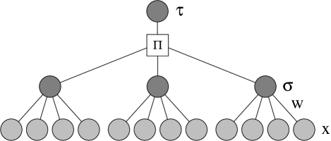
Figure 1: A tree parity machine with $K=3$ and $N=4$.

The mathematical model used in this paper is called a tree parity machine (TPM), sketched in Fig. 1. It consists of $K$ different hidden units, each of them being a perceptron with an $N$-dimensional weight vector $\mathbf{w}_{k}$. When a hidden unit $k$ receives an $N$-dimensional input vector $\mathbf{x}_{k}$ it produces the output bit

$$\sigma_{k}=\textrm{sgn}(\mathbf{w}_{k}\cdot\mathbf{x}_{k})\,.$$ (1)

The $K$ hidden units $\sigma_{k}$ define a common output bit $\tau$ of the total network by

$$\tau=\prod\limits_{k=1}^{K}\sigma_{k}\,.$$ (2)

In this paper we consider binary input values $x_{k,j}\in\{-1,+1\}$ and discrete weights $w_{k,j}\in\{-L,-L+1,...,L-1,L\}$, where the index $j$ denotes the $N$ components and $k$ the $K$ hidden units.

Each of the two communicating partners $A$ and $B$ has its own network with an identical TPM architecture. Each partner selects random initial weight vectors $\mathbf{w}_{k}^{A}(t=0)$ and $\mathbf{w}_{k}^{B}(t=0)$.

Both of the networks are trained by their mutual output bits $\tau^{A}$ and $\tau^{B}$. At each training step, the two networks receive common input vectors $\mathbf{x}_{k}$ and the corresponding output bit $\tau$ of its partner. We use the following learning rule.

1. If the output bits are different, $\tau^{A}\neq\tau^{B}$, nothing is changed.

2. If $\tau^{A}=\tau^{B}\equiv\tau$ only the hidden units are trained which have an output bit identical to the common output, $\sigma_{k}^{A/B}=\tau^{A/B}$.

3. To adjust the weights we consider three different learning rules.

   1. Anti-Hebbian learning

      $$\mathbf{w}_{k}^{+}=\mathbf{w}_{k}-\tau\mathbf{x}_{k}\Theta(\sigma_{k}\tau)\Theta(\tau^{A}\tau^{B})\,.$$ (3)

   2. Hebbian learning

      $$\mathbf{w}_{k}^{+}=\mathbf{w}_{k}+\tau\mathbf{x}_{k}\Theta(\sigma_{k}\tau)\Theta(\tau^{A}\tau^{B})\,.$$ (4)

   3. Random walk

      $$\mathbf{w}_{k}^{+}=\mathbf{w}_{k}+\mathbf{x}_{k}\Theta(\sigma_{k}\tau)\Theta(\tau^{A}\tau^{B})\,.$$ (5)

   If any component $w_{k,j}$ moves out of the interval $-L,\dots,L$, it is replaced by $\mathrm{sgn}(w_{k,j})L$.

Note that for the last rule, the dynamics of each component is identical to a random walk with reflecting boundaries. The only difference to usual random walks is that the dynamics is controlled by the $2K$ global signals $\sigma_{k}^{A/B}$ which, in turn, are determined by the ensemble of random walks. Two corresponding components of the weights of $A$ and $B$ receive an identical input $x_{k,j}$, hence they move into the same direction if the control signal allows both of them the move. As soon as one of the two corresponding components hits the boundary their mutual distance decreases. This mechanism finally leads to complete synchronization, $\mathbf{w}^{A}_{k}(t)=\mathbf{w}^{B}_{k}(t)$ for all $t\geq t_{sync}$.

On average, a common step leads to an attractive force between the corresponding weight vectors. If, however, only the weight vector of one of the two partners is changed the distance between corresponding vectors increases, on average. This may be considered as a repulsive force between the corresponding hidden units.

A learning step in at least one of the $K$ hidden units occurs if the two output bits are identical, $\tau^{A}=\tau^{B}$. In this case, there are three possibilities for a given pair of hidden units:

1. an attractive move for $\sigma_{k}^{A}=\sigma_{k}^{B}=\tau^{A/B}$;

2. a repulsive move for $\sigma_{k}^{A}\neq\sigma_{k}^{B}$;

3. and no move at all for $\sigma_{k}^{A}=\sigma_{k}^{B}\neq\tau^{A/B}$.

We want to calculate the probabilities for repulsive and attractive steps Klimov et al. (2003); Rosen-Zvi et al. (2002a). The distance between two hidden units can be defined by their mutual overlap

$$\rho_{k}=\frac{\mathbf{w}^{A}_{k}\cdot\mathbf{w}^{B}_{k}}{\sqrt{\mathbf{w}^{A}_{k}\cdot\mathbf{w}^{A}_{k}}\;\sqrt{\mathbf{w}^{B}_{k}\cdot\mathbf{w}^{B}_{k}}}\,.$$ (6)

The probability $\epsilon_{k}$ that a common randomly chosen input $\mathbf{x}_{k}$ leads to a different output bit $\sigma_{k}^{A}\neq\sigma_{k}^{B}$ of the hidden unit is given by Engel and Van den Broeck (2001)

$$\epsilon_{k}=\frac{1}{\pi}\arccos\rho_{k}\,.$$ (7)

The quantity $\epsilon_{k}$ is a measure of the distance between the weight vectors of the corresponding hidden units. Since different hidden units are independent, the values $\epsilon_{k}$ determine also the conditional probability $P_{r}$ for a repulsive step between two hidden units given identical output bits of the two TPMs. In the case of identical distances, $\epsilon_{k}=\epsilon$, one finds for $K=3$

$$P_{r} = P(\sigma^{A}_{k}\neq\sigma_{k}^{B}|\tau^{A}=\tau^{B})$$ (8)

$$= \frac{2(1-\epsilon)\epsilon^{2}}{(1-\epsilon)^{3}+3(1-\epsilon)\epsilon^{2}}\,.$$

On the other side, an attacker $E$ may use the same algorithm as the two partners $A$ and $B$. Obviously, it will move its weights only if the output bits of the two partners are identical. In this case, a repulsive step between $E$ and $A$ occurs with probability $P_{r}=\epsilon$ where now $\epsilon$ is the distance between the hidden units of $E$ and $A$.

Note that for both the partners and the attacker one has the important property that the networks remain identical after synchronization. When one has achieved $\epsilon=0$ at some time step, the distance remains zero forever, according to the previous equations for $P_{r}$. However, although the attacker uses the same algorithm as the two partners, there is an important difference: $E$ can only listen but it cannot influence $A$ or $B$. This fact leads to the difference in the probabilities of repulsive steps; the attacker has always more repulsive steps than the two partners. For small distances $\epsilon\ll 1$, the probability $P_{r}$ increases linear with the distance for the attacker but quadratic for the two partners. This difference between learning and listening leads to a tiny advantage of the partners over an attacker. The subtle competition between repulsive and attractive steps makes cryptography feasible.

On the other side, there is always a nonzero probability $P_{E}$ that an attacker will synchronize, too Mislovaty et al. (2002). For neural cryptography, $P_{E}$ should be as small as possible. Therefore it is useful to investigate synchronization for different models and to calculate their properties as a function of the model parameters.

Here we investigate a mechanism which decreases $P_{E}$, namely we include feedback in the neural networks. The input vectors $\mathbf{x}_{k}$ are no longer common random numbers, but they are produced by the bits of the corresponding hidden units. Therefore the hidden units of the two partners no longer receive an identical input, but two corresponding input vectors separate with the number of training steps. To allow synchronization, one has to reset the two inputs to common values after some time interval.

For nonzero distance $\epsilon>0$, this feedback mechanism creates a sort of noise and increases the number of repulsive steps. After synchronization $\epsilon=0$, feedback will produce only identical input vectors and the networks move with zero distance forever com .

Before we discuss synchronization and several attacking scenarios, we consider the properties of the bit sequence generated by a TPM with feedback.

III Bit Generator

We consider a single TPM network with $K$ hidden units, as in the preceding section. We start with $K$ random input vectors $\mathbf{x}_{k}$. But now, for each hidden unit $k$ and for each time step $t$, the input vector is shifted and the output bit $\sigma_{k}(t)$ is added to its first component Eisenstein et al. (1995). Simultaneously, the weight vector $\mathbf{w}_{k}$ is trained according to the anti-Hebbian rule, Eq. (3). Consequently, the bit sequence $\tau(t)$ generated by the TPM is given by the equation

$$\tau(t)=\prod\limits_{k=1}^{K}\textrm{sgn}\left(\sum\limits_{j=1}^{N}w_{k,j}(t)\sigma_{k}(t-j)\right)\,.$$ (9)

Similar bit generators were introduced in Ref. Zhu and Kinzel (1998) and the statistical properties of their generated sequences were investigated Metzler et al. (2001). Here we study the corresponding properties for our TPM with discrete weights.

The TPM network has $2^{KN}$ possible input and $(2L+1)^{KN}$ weight vectors. Therefore our deterministic finite state machine can only generate a periodic bit sequence whose length $l$ is limited by $(4L+2)^{KN}$.

Our numerical simulations show that the average length $\langle l\rangle$ of the period indeed increases exponentially fast with the size $KN$ of the network, but it is much smaller than the upper bound. For $K=3$ and $L>N$ we find $\langle l\rangle\propto(2.69)^{3N}$, independent of the number $L$ of weight values.

The network takes some time before it generates the periodic part of the sequence. We find that this transient time also scales exponentially with the system size $KN$. This means that, for sufficiently large values of $N$, say $N\geq 100$, any simulation of the bit sequence remains in the transient part and will never enter the cycle.

The bit sequence generated by a TPM with $K>2$ cannot be distinguished from a random bit sequence. For $K=L=3$ we have numerically calculated its entropy and found the value $\ln 2$ as expected from a truly random bit sequence. In addition, we have performed several tests on randomness as described by Knuth Knuth (1981). We did not find any correlations between consecutive bits; the bit sequence passed all tests on randomness within strict confidence levels.

Although the bit sequence passed many known tests on random numbers we know that it is generated by a neural network. Does this knowledge help to estimate correlations of the sequence and to predict it? In fact, for a sequence generated by a perceptron (TPM with $K=1$), another perceptron trained on the sequence could achieve an overlap to the generator Metzler et al. (2000).

Consider a bit sequence generated by a TPM with the anti-Hebbian rule. Another TPM (the “student”) is trained on this sequence using the same rule. In addition, if the output bit disagrees with the corresponding bit of the sequence, we use the geometric method of Ref. Klimov et al. (2003) to perform a training step.

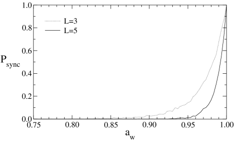
Figure 2: Probability $P_{sync}$ as a function of the fraction $a_{w}$ of initially known weights, calculated from 1000 simulations with $K=3$ and $N=100$.

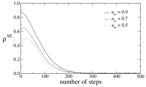
Figure 3: The average overlap between student and generator as a function of the number of steps for $K=3$, $L=5$, and $N=100$.

Figures 2 and 3 show that for $K=3$ hidden units, it is not possible to obtain an overlap to the generating TPM by learning the sequence. Only if the initial overlap between the generator and the student is very large there is a nonzero probability $P_{sync}$ that the student will synchronize with the generator. If it does not synchronize, the overlap between student and generator decays to zero.

Summarizing, a TPM network generates a pseudorandom bit sequences which cannot be predicted from part of the sequence. As a consequence, for cryptographic applications, the TPM can be used to encrypt and decrypt a secret message after it has generated a secret key.

IV Synchronization

As shown in the preceding section, a TPM cannot learn the bit sequence generated by another TPM since the two input vectors are completely separated by the feedback mechanism. This also holds for synchronization by mutual learning: With feedback, two networks cannot be attracted to an identical time dependent state. Hence, to achieve synchronization, we have to introduce an additional mechanism which occasionally resets the two inputs to a common vector. This reset occurs whenever the system has produced $R$ different output bits, $\tau^{A}(t)\neq\tau^{B}(t)$. For $R=0$ we obtain synchronization without feedback, which has been studied previously, and for large values of $R$ the system does not synchronize. Accordingly, we have added a new parameter in our algorithm which increases the synchronization time as well as the difficulty to attack the system. In the following two sections, we investigate synchronization and security of the TPM with feedback quantitatively.

We consider two TPMs $A$ and $B$ which start with different random weights and common random inputs. The feedback mechanism is defined as follows.

1. After each step $t$ the input is shifted, $x_{k,j}(t+1)=x_{k,j-1}(t)$ for $j>1$.

2. If the output bits agree, $\tau^{A}(t)=\tau^{B}(t)$, the output of each hidden unit is used as a new input bit, $x_{k,1}(t+1)=\sigma_{k}(t)$, otherwise all $K$ pairs of input bits $x_{k,1}(t)$ are set to common public random values.

3. After $R$ steps with different output, $\tau^{A}(t)\neq\tau^{B}(t)$, all input vectors are reset to public common random vectors, $x^{A}_{k,j}(t+1)=x^{B}_{k,j}(t+1)$.

Feedback creates correlations between the weights and the inputs. Therefore the system becomes sensitive to the learning rule. We find that only for the anti-Hebbian rule, Eq. (3), the components of the weights have a broad distribution. The entropy per component is larger than 99% of the maximal value $\ln(2L+1)$. For the Hebbian or random walk rule, the entropy is much smaller, because the values of the weights are pushed to the boundary values $\pm L$. Therefore the network with the anti-Hebbian rule offers less information to an attack than the two other rules.

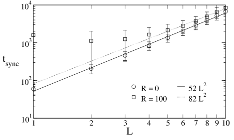
Figure 4: Average synchronization time $t_{sync}$ and its standard deviation as a function of $L$, found from 10 000 simulation runs with $K=3$ and $N=10000$. The line $52L^{2}$ is a result of linear regression for $R=0$.

In Fig. 4 we have numerically calculated the average synchronization time as a function of the number $L$ of components for the anti-Hebbian rule. Obviously, there is a large deviation from the scaling law $t_{sync}\propto L^{2}$ as observed for $R=0$. Our simulations for larger values of $N$, which are not included here, show that there exist strong finite size effects which do not allow to derive a reliable scaling law from the numerical data.

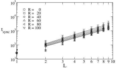
Figure 5: The synchronization time $t_{sync}$ and its standard deviation as a function of $L$, averaged over 10 000 runs of the iterative equations for $K=3$.

Fortunately, the limit $N\to\infty$ can be performed analytically. The simulation of the $KN$ weights is replaced by a simulation of an $(2L+1)\times(2L+1)$ overlap matrix $f_{a,b}^{k}$ for each hidden unit $k$ which measures the fraction of weights which are in state $a$ for the TPM $A$ and in state $b$ for $B$ Rosen-Zvi et al. (2002a, b).

We have extended this theory to the case of feedback. A new variable $\lambda_{k}(t)$ is introduced which is defined as the fraction of input components $x_{k,j}$ which are different between the corresponding hidden units of $A$ and $B$. This variable changes with time, and it influences the equation of motion for the overlap matrix $f^{k}_{a,b}(t)$. Details are described in the Appendix.

Figure 5 shows the results of this semianalytic theory. Now, in the limit of $N\to\infty$, the average synchronization time can be fitted to increase with a power of $L$, roughly proportional to $L^{2}$. The data indicate that only the prefactor but not the exponent depends on the strength $R$ of the feedback; the prefactor seems to increase linearly with $R$.

Hence, if the network is large enough, feedback has only a small effect on synchronization. In the following section we investigate the effect of feedback on the security of the network: How does the probability that an attacker is successful depend on the feedback parameter $R$?

V Ensemble of attackers

Figure 6: The success probability $P_{E}$ as a function of $L$, averaged over 10 000 simulations with $K=3$ and $N=1000$.

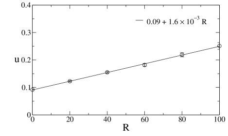
Figure 7: The coefficient $u$ as a function of the feedback parameter $R$, calculated from the results shown in Fig. 6.

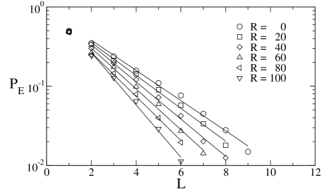
Figure 8: The success probability $P_{E}$ as a function of $L$, found from 10 000 runs of the iterative equations for $K=3$.

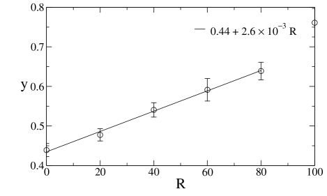
Figure 9: The coefficient $y$ as a function of the feedback parameter $R$, calculated from the results shown in Fig. 8.

Up to now, the most successful attack on neural cryptography is the geometric attack Klimov et al. (2003); Mislovaty et al. (2002). The attacker $E$ uses the same TPM with an identical training step as the two partners. That means, only for $\tau^{A}=\tau^{B}$ the attacker performs a training step. When its output bit $\tau^{E}$ agrees with the two partners, the attacker trains the hidden units which agree with the common output. For $\tau^{E}\neq\tau^{A/B}$, however, the attacker first inverts the output bit $\sigma_{k}$ for the hidden unit with the smallest absolute value of the internal field and then performs the usual training step.

For the geometric attack the probability $P_{E}$ that an attacker synchronizes with $A$ and $B$ is nonzero. Consequently, if the attacker uses an ensemble of sufficiently many networks there is a good chance that at least one of them will find the secret key.

We have simulated an ensemble of attackers using the geometric attack for the two TPMs with feedback and anti-Hebbian learning rule. Of course, each attacking network uses the same feedback algorithm as the two partner networks. Figure 6 shows the results of our numerical simulations. The success probability $P_{E}$ decreases with the feedback parameter $R$. For the model parameters shown in Fig. 6 we find that $P_{E}$ can be fitted to an exponential decrease with $L^{2}$,

$$P_{E}\propto e^{-uL^{2}}\,.$$ (10)

The coefficient $u$ increases linearly with $R$, as shown in Fig. 7. The scaling [Eq. (10)], however, is a finite size effect. For large system sizes $N$, the success probability decreases exponentially with $L$ instead of $L^{2}$,

$$P_{E}\propto e^{-yL}\,.$$ (11)

This can be seen from the limit $N\to\infty$ which can be performed with the analytic approach of the preceding section. Now the dynamics of the system is described by a tensor $f_{a,b,e}^{k}$ for the three networks $A$, $B$, and $E$ and corresponding variables $\lambda_{k}^{A},\lambda_{k}^{B},\lambda_{k}^{E}$. Details are given in the Appendix.

Figure 8 indicates the exponential scaling behavior [Eq. (11)] for several values of $R$. The coefficient $y$ increases linearly with $R$, as shown in Fig. 9.

These results show that feedback improves the security of neural cryptography. The synchronization time, on the other side, increases, too. Does the security of the system improve for constant effort of the two partners?

Figure 10: The success probability $P_{E}$ as a function of the average synchronization time $t_{sync}$, calculated from the results shown in Figs. 5 and 8.

This question is answered in Fig. 10 which shows the probability $P_{E}$ as a function of the average synchronization time, again for several values of the feedback parameter $R$. On the logarithmic scale shown for $P_{E}$, the security does not depend much on the feedback. For constant effort to find the secret key, feedback yields a small improvement of security, only.

VI Conclusions

Neural cryptography is based on a delicate competition between repulsive and attractive stochastic forces. A feedback mechanism has been introduced which amplifies the repulsive part of these forces. We find that feedback increases the synchronization time of two networks and decreases the probability of a successful attack.

The numerical simulations up to $N=10^{5}$ do not allow to derive reliable scaling laws, neither for the synchronization time nor for the success probability. But the limit $N\to\infty$ which can be performed analytically indicates that the scaling laws with respect to the number $L$ of component values are not changed by the feedback, only the respective coefficients are modified. The average synchronization time increases with $L^{2}$ while the probability $P_{E}$ of a successful attack decreases exponentially with $L$, for huge system sizes $N$.

Accordingly, the security of neural cryptography is improved by including feedback in the training algorithm. But simultaneously the effort to find the common key rises. We find that for a fixed synchronization time, feedback yields a small improvement of security, only.

After synchronization, the system is generating a pseudorandom bit sequence which passed all tests on random numbers applied so far. Even if another network is trained on this bit sequence it is not able to extract some information on the statistical properties of the sequence. Consequently, the neural cryptography cannot only generate a secret key, but the same system can be used to encrypt and decrypt a secret message, as well.

*

Appendix A Semianalytical calculation for synchronization with feedback

In this appendix we describe our extension of the semianalytic calculation Rosen-Zvi et al. (2002a, b) to the case of feedback.

The effect of the feedback mechanism depends on the fraction $\Lambda$ of newly generated input elements $x_{k,j}$ per step and hidden unit. In the numerical simulations presented in this paper $\Lambda$ is equal to $N^{-1}$. In this case the effect of the feedback mechanism vanishes in the limit $N\to\infty$. But it is also possible to generate several input elements $x_{k,j}$ per hidden unit and step. For that purpose one can multiply the output bit $\sigma_{k}$ with $\Lambda N$ random numbers $z\in\{-1,+1\}$. As we want to compare the results of the semianalytical approach with simulations for $N=1000$, we set $\Lambda=10^{-3}$ in the following calculations.

In the case of two TPMs the development of the input noise $\lambda_{k}$ is given by

$$\lambda_{k}^{+}=(1-\Lambda)\,\lambda_{k}+\Lambda\,\Theta(-\sigma_{k}^{A}\sigma_{k}^{B})\,\Theta(\tau^{A}\tau^{B})\,.$$ (12)

At the beginning and after $R$ steps with $\tau^{A}\neq\tau^{B}$ all variables $\lambda_{k}$ are set to zero (according to the algorithm described in Sec. IV).

The input noise generated by the feedback mechanism affects the output of the hidden units. An input element with $x_{k,j}^{B}=-x_{k,j}^{B}$ causes the same output $\sigma_{k}^{B}$ as a change of sign in $w_{k,j}^{B}$ together with equal inputs for both $A$ and $B$. Therefore the probability $\epsilon_{k,\mathrm{eff}}$ that two hidden units with overlap $\rho_{k}$ and input error $\lambda_{k}$ disagree on the output bit is given by

$$\epsilon_{k,\mathrm{eff}}=\frac{1}{\pi}\arccos(1-2\lambda_{k})\rho_{k}\,.$$ (13)

The distance $\epsilon_{k,\mathrm{eff}}$ between the hidden units of $A$ and $B$ is used to choose the output bits $\sigma_{k}^{A}$ and $\sigma_{k}^{B}$ with the correct probabilities in each step Rosen-Zvi et al. (2002a, b).

The feedback mechanism influences the equation of motion for the overlap matrix $f^{k}_{a,b}$, too. Here we use additional variables $\Delta_{k}^{m}=\Theta(\sigma_{k}^{m}\tau^{m})\Theta(\tau^{A}\tau^{B})$ to determine if the weights of hidden unit $k$ in the TPM of $m\in\{A,B,E\}$ change ($\Delta_{k}^{m}=1$) or not ($\Delta_{k}^{m}=0$). Therefore we are able to describe the update of elements $f_{a,b}^{k}$ away from the boundary ($-L<a,b<L$) in only one equation:

$$f^{k+}_{a,b} = \frac{1-\lambda_{k}}{2}(f^{k}_{a+\Delta_{k}^{A},b+\Delta_{k}^{B}}+f^{k}_{a-\Delta_{k}^{A},b-\Delta_{k}^{B}})$$ (14)

$$+ \frac{1}{2}\lambda_{k}(f^{k}_{a+\Delta_{k}^{A},b-\Delta_{k}^{B}}+f^{k}_{a-\Delta_{k}^{A},b+\Delta_{k}^{B}}).$$

The second term in Eq. (14) which is proportional to $\lambda_{k}$ shows the repulsive effect of the feedback mechanism. Similar equations can be derived for elements on the boundary.

In the limit $N\to\infty$ the number of steps required to achieve full synchronization diverges Kinzel and Kanter (2002a). Because of that one has to define a criterion which determines synchronization in order to analyze the scaling of $t_{sync}$ using semianalytic calculations. As in Ref. Rosen-Zvi et al. (2002a) we choose the synchronization criterion $\bar{\rho}^{AB}=\frac{1}{3}\sum_{k=1}^{K}\rho^{AB}_{k}\geq 0.9$.

In order to analyze the geometric attack in the limit $N\to\infty$ one needs to extend the semianalytical calculation to three TPMs. In this case the development of the input noise is given by the following equations:

$$\lambda_{k}^{A+} = \Lambda\,\Theta(-\sigma_{k}^{A}\sigma_{k}^{B})\,\Theta(-\sigma_{k}^{A}\sigma_{k}^{E})\,\Theta(\tau^{A}\tau^{B})$$ (15)

$$+ (1-\Lambda)\,\lambda_{k}^{A}\,,$$

$$\lambda_{k}^{B+} = \Lambda\,\Theta(-\sigma_{k}^{B}\sigma_{k}^{A})\,\Theta(-\sigma_{k}^{B}\sigma_{k}^{E})\,\Theta(\tau^{A}\tau^{B})$$ (16)

$$+ (1-\Lambda)\,\lambda_{k}^{B}\,,$$

$$\lambda_{k}^{E+} = \Lambda\,\Theta(-\sigma_{k}^{E}\sigma_{k}^{A})\,\Theta(-\sigma_{k}^{E}\sigma_{k}^{B})\,\Theta(\tau^{A}\tau^{B})$$ (17)

$$+ (1-\Lambda)\,\lambda_{k}^{E}\,.$$

Analogical to Eq. (13) the distance $\epsilon_{k,\mathrm{eff}}^{mn}$ between two hidden units can be calculated from the overlap $\rho_{k}^{mn}$ and the variables $\lambda_{k}^{m}$ and $\lambda_{k}^{n}$:

$$\epsilon_{k,\mathrm{eff}}^{mn}=\frac{1}{\pi}\arccos(1-2\lambda_{k}^{m}-2\lambda_{k}^{n})\rho_{k}^{mn}\,.$$ (18)

But for the geometric attack the attacker $E$ needs to know the local fields $h_{k}^{E}$. The joint probability distribution of $h_{k}^{A}$, $h_{k}^{B}$ and $h_{k}^{E}$ is given by Rosen-Zvi et al. (2002a)

$$P(h_{k}^{A},h_{k}^{B},h_{k}^{E})=\frac{e^{-(1/2)(h_{k}^{A},h_{k}^{B},h_{k}^{E})\mathcal{C}_{k}^{-1}(h_{k}^{A},h_{k}^{B},h_{k}^{E})^{T}}}{\sqrt{(2\pi)^{3}\det\mathcal{C}_{k}}}\,.$$ (19)

The covariance matrix in this equation describes the correlations between the three neural networks:

$$\mathcal{C}_{k}=\left(\begin{array}[]{ccc}Q_{k}^{A}&R_{k,\mathrm{eff}}^{AB}&R_{k,\mathrm{eff}}^{AE}\\ R_{k,\mathrm{eff}}^{AB}&Q_{k}^{B}&R_{k,\mathrm{eff}}^{BE}\\ R_{k,\mathrm{eff}}^{AE}&R_{k,\mathrm{eff}}^{BE}&Q_{k}^{E}\end{array}\right)\,.$$ (20)

From the tensor $f^{k}_{a,b,e}$ and the variables $\lambda_{k}^{m}$ one can easily calculate the elements of $\mathcal{C}_{k}$:

$$Q_{k}^{A} = \sum_{a,b,e=-L}^{L}{a^{2}f^{k}_{a,b,e}}\,,$$ (21)

$$Q_{k}^{B} = \sum_{a,b,e=-L}^{L}{b^{2}f^{k}_{a,b,e}}\,,$$ (22)

$$Q_{k}^{E} = \sum_{a,b,e=-L}^{L}{e^{2}f^{k}_{a,b,e}}\,,$$ (23)

$$R_{k,\mathrm{eff}}^{AB} = (1-2\lambda_{k}^{A}-2\lambda_{k}^{B})\sum_{a,b,e=-L}^{L}{abf^{k}_{a,b,e}}\,,$$ (24)

$$R_{k,\mathrm{eff}}^{AE} = (1-2\lambda_{k}^{A}-2\lambda_{k}^{E})\sum_{a,b,e=-L}^{L}{aef^{k}_{a,b,e}}\,,$$ (25)

$$R_{k,\mathrm{eff}}^{BE} = (1-2\lambda_{k}^{B}-2\lambda_{k}^{E})\sum_{a,b,e=-L}^{L}{bef^{k}_{a,b,e}}\,.$$ (26)

We use a pseudorandom number generator to determine the values of $h_{k}^{A}$, $h_{k}^{B}$, and $h_{k}^{E}$ in each step. The application of the rejection method Hartmann and Rieger (2002) ensures that the local fields have the right joint probability distribution $P(h_{k}^{A},h_{k}^{B},h_{k}^{E})$. Then the output bits $\sigma_{k}^{m}$ of the hidden units are given by $\sigma_{k}^{m}=\mathrm{sgn}(h_{k}^{m})$. If $\tau^{A}=\tau^{B}\neq\tau^{E}$ the hidden unit $k$ with the smallest absolute local field $|h_{k}^{E}|$ is searched and its output $\sigma_{k}^{E}$ is inverted (geometric attack). Afterwards the usual training of the neural networks takes place.

The equation of motion for tensor elements $f_{a,b,e}^{k}$ away from the boundary ($-L<a,b,e<L$) is given by

$$f^{k+}_{a,b,e} = \frac{1-\lambda_{k}^{A}-\lambda_{k}^{B}-\lambda_{k}^{E}}{2}\,f^{k}_{a+\Delta_{k}^{A},b+\Delta_{k}^{B},e+\Delta_{k}^{E}}$$ (27)

$$+ \frac{1-\lambda_{k}^{A}-\lambda_{k}^{B}-\lambda_{k}^{E}}{2}\,f^{k}_{a-\Delta_{k}^{A},b-\Delta_{k}^{B},e-\Delta_{k}^{E}}$$

$$+ \frac{1}{2}\lambda_{k}^{A}\,f^{k}_{a-\Delta_{k}^{A},b+\Delta_{k}^{B},e+\Delta_{k}^{E}}$$

$$+ \frac{1}{2}\lambda_{k}^{A}\,f^{k}_{a+\Delta_{k}^{A},b-\Delta_{k}^{B},e-\Delta_{k}^{E}}$$

$$+ \frac{1}{2}\lambda_{k}^{B}\,f^{k}_{a+\Delta_{k}^{A},b-\Delta_{k}^{B},e+\Delta_{k}^{E}}$$

$$+ \frac{1}{2}\lambda_{k}^{B}\,f^{k}_{a-\Delta_{k}^{A},b+\Delta_{k}^{B},e-\Delta_{k}^{E}}$$

$$+ \frac{1}{2}\lambda_{k}^{E}\,f^{k}_{a+\Delta_{k}^{A},b+\Delta_{k}^{B},e-\Delta_{k}^{E}}$$

$$+ \frac{1}{2}\lambda_{k}^{E}\,f^{k}_{a-\Delta_{k}^{A},b-\Delta_{k}^{B},e+\Delta_{k}^{E}}\,.$$

Similar equations can be derived for elements on the boundary. An attacker is considered successful if one of the conditions $\bar{\rho}^{AE}\geq 0.9$ or $\bar{\rho}^{BE}\geq 0.9$ is achieved earlier than the synchronization criterion $\bar{\rho}^{AB}\geq 0.9$.

References

- Hertz et al. (1991) J. Hertz, A. Krogh, and R. G. Palmer, Introduction to the Theory of Neural Computation (Addison Wesley, Redwood City, 1991).
- Engel and Van den Broeck (2001) A. Engel and C. Van den Broeck, Statistical Mechanics of Learning (Cambridge University Press, Cambridge, 2001).
- Metzler et al. (2000) R. Metzler, W. Kinzel, and I. Kanter, Phys. Rev. E 62, 2555 (2000).
- Kinzel et al. (2000) W. Kinzel, R. Metzler, and I. Kanter, J. Phys. A 33, L141 (2000).
- Kanter et al. (2002) I. Kanter, W. Kinzel, and E. Kanter, Europhys. Lett. 57, 141 (2002).
- Kinzel and Kanter (2003) W. Kinzel and I. Kanter, J. Phys. A 36, 11 173 (2003).
- Stinson (1995) D. R. Stinson, Cryptography: Theory and Practice (CRC Press, Boca Rotan, FL, 1995).
- Klimov et al. (2003) A. Klimov, A. Mityagin, and A. Shamir, in Advances in Cryptology - ASIACRYPT 2002, edited by Y. Zheng (Springer, Heidelberg, 2003), p. 288.
- Kinzel and Kanter (2002a) W. Kinzel and I. Kanter, in Advances in Solid State Physics, edited by B. Kramer (Springer, Berlin, 2002a), vol. 42, pp. 383–391.
- Kinzel and Kanter (2002b) W. Kinzel and I. Kanter (2002b), eprint cond-mat/0208453.
- Mislovaty et al. (2002) R. Mislovaty, Y. Perchenok, W. Kinzel, and I. Kanter, Phys. Rev E 66, 066102 (2002).
- Kanter and Kinzel (2003) I. Kanter and W. Kinzel, in Proceedings of the XXII Solvay Conference on Physics on the Physics of Communication, edited by I. Antoniou, V. A. Sadovnichy, and H. Wather (World Scientific, Singapore, 2003), p. 631.
- Rosen-Zvi et al. (2002a) M. Rosen-Zvi, E. Klein, I. Kanter, and W. Kinzel, Phys. Rev. E 66, 066135 (2002a).
- (14) A similar mechanism for a noise which increases the security of the network was recently found by combining synchronization of neural networks and chaotic maps. See Ref. Mislovaty et al. (2003).
- Mislovaty et al. (2003) R. Mislovaty, E. Klein, I. Kanter, and W. Kinzel, Phys. Rev. Lett. 91, 118701 (2003).
- Eisenstein et al. (1995) E. Eisenstein, I. Kanter, D. Kessler, and W. Kinzel, Phys. Rev. Lett. 74, 6 (1995).
- Zhu and Kinzel (1998) H. Zhu and W. Kinzel, Neural Comput. 10, 2219 (1998).
- Metzler et al. (2001) R. Metzler, W. Kinzel, L. Ein-Dor, and I. Kanter, Phys. Rev. E 63, 056126 (2001).
- Knuth (1981) D. E. Knuth, Seminumerical Algorithms, vol. 2 of The Art of Computer Programming (Addison-Wesley, Redwood City, 1981).
- Rosen-Zvi et al. (2002b) M. Rosen-Zvi, I. Kanter, and W. Kinzel, J. Phys. A 35, L707 (2002b).
- Hartmann and Rieger (2002) A. K. Hartmann and H. Rieger, Optimization Algorithms in Physics (Wiley-VCH, Berlin, 2002).