Correlations in interfering electrons irradiated by nonclassical microwaves

Abstract

Electron interference in mesoscopic devices irradiated by external non-classical microwaves, is considered. In the case of one-mode microwaves, it is shown that both the average intensity and the spectral density of the interfering electrons are sensitive to the quantum noise of the microwaves. The results for various quantum states of the microwaves are compared and contrasted with the classical case. Separable and entangled two-mode microwaves are also considered and their effect on electron average intensity and autocorrelation, is discussed.

Phys. Rev. A66, 033813 (2002).

PACS: 42.50.Dv; 85.30.St; 73.23.-b

I Introduction

Interference of electrons that encircle a magnetostatic flux has been studied for a long time since the pioneering work of Aharonov and Bohm [1]. It has applications in various contexts, for example in conductance oscillations in mesoscopic rings [2], neutron interferometry [3], and ‘which-path’ experiments [4].

A further development is the replacement of the magnetostatic flux with an electromagnetic field. In this case, the electrons feel not only the vector potential but the electromagnetic field. Therefore, the objective in this ‘ac Aharonov-Bohm’ effect is very different from the ‘dc Aharonov-Bohm’ effect (with magnetostatic flux). In the latter case the physical reality of the vector potential has been demonstrated and the subtleties of quantum mechanics in non-trivial topologies have been studied. The former case constitutes a non-linear device, where the interaction between the interfering electrons and the photons leads to interesting non-linear phenomena [5] like amplification and frequency conversion. Indeed the non-linearity can be seen in the intensity of the interfering electrons which is a sinusoidal function of the time-dependent magnetic flux. Our study is related to recent work on the interaction of mesoscopic devices with microwaves [6].

One step further in this line of work is to use in these experiments non-classical microwaves, where the quantum noise is carefully controlled. In this case, we can quantify how the quantum noise destroys slightly the electron interference [7]. More generally, we have here two coupled quantum systems (photons and electrons) and we can study how various quantum phenomena associated with the non-classical electromagnetic field cause corresponding quantum phenomena on the electrons. For example, we can study how the quantum statistics of photons affects the quantum statistics of the electrons; how the entanglement of two-mode non-classical microwaves affects the electron interference; etc.

In this paper we study how various types of non-classical microwaves affect both the average intensity and the spectral density of the interfering electrons. The results are compared with those for classical microwaves (Section II). We also consider two-mode microwaves with frequencies $\omega_{1}$ and $\omega_{2}$ in Section III, where we show that we get different results for rational and irrational values of $\omega_{1}/\omega_{2}$. We interpret these results in terms of emission and absorption of photons by the non-linear device of the interfering electrons. This discussion shows the potential use of the device for frequency conversion. Two-mode microwaves can be factorizable, separable or entangled [8]. We study how such deep quantum phenomena in the microwaves can affect the electron interference. The problem is complex and it is approached through examples which demonstrate the effect. In particular, we compare and contrast the effect on electron interference, of an entangled microwave state with that of the corresponding separable microwave state. We conclude in Section IV with a discussion of our results.

II One-mode microwaves

II.1 Classical microwaves

Interfering electric charges in mesoscopic devices that follow two different paths $C_{0}$ and $C_{1}$ are considered. A magnetic flux $\phi$ is threading the surface between the two paths. This is referred to as the dc or ac Aharonov-Bohm experiment, according to whether the magnetic flux is time-independent or time-dependent, correspondingly. In the dc Aharonov-Bohm experiment the electric charges feel only a vector potential. In the ac Aharonov-Bohm experiment the electric charges also feel an electric field, which is induced according to Faraday’s law. The ac Aharonov-Bohm effect can be realised experimentally: at low frequencies using a solenoid with a suitable time-dependent current; or at high frequencies using a waveguide, whose magnetic and electric fields are perpendicular and parallel to the plane of the two paths, respectively (Fig. 1).

Let $\psi_{0}$, $\psi_{1}$ be the electron wavefunctions with winding numbers $0,1$ correspondingly, in the absence of magnetic field. The effect of the electromagnetic field is the phase factor $\exp[ie\phi(t)]$ and the intensity is

$$I(t)=|\psi_{0}+\psi_{1}\exp[ie\phi(t)]|^{2}=|\psi_{0}|^{2}+|\psi_{1}|^{2}+2|\psi_{0}||\psi_{1}|\Re\{\exp[i(\sigma+e\phi(t))]\}$$ (1)

where $\sigma=\mbox{arg}(\psi_{1})-\mbox{arg}(\psi_{0})$. Units in which $k_{B}=\hbar=c=1$ are used throughout. For simplicity we consider the case of equal splitting, in which $|\psi_{0}|^{2}=|\psi_{1}|^{2}=1/2$ and let $\sigma=0$. In this case we get

$$I(t)=1+\cos[e\phi(t)].$$ (2)

Figure 1: ac Aharonov-Bohm phenomenon where electrons interfere in the presence of time-dependent magnetic flux (electromagnetic field). The electromagnetic field travels in the waveguide shown, with the electric field parallel to the plane of the diagram and the magnetic field perpendicular to it. The electrons follow the paths $C_{0}$, $C_{1}$ as shown.

In general, for a complex intensity $I(t)$ the autocorrelation function is defined as

$$\Gamma(\tau)=\lim_{T\rightarrow\infty}\frac{1}{2T}\int_{-T}^{T}R(t,\tau)dt;\;\;\;\;\;\;R(t,\tau)\equiv I^{*}(t)I(t+\tau).$$ (3)

The following properties of the autocorrelation function are well known:

$$\Gamma(-\tau)=\Gamma^{*}(\tau);\;\;\;\;\;\Gamma(0)\geq 0;\;\;\;\;\;|\Gamma(\tau)|\leq\Gamma(0).$$ (4)

It will be explained later that these relations are also true in the case of non-classical microwaves. The normalized autocorrelation function is defined as

$$\gamma(\tau)=\frac{\Gamma(\tau)}{\Gamma(0)};\;\;\;\;\;0\leq|\gamma(\tau)|\leq 1.$$ (5)

For one-mode microwaves, the autocorrelation function $\Gamma(\tau)$ for the charges will be periodic with a period $2\pi/\Omega$, where $\Omega$ is, by definition, the frequency associated with the periodic function $\Gamma(\tau)$. An expansion of $\Gamma(\tau)$ into a Fourier series gives the spectral density $S_{K}$:

$$S_{K} = \frac{\Omega}{2\pi}\int_{0}^{2\pi/\Omega}\Gamma(\tau)\exp(-iK\Omega\tau)d\tau$$

$$\Gamma(\tau) = \sum_{K=-\infty}^{\infty}S_{K}\exp(iK\Omega\tau).$$ (6)

Equation (4) implies that the coefficients $S_{K}$ are real numbers, for both classical and non-classical microwaves.

We consider the case where the classical time-dependent flux is given by

$$\phi(t)=\phi_{1}\sin(\omega t)$$ (7)

and using Eqs.(2),(3) we find the autocorrelation function:

$$\Gamma_{cl}(\tau)=\left[1+J_{0}(e\phi_{1})\right]^{2}+2\sum_{K=1}^{\infty}\left[J_{2K}(e\phi_{1})\right]^{2}\cos(2K\omega\tau),$$ (8)

where $J_{K}$ are Bessel functions. Comparison of Eqs.(II.1),(8) shows that $\Omega=2\omega$ and

$$S_{0}=[1+J_{0}(e\phi_{1})]^{2};\;\;\;\;\;\;S_{K}=[J_{2K}(e\phi_{1})]^{2}.$$ (9)

We note that $S_{K}=S_{-K}$. This is because in the classical case considered in this section, $I(t)$ is real and consequently $\Gamma(\tau)$ is real. Therefore Eq.(4) shows that $\Gamma(\tau)$ is an even function, which implies that $S_{K}=S_{-K}$. It is stressed that in the non-classical case considered next, $\Gamma(\tau)$ is complex in general and $S_{K}\neq S_{-K}$.

II.2 Non-classical microwaves

A monochromatic electromagnetic field of frequency $\omega$ is considered, at temperatures $k_{B}T<<\hbar\omega$. In quantized electromagnetic fields the vector potential $A_{i}$ and the electric field $E_{i}$ are dual quantum variables. For a loop $C=C_{0}-C_{1}$ (where $C_{0}$ and $C_{1}$ are the paths corresponding to 0,1 winding), which is small in comparison to the wavelength of the microwaves, the $A_{i}$ and the $E_{i}$ can be integrated around $C$ and yield the magnetic flux $\phi=\oint_{C}A_{i}dx_{i}$ and the electromotive force $V_{\rm EMF}=\oint_{C}E_{i}dx_{i}$, correspondingly, as dual quantum variables. The size of a mesoscopic device is usually of the order of $0.1\mu m$ and is indeed much smaller than the microwave wavelength. The annihilation operator is now introduced as $a=2^{-\frac{1}{2}}\xi^{-1}\left(\phi+i\omega^{-1}V_{\rm EMF}\right)$ and the corresponding creation operator, where $\xi$ is a constant proportional to the area enclosed by $C$. The flux operator is consequently written as $\phi(t)=\exp(itH)\phi(0)\exp(-itH)$, where $H$ is the Hamiltonian that contains the $\omega a^{\dagger}a$ term and an interaction term. In the ‘external field approximation’ the interaction term, which describes the back-reaction from the electrons on the electromagnetic field, is neglected. This is a good approximation for external fields which are strong in comparison to those produced dynamically by the currents in the mesoscopic device (back-reaction). In this approximation the interaction term can be ignored and we get

$$\hat{\phi}(t)=\frac{\xi}{\sqrt{2}}\left[\exp(i\omega t)a^{\dagger}+\exp(-i\omega t)a\right].$$ (10)

The phase factor $\exp(ie\phi)$ is now the operator

$$\exp\left[ie\hat{\phi}(t)\right]=D\left[iq\exp(i\omega t)\right],\ \ \ q=\frac{\xi e}{\sqrt{2}}$$ (11)

where $D(\lambda)$ is the displacement operator $D(\lambda)=\exp(\lambda a^{\dagger}-\lambda^{*}a)$. The interference between the two electron beams is described by the intensity operator

$$\hat{I}(t)=1+\cos\left[e\hat{\phi}(t)\right]=1+\frac{1}{2}D\left[iq\exp(i\omega t)\right]+\frac{1}{2}D\left[-iq\exp(i\omega t)\right].$$ (12)

Let $\rho$ be the density matrix describing the external non-classical microwaves. We can now calculate the expectation value of the electron intensity

$$\langle I(t)\rangle\equiv\mbox{Tr}\left[\rho\hat{I}(t)\right]=1+\frac{1}{2}\tilde{W}(\lambda)+\frac{1}{2}\tilde{W}(-\lambda);\ \ \ \ \lambda=iq\exp(i\omega t),$$ (13)

where $\mbox{Tr}\left[\rho D(\lambda)\right]\equiv\tilde{W}(\lambda)$ is the Weyl (or characteristic) function which has been studied by various authors including ourselves (e.g. [9] and references therein). The tilde in the notation reflects the fact that the Weyl function is related to the Wigner function through a two-dimensional Fourier transform. Physically the ${\rm Tr}\left[\rho\hat{I}(t)\right]$ describes the exchange of photons between the electrons and the external electromagnetic field. Expansion of the exponentials in Eq.(13) gives an infinite sum of terms of the type ${\rm Tr}\left[\rho(ae^{-i\omega t})^{N}(a^{\dagger}e^{i\omega t})^{M}\right]$ which describe processes in which the electrons emit $M$ photons to the external electromagnetic field and at the same time absorb $N$ photons from the external electromagnetic field. Summation of the appropriate coefficients leads to Bessel functions which appear in most of the calculations throughout the paper. We note that a similar expansion and a similar interpretation can also be made in the classical microwave case. However, in this case instead of creation and annihilation operators we have classical numbers and the interpretation is perhaps less convincing.

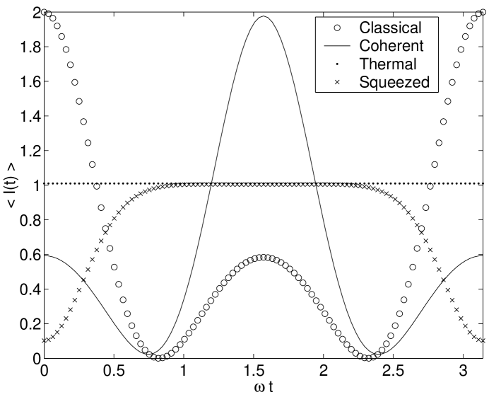
Figure 2: $\langle I(t)\rangle$ as a function of $\omega t$ for $\omega=10^{-4}$, $\langle N\rangle=100$, $r=5.5$. We use units where $\hbar=k_{B}=c=1$.

Ref.[10] has considered several density matrices and presented results for $\tilde{W}(\lambda)$. Using them we have calculated $\langle I(t)\rangle$ for various quantum states of the microwaves. We are also interested in the quantity

$$R(t,\tau)\equiv\mbox{Tr}\left[\rho\hat{I}^{\dagger}(t)\hat{I}(t+\tau)\right]$$ (14)

which is calculated for various density matrices, as well as $\Gamma(\tau)$ using Eq.(3). The Fourier series of Eq.(II.1) leads to the coefficients $S_{K}$.

We note that using the relation

$$\Gamma(\tau)=\lim_{T\rightarrow\infty}\frac{1}{2T}\int_{-T}^{T}\mbox{Tr}\left[\rho\hat{I}^{\dagger}(t)\hat{I}(t+\tau)\right]dt$$ (15)

in conjunction with the fact that for any operator $\hat{O}$, $\mbox{Tr}\left(\hat{O}^{\dagger}\right)=\left[\mbox{Tr}(\hat{O})\right]^{*}$, we prove $\Gamma(-\tau)=\Gamma^{*}(\tau)$ and therefore the coefficients $S_{K}$ are real numbers. As we already pointed out, $\Gamma(\tau)$ is in general complex. This is intimately related with the fact that the operators $\hat{I}^{\dagger}(t)$ and $\hat{I}(t+\tau)$ do not commute. In fact, the imaginary part of $R(t,\tau)$ is $(1/2)\mbox{Tr}\{\rho[\hat{I}(t),\hat{I}(t,\tau)]\}$. In the classical case, these quantities are not operators, they commute and consequently $R(t,\tau)$ is real.

II.2.1 Microwaves in coherent states

For coherent states $|A\rangle=D(A)|0\rangle$ the $R(t,\tau)$ is

$$R_{coh}(t,\tau) = 1+\exp\left(-\frac{q^{2}}{2}\right)\cos\left[2q|A|\cos(\omega t-\theta_{A})\right]$$ (16)

$$+\exp\left(-\frac{q^{2}}{2}\right)\cos\left[2q|A|\cos(\omega t+\omega\tau-\theta_{A})\right]$$

$$+\frac{1}{2}\exp\left\{-q^{2}[1+\exp(i\omega\tau)]\right\}\cos\left[4q\cos\left(\frac{\omega\tau}{2}\right)|A|\cos\left(\omega t+\frac{\omega\tau}{2}-\theta_{A}\right)\right]$$

$$+\frac{1}{2}\exp\left\{-q^{2}[1-\exp(i\omega\tau)]\right\}\cos\left[4q\sin\left(\frac{\omega\tau}{2}\right)|A|\sin\left(\omega t+\frac{\omega\tau}{2}-\theta_{A}\right)\right]$$

where $\theta_{A}=\mbox{arg}(A)$. Using Eq.(15) the electron autocorrelation function $\Gamma(\tau)$ for microwaves in coherent states is found as

$$\Gamma_{coh}(\tau) = 1+2\exp\left(-\frac{q^{2}}{2}\right)J_{0}\left(2q|A|\right)$$ (17)

$$+\frac{1}{2}\exp\left\{-q^{2}\left[1-\exp(i\omega\tau)\right]\right\}J_{0}\left[4q\sin\left(\frac{\omega\tau}{2}\right)|A|\right]$$

$$+\frac{1}{2}\exp\left\{-q^{2}\left[1+\exp(i\omega\tau)\right]\right\}J_{0}\left[4q\cos\left(\frac{\omega\tau}{2}\right)|A|\right].$$

In contrast to the case of classical microwaves, $\Gamma_{coh}(\tau)$ is now a complex function and $S_{K}\neq S_{-K}$. This is a periodic function with period $\pi/\omega$ and a Fourier series analysis is performed numerically as in Eq.(II.1).

II.2.2 Microwaves in squeezed states

Squeezed states are defined as

$$|B;r\vartheta\rangle = S(r\vartheta)|B\rangle=S(r\vartheta)D(B)|0\rangle$$ (18)

$$S(r\vartheta) = \exp\left[-\frac{r}{4}\exp(-i\vartheta)a^{\dagger 2}+\frac{r}{4}\exp(i\vartheta)a^{2}\right].$$ (19)

where $S(r\vartheta)$ is the squeezing operator. The expectation value for the electron $R_{sq}(t,\tau)$ is given by

$$R_{sq}(t,\tau) = 1+\exp(-Y_{1})\cos(X_{1})+\exp(-Y_{2})\cos(X_{2})$$ (20)

$$+\frac{1}{2}\exp\left[-iq^{2}\sin(\omega\tau)\right]\exp(-Y_{3})\cos(X_{3})$$

$$+\frac{1}{2}\exp\left[iq^{2}\sin(\omega\tau)\right]\exp(-Y_{4})\cos(X_{4})$$

where the $Y_{j}$ and $X_{j}$, are given in the Appendix. Using this result we have calculated the $\Gamma_{sq}(\tau)$ numerically. It can easily be verified that for $r=0$ the squeezed states results reduce to the coherent states results. $\Gamma_{sq}(\tau)$ is a periodic function with period $\pi/\omega$ and a Fourier series analysis is performed numerically as in Eq.(II.1).

II.2.3 Microwaves in thermal states

For thermal states, the $R(t,\tau)$ is

$$R_{th}(t,\tau) = 1+2\exp\left[-\frac{q^{2}}{2}\coth\left(\frac{\beta\omega}{2}\right)\right]$$ (21)

$$+\frac{1}{2}\exp\left[iq^{2}\sin(\omega\tau)-2q^{2}\sin^{2}\left(\frac{\omega\tau}{2}\right)\coth\left(\frac{\beta\omega}{2}\right)\right]$$

$$+\frac{1}{2}\exp\left[-iq^{2}\sin(\omega\tau)-2q^{2}\cos^{2}\left(\frac{\omega\tau}{2}\right)\coth\left(\frac{\beta\omega}{2}\right)\right]$$

and clearly $\Gamma_{th}(\tau)=R_{th}(\tau)$. The $\Gamma_{th}(\tau)$ is a periodic function with period $\pi/\omega$ and its Fourier coefficients are calculated numerically.

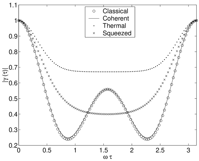
Figure 3: $|\gamma(\tau)|$ as a function of $\omega\tau$ for $\omega=10^{-4}$, $\langle N\rangle=100$, $r=5.5$. We use units where $\hbar=k_{B}=c=1$.

II.3 Results

Numerical results are presented for the four cases: classical microwaves and non-classical microwaves in coherent, squeezed and thermal states. For a meaningful comparison, we consider the case where the average number of photons $\langle N\rangle$ in coherent, squeezed and thermal states is the same:

$$\langle N\rangle=|A|^{2} = \left[\sinh\left(\frac{r}{2}\right)\right]^{2}+\left[\cosh\left(\frac{r}{2}\right)-\sinh\left(\frac{r}{2}\right)\right]^{2}B^{2}$$ (22)

$$= \frac{1}{\exp(\beta\omega)-1}.$$

For the classical case we took $\phi_{1}^{2}=2|A|^{2}=2\langle N\rangle$. In all results of Figs. 2 to 5, $\omega=10^{-4}$ (which in our units is $eV$), $\langle N\rangle=100$, $r=5.5$.

Fig. 2 shows the $\langle I(t)\rangle$ as a function of $\omega t$. In Fig. 3, the absolute value of the normalized autocorrelation function $|\gamma(\tau)|$ [Eq.(5)] is shown as a function of $\omega\tau$. The period of $|\gamma(\tau)|$ is $\pi/\omega$ (i.e., $\Omega=2\omega$) and the plots are presented from $0$ to $\pi$. As explained earlier the $\gamma(\tau)$ is real in the case of classical microwaves, but it is complex in general in the case of non-classical microwaves. This is shown explicitly in Fig. 4, which includes the imaginary parts of $\gamma(\tau)$ for all cases, as a function of $\omega\tau$. Fig. 5 shows the Fourier coefficients $S_{K}$ ($K=-2,...,2$).

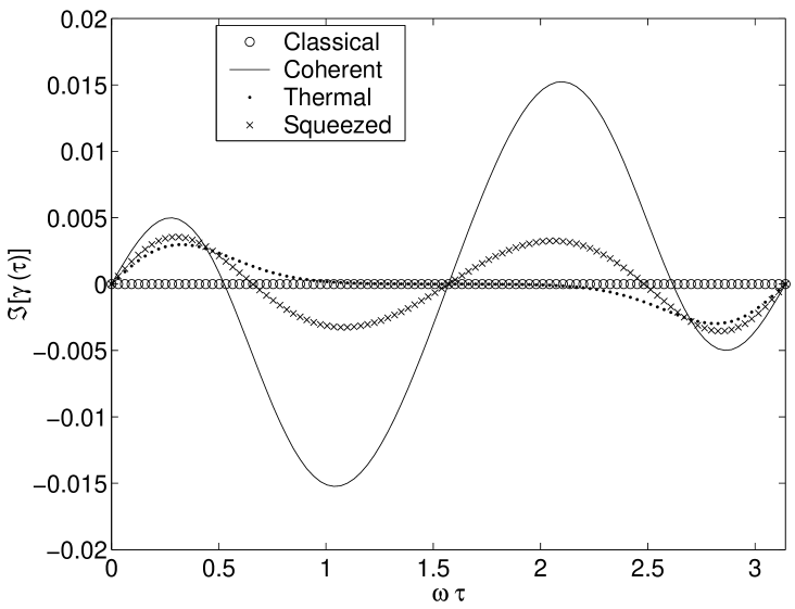
Figure 4: $\Im[\gamma(\tau)]$ as a function of $\omega\tau$ for $\omega=10^{-4}$, $\langle N\rangle=100$, $r=5.5$. We use units where $\hbar=k_{B}=c=1$.

The results quantify the effect of quantum noise on interference. All microwaves that we have considered have the same average number of photons and they differ in the quantum noise. For the classical microwaves (where the concept of number of photons is not applicable) the amplitude is equal to the amplitude of the microwaves in the coherent state. These four types of microwaves lead to different electron interference results. Fig. 2 shows clearly that $\langle I(t)\rangle$ is different in all these cases. Fig. 3 shows that the absolute normalized electron autocorrelations are different, with the exception of the classical result which is almost identical to the coherent result. The imaginary part of the electron autocorrelation (Fig. 4) distinguishes the classical from the non-classical microwave cases. It is zero for classical microwaves and takes various distinct non-zero values for different types of non-classical microwaves. The same effect can also be seen through the spectral density coefficients $S_{K}$ in Fig. 5 which are simply the Fourier transform of the electron autocorrelation function (Eq.(6)).

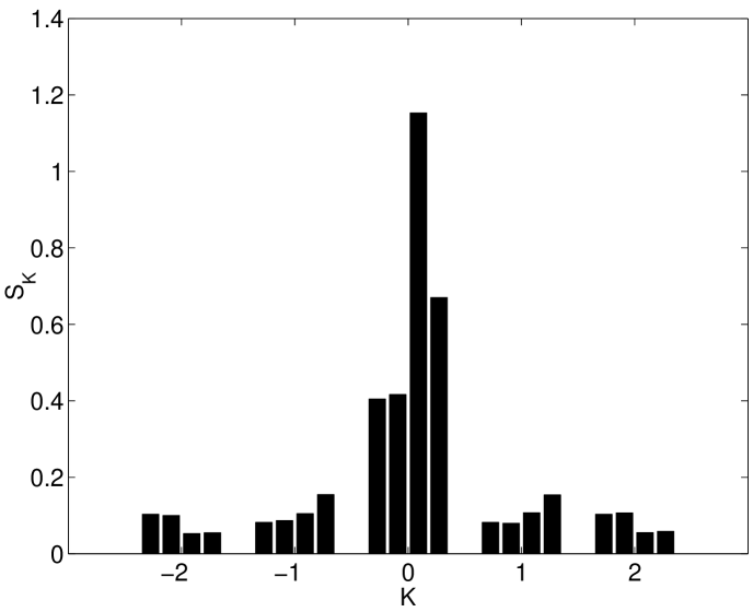
Figure 5: $S_{K}$ ($K=-2,...,2$) for $\omega=10^{-4}$, $\langle N\rangle=100$, $r=5.5$. The four columns of each value of $K$ represent from left to right classical, coherent, thermal and squeezed microwaves. We use units where $\hbar=k_{B}=c=1$.

III Two-mode microwaves

III.1 Classical microwaves

The case of classical two-mode microwaves

$$\phi(t)=\phi_{1}\sin(\omega_{1}t)+\phi_{2}\sin(\omega_{2}t).$$ (23)

is considered. In this case Eq.(2) gives the electron intensity

$$I(t)=1+\cos[e\phi_{1}\sin(\omega_{1}t)+e\phi_{2}\sin(\omega_{2}t)],$$ (24)

which is a periodic function. The autocorrelation function is different in the two cases where the ratio $\omega_{1}/\omega_{2}$ takes rational and irrational values. The physical reason for this is that in the rational case, where $\omega_{1}/\omega_{2}=P/Q$ and $P,Q$ are coprime integers, the non-linear system can act as a frequency converter by absorbing $Q$ photons of frequency $\omega_{1}$ and emitting $P$ photons of frequency $\omega_{2}$. The relation $Q\omega_{1}=P\omega_{2}$ expresses the conservation of energy. In the irrational case, the system cannot act as a frequency converter simply because there is no analogous relation for the conservation of energy.

Combining Eqs.(3),(24) it is found that in the case of irrational $\omega_{1}/\omega_{2}$, the autocorrelation is

$$\Gamma_{ir}(\tau)=1+2J_{0}(e\phi_{1})J_{0}(e\phi_{2})+\sum_{n,k=-\infty}^{\infty}\mu(\tau)\left[J_{n}(e\phi_{1})\right]^{2}\left[J_{2k-n}(e\phi_{2})\right]^{2}$$ (25)

where $\mu(\tau)=\exp\{-i[n\omega_{1}+(2k-n)\omega_{2}]\tau\}$. In the case that the ratio $\omega_{1}/\omega_{2}=P/Q$ (rational), the autocorrelation is

$$\Gamma_{ra}(\tau) = 1+\sum_{n=-\infty}^{\infty}J_{Qn}(e\phi_{1})J_{-Pn}(e\phi_{2})+\sum_{n=-\infty}^{\infty}J_{Qn}(-e\phi_{1})J_{Pn}(e\phi_{2})$$ (26)

$$+\frac{1}{4}\sum_{n,m,N=-\infty}^{\infty}\nu(\tau)J_{n}(e\phi_{1})J_{m}(e\phi_{2})J_{NQ-n}(e\phi_{1})J_{NP-m}(e\phi_{2})$$

$$+\frac{1}{4}\sum_{n,m,N=-\infty}^{\infty}\nu(\tau)J_{n}(e\phi_{1})J_{m}(e\phi_{2})J_{NQ-n}(-e\phi_{1})J_{NP-m}(-e\phi_{2})$$

$$+\frac{1}{4}\sum_{n,m,N=-\infty}^{\infty}\nu(\tau)J_{n}(-e\phi_{1})J_{m}(-e\phi_{2})J_{NQ-n}(e\phi_{1})J_{NP-m}(e\phi_{2})$$

$$+\frac{1}{4}\sum_{n,m,N=-\infty}^{\infty}\nu(\tau)J_{n}(-e\phi_{1})J_{m}(-e\phi_{2})J_{NQ-n}(-e\phi_{1})J_{NP-m}(-e\phi_{2})$$

where $\nu(\tau)=\exp[i(NQ-n)\omega_{1}\tau+i(NP-m)\omega_{2}\tau]$. It is interesting to explain the results of Eqs.(25),(26) taking into account the interpretation of the expansion of the exponentials in terms of emission/absorption of photons (discussed after Eq. (13)) in conjunction with the above comments about frequency conversion. For example, in the last term of Eq.(26) for the rational case, the system emits $n$ photons of frequency $\omega_{1}$ at time $t$ (related to an exponential $\exp(in\omega_{1}t)$); emits $NQ-n$ photons of frequency $\omega_{1}$ at time $(t+\tau)$ (related to an exponential $\exp[i(NQ-n)\omega_{1}(t+\tau)]$); absorbs $m$ photons of frequency $\omega_{2}$ at time $t$ (related to an exponential $\exp(-im\omega_{2}t)$); and absorbs $NP-m$ photons of frequency $\omega_{2}$ at time $(t+\tau)$ (related to an exponential $\exp[-i(NP-m)\omega_{2}(t+\tau)]$). Taking into account the relation $\omega_{1}/\omega_{2}=P/Q$ we see that the product of these exponentials is the factor $\nu(\tau)$. Similarly, in the last term of Eq.(25) for the irrational case the system emits $n$ photons of frequency $\omega_{1}$ at time $t$; absorbs $n$ photons of frequency $\omega_{1}$ at time $(t+\tau)$; absorbs $(2k-n)$ photons of frequency $\omega_{2}$ at time $t$; and emits $(2k-n)$ photons of frequency $\omega_{2}$ at time $(t+\tau)$. In this case there is no transfer of energy (frequency conversion) between the two frequencies. As previously, the factor $\mu(\tau)$ is related to the exponentials associated with the absorption/emission of photons. Clearly, the electron autocorrelation is a periodic function of $\tau$ only in the rational case.

III.2 Entangled two-mode microwaves

We next consider non-classical two-mode microwaves. We are particularly interested to study how entangled two-mode microwaves affect the electron interference. For this reason we consider the entangled state $|s\rangle=2^{-1/2}(|01\rangle+|10\rangle)$ where $|01\rangle$ , $|10\rangle$ are two mode number eigenstates. For comparison we also consider the separable (disentangled) state

$$\rho_{sep}=\frac{1}{2}(|01\rangle\langle 01|+|10\rangle\langle 10|).$$ (27)

Clearly, the density matrix of the entangled state $\rho_{ent}=|s\rangle\langle s|$ can be written as

$$\rho_{ent}=\rho_{sep}+\frac{1}{2}(|01\rangle\langle 10|+|10\rangle\langle 01|).$$ (28)

In this case using Eq.(13) with

$$\hat{I}(t)=1+\frac{1}{2}D_{1}(\lambda_{1})D_{2}(\lambda_{2})+\frac{1}{2}D_{1}(-\lambda_{1})D_{2}(-\lambda_{2});\ \ \ \ \lambda_{j}=iq\exp(i\omega_{j}t)$$ (29)

for two modes ($j=1,2$) we find that

$$\langle I(t)\rangle_{sep} = 1+\left(1-q^{2}\right)\exp\left(-q^{2}\right),$$ (30)

$$\langle I(t)\rangle_{ent} = \langle I(t)\rangle_{sep}-q^{2}\exp\left(-q^{2}\right)\cos[(\omega_{1}-\omega_{2})t].$$ (31)

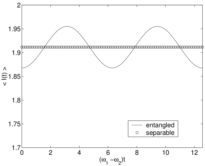
Figure 6: $\langle I(t)\rangle$ as a function of $t(\omega_{1}-\omega_{2})$ for the separable and entangled cases of Eqs.(27) and (28). We use units where $\hbar=k_{B}=c=1$.

These results are presented in Fig. 6. It is seen that for the example we considered, the $\langle I(t)\rangle_{sep}$ is constant in time, while the $\langle I(t)\rangle_{ent}$ is an oscillatory function of time. The $R(t,\tau)$ has also been calculated using Eq.(14). In the separable case, the result does not depend on $t$ and therefore

$$\Gamma_{sep}(\tau)=R_{sep}(t,\tau) = 1+\left(2-2q^{2}\right)\exp\left(-q^{2}\right)$$ (32)

$$+\frac{1}{2}\left[1-2q^{2}(s_{1}^{2}+s_{2}^{2})\right]\exp\left[iq^{2}(d_{1}+d_{2})\right]\exp\left[-2q^{2}(s_{1}^{2}+s_{2}^{2})\right]$$

$$+\frac{1}{2}\left[1-2q^{2}(c_{1}^{2}+c_{2}^{2})\right]\exp\left[-iq^{2}(d_{1}+d_{2})\right]\exp\left[-2q^{2}(c_{1}^{2}+c_{2}^{2})\right].$$

where $d_{j}=\sin(\omega_{j}\tau)$, $s_{j}=\sin(\omega_{j}\tau/2)$, $c_{j}=\cos(\omega_{j}\tau/2)$ and $j=1,2$. This is a periodic function of $\tau$ only if the ratio of $\omega_{1}/\omega_{2}$ is rational. Indeed, it can easily be verified that if $\omega_{1}/\omega_{2}=P/Q$ where $P$ and $Q$ are coprime integers, then the period is $(2\pi P)/\omega_{1}=(2\pi Q)/\omega_{2}$. The $\Gamma_{sep}(\tau)$ is a quasi-periodic function of $\tau$, if the ratio of $\omega_{1}/\omega_{2}$ is irrational. In Fig. 7 we present the absolute value of $\Gamma_{sep}(\tau)$ as a function of $\omega_{2}\tau$ for the case $\omega_{1}=1.2\times 10^{-4},\omega_{2}=10^{-4}$.

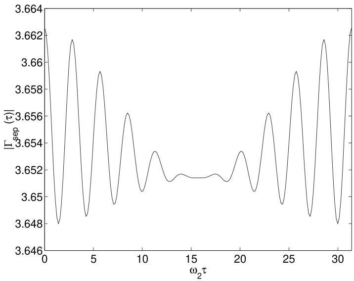
Figure 7: $|\Gamma_{sep}(\tau)|$ as a function of $\omega_{2}\tau$ for the case of Eq.(27). We use units where $\hbar=k_{B}=c=1$.

In the entangled (non-separable) microwave case

$$R_{ent}(t,\tau) = R_{sep}(t,\tau)-q^{2}\exp\left(-q^{2}\right)\cos[(\omega_{1}-\omega_{2})t]-q^{2}\exp\left(-q^{2}\right)\cos[(\omega_{1}-\omega_{2})(t+\tau)]$$ (33)

$$-2q^{2}s_{1}s_{2}\exp\left[iq^{2}(d_{1}+d_{2})\right]\exp\left[-2q^{2}(s_{1}^{2}+s_{2}^{2})\right]\cos\left[(\omega_{1}-\omega_{2})\left(t+\frac{\tau}{2}\right)\right]$$

$$-2q^{2}c_{1}c_{2}\exp\left[-iq^{2}(d_{1}+d_{2})\right]\exp\left[-2q^{2}(c_{1}^{2}+c_{2}^{2})\right]\cos\left[(\omega_{1}-\omega_{2})\left(t+\frac{\tau}{2}\right)\right]$$

With regard to the periodicity of $R_{ent}(t,\tau)$ as a function of $\tau$, similar comments can be made as for the $\Gamma_{sep}(\tau)$. We note that $R_{sep}(t,\tau)$ is independent of $t$ while $R_{ent}(t,\tau)$ is equal to $R_{sep}(t,\tau)$ plus an extra term which is a periodic function of $t$ with period $(2\pi)/(\omega_{1}-\omega_{2})$. Therefore, integration with respect to $t$ leads to the result that $\Gamma_{ent}(\tau)=\Gamma_{sep}(\tau)$.

IV Discussion

There has been a lot of work in the last few years on the interaction of mesoscopic devices with microwaves (e.g. [6]). In this paper we have considered non-classical microwaves which are carefully prepared in a particular quantum state and where the quantum noise is carefully controlled. We have studied how quantum phenomena in the microwaves, affect quantum phenomena in the interfering electrons.

We have quantified the effect of the quantum noise on electron interference. More specifically we have calculated both the average intensity and the spectral density of the interference electrons for several types of non-classical microwaves (Figs 2-5). A comparison of the results with the case of classical microwaves demonstrates clearly the influence of the quantum noise on the interference. The non-zero value of $\Im[\gamma(\tau)]$ in Fig 4 is a purely quantum mechanical result due to the non-commutativity of the quantum mechanical operators $\hat{I}(t)$ and $\hat{I}(t+\tau)$. This quantity is zero in the classical case.

We have also considered two-mode microwaves where we have shown that we get different results for rational and irrational values of the ratio $\omega_{1}/\omega_{2}$. We have interpreted these results in terms of emission and absorption of photons by the non-linear device of the interfering electrons. We have also considered both separable and entangled microwaves and quantified their effect on the interference (Figs 6-7). The different results in these two cases demonstrate how the deep quantum phenomenon of microwave entanglement affects electron interference.

V Appendix

The terms entering the squeezed states result in Eq.(20) are

$$Y_{1} = \frac{q^{2}}{2}[\cosh(r)-\sinh(r)\cos(2\omega t+\vartheta)]$$

$$X_{1} = 2q|B|\left[\cosh\left(\frac{r}{2}\right)\cos(\omega t-\theta_{B})-\sinh\left(\frac{r}{2}\right)\cos(\omega t+\theta_{A}+\vartheta)\right]$$

$$Y_{2} = \frac{q^{2}}{2}[\cosh(r)-\sinh(r)\cos(2\omega t+2\omega\tau+\vartheta)]$$

$$X_{2} = 2q|B|\left[\cosh\left(\frac{r}{2}\right)\cos(\omega t+\omega\tau-\theta_{B})-\sinh\left(\frac{r}{2}\right)\cos(\omega t+\omega\tau+\theta_{B}+\vartheta)\right]$$

$$Y_{3} = 2q^{2}\cos^{2}\left(\frac{\omega\tau}{2}\right)[\cosh(r)-\sinh(r)\cos(2\omega t+\omega\tau+\vartheta)]$$

$$X_{3} = 4q|B|\cos\left(\frac{\omega\tau}{2}\right)\left[\cosh\left(\frac{r}{2}\right)\cos\left(\omega t+\frac{\omega\tau}{2}-\theta_{B}\right)-\sinh\left(\frac{r}{2}\right)\cos\left(\omega t+\frac{\omega\tau}{2}+\theta_{B}+\vartheta\right)\right]$$

$$Y_{4} = 2q^{2}\sin^{2}\left(\frac{\omega\tau}{2}\right)[\cosh(r)+\sinh(r)\cos(2\omega t+\omega\tau+\vartheta)]$$

$$X_{4} = 4q|B|\sin\left(\frac{\omega\tau}{2}\right)\left[\cosh\left(\frac{r}{2}\right)\sin\left(\omega t+\frac{\omega\tau}{2}-\theta_{B}\right)-\sinh\left(\frac{r}{2}\right)\sin\left(\omega t+\frac{\omega\tau}{2}+\theta_{B}+\vartheta\right)\right].$$

VI References

1. Y. Aharonov and D. Bohm, Phys. Rev. 115, 485 (1959).
   A. Tonomura et. al., Phys. Rev. Lett 56, 792 (1986).
   M. Peshkin and A. Tonomura, The Aharonov-Bohm effect, Lecture notes in Physics, Vol. 340 (Springer, Berlin, 1989).

2. S. Washburn and R.A. Webb, Adv. Phys. 35, 375 (1986).
   A. G.Aronov and Y.V. Sharvin, Rev. Mod. Phys. 59, 755 (1987).
   M. Pepper, Proc. Royal Soc. London A 420, 1 (1988).

3. G. Badurek, H. Rauch, and J. Summhammer, Phys. Rev. Lett. 51, 1015 (1983).
   J. Summhammer, Phys. Rev. A 47, 556 (1993).
   J. Summhammer et al., Phys. Rev. Lett. 75, 3206 (1995).

4. A. Yacoby, M. Heiblum, D. Mahalu and H. Shtrikman, Phys. Rev. Lett. 74, 4047 (1995).
   E. Buks et. al., Nature 391, 871 (1998).
   G. Hackenbroich, Phys. Rep. 343, 464 (2001).

5. M.P. Silverman, Phys. Lett. A 118, 155 (1986); Nuovo Cimento B 97, 200 (1987).
   M. Buttiker, Phys. Rev. B 46, 12485 (1992).

6. M. Buttiker, J. Low Temp. Phys. 118, 519 (2000).
   R. Deblock et. al., Phys. Rev. B 65, 075301 (2002).

7. A. Vourdas, Phys. Rev. B 54, 13175 (1996).
   A. Vourdas and B.C. Sanders, Europhys. Lett. 43, 659 (1998).
   A. Vourdas, Phys. Rev. A 64, 053814 (2001).
   P. Cedraschi, V.V. Ponomarenko, and M. Buttiker, Phys. Rev. Lett. 84, 346 (2000).

8. R.F. Werner, Phys. Rev. A 40, 4277 (1989).
   A. Peres, Phys. Rev. Lett. 77, 1413 (1996).
   R. Horodecki and M. Horodecki, Phys. Rev. A 54, 1838 (1996).
   V. Vedral et. al., Phys. Rev. Lett. 78, 2275 (1997).

9. S. Chountasis and A. Vourdas, Phys. Rev. A 58, 848 (1998).

10. A. Vourdas, Phys. Rev. B 49, 12040 (1994).