Correlation Length Exponent in the Three-Dimensional Fuse Network

Abstract

We present numerical measurements of the critical correlation length exponent $\nu$ in the three-dimensional fuse model. Using sufficiently broad threshold distributions to ensure that the system is the strong-disorder regime, we determine $\nu$ to be $\nu=0.86\pm 0.06$ based on analyzing the fluctuations of the survival probability. The value we find for $\nu$ is very close to the percolation value $0.88$ and we propose that the three-dimensional fuse model is in the universality class of ordinary percolation.

It is already twenty years since the publication of the first experimental evidence of scaling in the morphology of brittle fractures mpp84 . About seven years later it was proposed that not only is there scaling, but the scaling properties are universal, in the sense that they do not depend on material properties blp90 ; b97 . There is now mounting evidence for this hypothesis, which may be expressed as the scaling invariance

$$\pi(z;x,y)=\lambda^{\zeta}\pi(\lambda^{\zeta}z;\lambda x,\lambda y)\;,$$ (1)

of $\pi$, which is the probability density that at position $(x,y)$ in the average fracture plane, the fracture is at height $z$ given that it is at $z=0$ at $(0,0)$, with $\zeta$ as the universal roughness exponent having a value very close to 0.80 for a large class of materials. One experimentally important consequence of this scaling is that the average fracture width $w$ scales as

$$w\sim L^{\zeta}\;,$$ (2)

where $L$ is the linear size of the average fracture plane.

Ever since the proposal of universality, it has remained a theoretical challenge to explain this value. Recently, it was suggested by Hansen and Schmittbuhl that it has its origin in the fracture process being a a correlated percolation process hs03 . The essence of the argument is based on existence of a localization length $l$ and a correlation length $\xi$ that grows during the breakdown process. The localization length depends on the disorder in the material: Stronger disorder means larger localization length. Whether the localization length diverges for large but finite disorder or it only reaches this limit for infinite disorder is at present not known. However, mean field arguments suggest that the former scenario is the correct one hhr91 . For correlation lengths $\xi$ much smaller than the localization length $l$, Hansen and Schmittbuhl hs03 assumed a relation

$$\xi\sim|p-p_{c}|^{-\nu}\;,$$ (3)

where $p$ is the local damage density and $p_{c}$ is the damage density at failure. This relation is taken directly from percolation theory. The reason it is only valid for large localization lengths $l$ is that $p$ is assumed to be spatially stationary (meaning that the statistical distribution of $p$-values is independent of position). The correlation length exponent $\nu$ has the value 4/3 in two-dimensional percolation and 0.88 in three-dimensional percolation sa92 . It is by no means given that $\nu$ should be the same in the brittle fracture problem — and Toussaint and Pride suggest that it is equal to 2 tp02 . However, it was suggested by Hansen and Schmittbuhl that the two-dimensional fuse model has $\nu=4/3$ placing it in the same universality class as two-dimensional percolation. When the correlation length approaches the localization length $l$, gradients develop in the damage — $p$ can no longer be regarded as spatially stationary — and using arguments from gradient percolation srg85 , Hansen and Schmittbuhl suggested the relation

$$\zeta=\frac{2\nu}{1+2\nu}\;.$$ (4)

With $\nu=4/3$ for the two-dimensional fuse model, this leads to $\zeta=8/11\approx 0.73$. Recent numerical calculations gives $\zeta=0.74\pm 0.03$ bbrsh03 .

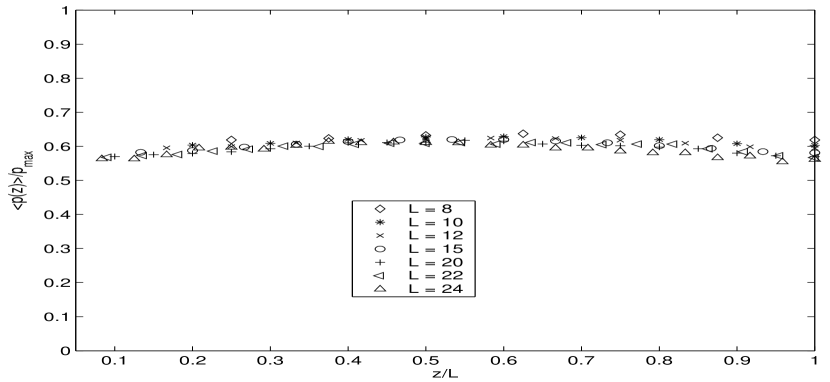
Figure 1: Normalized histogram where each bin is averaged over a plane orthogonal to the (1,1,1)-direction for $D=10$.

Recently, Kumar et al. knsz03 have proposed that there is no universal correlation length exponent $\nu$ in the two-dimensional fuse network. The numerical evidence presented is based on a disorder having a small, finite localization length so that $p$ is not spatially stationary due to localization. However, the analysis implicitly assumes that Eq. (3) is valid, which requires $p$ to be spatially stationary. Hence, there is no support for the conclusion reached.

It is the aim of this letter to measure $\nu$ in the three-dimensional fuse model. We find the value $\nu=0.86\pm 0.06$. This is close to the three-dimensional percolation value $\nu=0.88$, hence supporting the notion that the fuse model is in the universality class of ordinary percolation, both in two and three dimensions. The roughness exponent $\zeta$ was measured by Batrouni and Hansen bh98 to be $\zeta=0.62\pm 0.05$. Using Eq. (4) with $\nu=0.86$, we find $\zeta=0.63$. Hence, the value for $\nu$ we report here is consistent with the roughness exponent measured in bh98 when using Eq. (4). We note, however, that this value for the roughness exponent is not consistent with the one reported by Räisänen et al. rsad98 , who reported a roughness exponent close to the minimal energy result, $\zeta=0.41\pm 0.02$ ad96 , claiming that they should be identical.

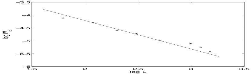
Figure 2: Log-log plot of the fluctuations of the density of broken bonds $W_{c}=(\langle p^{2}\rangle-\langle p\rangle^{2})^{1/2}$ against $L$. The disorder is hence $D$ = 10, 12, 15 and 20 respectively. The slopes are for $D=10$: 1.11, $D=12$: 1.14, $D=15$: 1.10 and $D=20$: 1.23. Their mean is $1/\nu=1.16\pm 0.06$, giving $\nu=0.86\pm 0.06$.

The fuse model that we study consists of an oriented simple cubic lattice. As in Ref. bh98 , we use periodic boundary conditions in all directions nb99 and the average current flows in the (1,1,1)-direction. Each bond is an ohmic resistor up to a threshold value. When this value is reached, the resistor turns irreversibly into an insulator. The threshold values are drawn from a spatially uncorrelated probability density $p(t)$. A voltage drop equal to unity is set up across the lattice along a given plane orthogonal to the (1,1,1)-direction. The currents are then calculated using the Conjugate Gradient algorithm bh88 . After the currents $i$ have been determined, the bond having the largest ratio $\max(i)/\max(t)$ is determined. This bond is then removed and the currents are recalculated. We do not allow the final crack to cross the plane along which the voltage drop is imposed. This simplifies the analysis of the final crack breaking the network apart, while it only imposes weak finite size corrections to fracture patterns.

The threshold values $t$ constructed by setting $t=r^{D}$, where $r$ is drawn from a uniform distribution on the unit interval bhr94 . This corresponds to a probability density $p(t)\propto t^{-1+\beta}$ on the interval $0<t<1$ with $\beta=1/D$. The parameter $D>0$ controls the width of the distribution: Larger values of $D$ corresponds to stronger disorder. In order to ensure that our results are obtained in the strong disorder phase of the fuse model, we studied $D=$ 10, 12, 15 and 20. Our system sizes varied from $L=6$ to 24 with 5000 samples generated for the smallest sizes to 200 samples for the largest sizes.

With $D=20$, the smallest threshold values generated are of the order $(24^{3})^{-20}\approx 10^{-83}$. The system has, however, still not entered purely screened percolation regime. With this level of disorder, the system fails when a fraction of about 0.62 of the bonds have failed. The threshold values of the bonds that fail near the end of the process are about $0.62^{20}\approx 10^{-4}$ — which is of the order of the currents that are carried by the bonds in the system. Hence, there is competition between threshold values and currents, making the failure process a correlated one rather than a pure percolation one even in this seemingly extreme case.

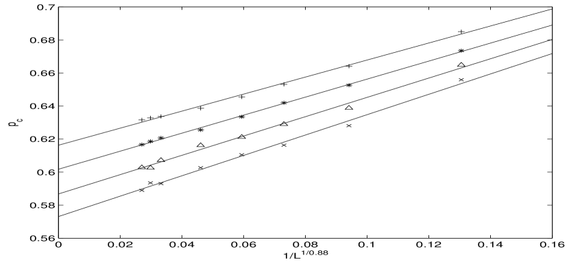
Figure 3: $\langle p\rangle$ plotted against $L^{-1/\nu}$ with $\nu=0.88$. $D=10\ (\times)$, $D=12\ (\triangle)$, $D=15\ (*)$ and $D=20\ (+)$. As $L\rightarrow\infty$ the straight lines extrapolate to the thresholds $p_{c}=0.573$, $p_{c}=0.587$, $p_{c}=0.602$ and $p_{c}=0.616$ respectively.

Fig. 1 shows the damage profile in the current direction of the random fuse model with $D=10$. We denote the (1,1,1)-direction the $z$-direction. We define the damage as the normalized average number of burned-out fuses in the plane orthogonal to the $z$-direction at $z$. The distribution has a weak maximum in the middle. This indicates a finite but large localization length $l$. Such a maximum is smaller or entirely absent from the stronger disorders (i.e. larger $D$-values) we studied.

Following percolation analysis sa92 , we define the survival probability $\Pi$ indicating the relative number of lattices that has survived for a given average damage $p$. Assuming that the disorder is broad enough so that $p$ is independent of $z$ and there is a finite critical value of $p=p_{c}$ at which 50 % of the lattices survives, we have that

$$\Pi=\Pi[(p-p_{c})L^{1/\nu}]\;.$$ (5)

This scaling ansatz implies that both the mean value of the density of broken bonds $\langle p\rangle$ and the fluctuations $(\langle p^{2}\rangle-\langle p\rangle^{2})^{1/2}$ at breakdown scales as $L^{-1/\nu}$ using

$$\langle p\rangle=\int p\biggl{(}\frac{d\Pi}{dp}\biggr{)}dp\;,$$ (6)

and

$$\langle p^{2}\rangle-\langle p\rangle^{2}=\int(p-\langle p\rangle)^{2}\biggl{(}\frac{d\Pi}{dp}\biggr{)}dp\;.$$ (7)

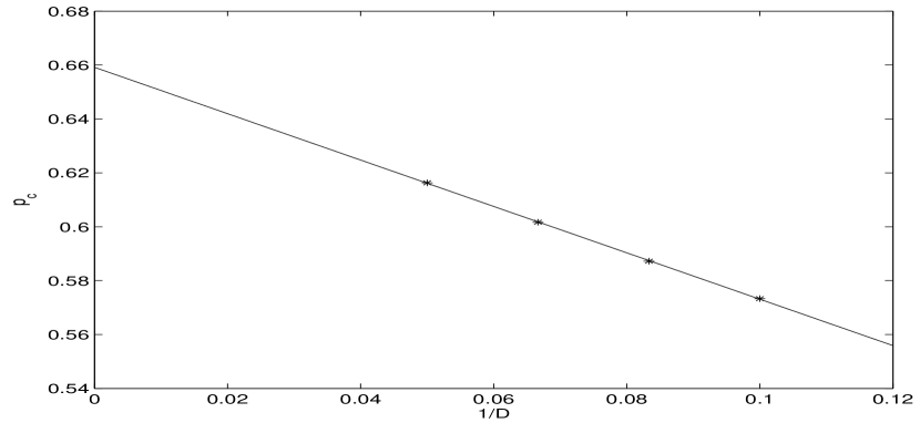
Figure 4: $p_{c}$ plotted against $1/D$ and extrapolated to infinite disorder giving $p_{c}(\infty)=0.66$. Extrapoating the straight line, towards increasing $1/D$-values, we find that $p_{c}$ becomes negative for $1/D>0.75$.

In Fig. 2 the fluctuations of the density of broken bonds, $W_{c}=\sqrt{\langle p^{2}\rangle-\langle p\rangle^{2}}$, have been plotted against the system size $L$. The mean value of the slopes gives $\nu=0.86\pm 0.06$ which is consistent with percolation value $\nu=0.88$.

Using $\nu=0.88$ from standard percolation we now turn to the scaling of $\langle p\rangle$. From finite-size scaling analysis, we expect the functional dependency

$$\langle p\rangle=p_{c}-\frac{A}{L^{1/\nu}}$$ (8)

on $L$. We show this relation for different values of $D$ in Fig. 3.

This way of measuring the critical exponent $\nu$ is much less sensitive than the one presented in Fig. 2. From standard percolation in a simple cubic lattice the threshold for an infinite system is $p_{c}=0.752$ sa92 . The extrapolations done in Fig. 4 show results lying below this threshold. However, this is to be expected as the percolation process in this limit is screened rhhg88 . This result strongly indicates that there is a strong disorder regime for finite disorders with $p_{c}$ larger than zero in the three-dimensional fuse model. In fact, extrapolating the straight line in Fig. 4 towards larger $1/D$-values will result in $p_{c}$ reaching zero and becoming negative at $D<1.33$. This is physically impossible and $p_{c}$ remains zero in this range. This indicates that there is a transition from a percolation-like regime with $p_{c}>0$ for $D>1.33$ to a regime with $p_{c}=0$ for $D<1.33$. This latter regime has been described as the diffuse localization regime in hhr91 .

In summary, we have determined the correlation length exponent in the three-dimensional fuse model to be $\nu=0.86\pm 0.06$. This is consistent with the percolation value of $\nu=0.88$. Furthermore, using Eq. (4), this is consistent with the previously measured roughness exponent $\zeta=0.62\pm 0.05$ bh98 , lending support to the scenario proposed by Hansen and Schmittbuhl hs03 for understanding the universality of the roughness exponent in the fuse model and brittle fracture. Our analysis was based on studying the fuse model with strong enough disorder for the breakdown process to develop in a percolation-like manner with $p$ spationally stationary so that the tools developed for studying that problem could be used in the present one. We note that in this regime, one will not see the fracture roughness scaling of Eq. (1): The fracture will have a fractal structure. When, on the other hand, the disorder is weak enough for localization to set in, $p$ is no longer spatially stationary, making a direct measurement of $\nu$ based on fluctuations in $p$ impossible. However, it is in this regime fracture roughness scaling as in Eq. (1) is seen as shown in bh98 .

We thank G. G. Batrouni, H. A. Knudsen, and J. Schmittbuhl for helpful discussions. B. Skaflestad is also greatly acknowledged for giving help and hints during the implementation of the numerical simulations.

References

- (1) B. B. Mandelbrot, D. E. Passoja and A. J. Paullay, Nature, 308, 721 (1984).
- (2) E. Bouchaud, G. Lapasset and J. Planès, Europhys. Lett. 13, 73 (1990).
- (3) E. Bouchaud, J. Phys. Condens. Matter, 9, 4319 (1997).
- (4) A. Hansen and J. Schmittbuhl, Phys. Rev. Lett. 90, 045504 (2003).
- (5) A. Hansen, E. L. Hinrichsen and S. Roux, Phys. Rev. B, 43, 665 (1991).
- (6) D. Stauffer and A. Aharony, Introduction to Percolation Theory (Francis and Taylor, London, 1992).
- (7) R. Toussaint and S. R. Pride, Phys. Rev. E 66, 036135 (2002); Phys. Rev. E, 66, 036136 (2002); Phys. Rev. E, 66, 036137 (2002).
- (8) B. Sapoval, M. Rosso and J. F. Gouyet, J. Phys. Lett. (France) 46, L149 (1985).
- (9) J. Ø. H. Bakke, J. Bjelland, T. Ramstad and A. Hansen, Phys. Script. T 106, 65 (2003).
- (10) P. Kumar, V. V. Nukala, S. Šimunović and S. Zapperi, Cond-Mat/0311284 (2003).
- (11) G. G. Batrouni and A. Hansen, Phys. Rev. Lett. 80, 325 (1998).
- (12) V. I. Räisänen, E. T. Seppälä, M. J. Alava and P. M. Duxbury, Phys. Rev. Lett. 80, 329 (1998).
- (13) M. J. Alava and P. M. Duxbury, Phys. Rev. Lett. 54, 14990 (1996).
- (14) M. E. J. Newman and G. T. Barkema, Monte Carlo Methods in Statistical Physics (Clarendon Press, Oxford, 1999).
- (15) G. G. Batrouni and A. Hansen, J. Stat. Phys. 52, 747 (1988).
- (16) G. G. Batrouni, A. Hansen and G. H. Ristow, J. Phys. A 27, 1363 (1994).
- (17) S. Roux, A. Hansen, H. J. Herrmann and E. Guyon, J. Stat. Phys. 52, 473 (1988).