Superfluidity of the 1D Bose gas

Superfluidité du gaz de Bose 1D

Abstract

We have investigated the superfluid properties of a ring of weakly interacting and degenerate 1D Bose gas at thermal equilibrium with a rotating vessel. The conventional definition of superfluidity predicts that the gas has a significant superfluid fraction only in the Bose condensed regime. In the opposite regime, it is found that a superfluid behaviour can still be identified when the probability distribution of the total momentum of the gas has a multi-peaked structure, revealing unambiguously the existence of ‘superfluid’ supercurrent states that did not show up in the conventional definition of superfluidity.

Résumé Cet article étudie, dans le régime d’interaction faible, les propriétés superfluides d’un gaz de Bose unidimensionnel confiné sur un anneau et à l’équilibre thermodynamique dans un référentiel tournant. La définition habituelle de la superfluidité prédit que ce gaz a une fraction superfluide appréciable seulement s’il est aussi un condensat de Bose-Einstein. Dans le régime non condensé, nous trouvons cependant qu’il est possible d’identifier un comportement superfluide en considérant la distribution de probabilité de l’impulsion totale du gaz : il existe un régime où cette distribution comporte plusieurs pics bien séparés, ce qui démontre l’existence de super-courants superfluides qui passent inaperçus dans la définition habituelle de la superfluidité.

1 Introduction

Is the weakly interacting 1D Bose gas superfluid ?

Diverging answers can be found in the literature. The Landau criterion [1] gives a positive answer, since the dispersion of elementary excitations is linear at low momenta. In the thermodynamic limit, it is argued in [2] that, on the contrary, the 1D Bose gas cannot be superfluid at finite temperature: it does not experience any phase transition, and the field correlation function vanishes exponentially at large distances, rather than with a power law. A calculation based on the Bethe ansatz, with some additional assumptions on the accessible many-body states, concludes that superfluidity is possible [3]. As shown in [4, 5] one of the subtleties of the issue is that there are actually different definitions of superfluidity, one of them based on a static (that is thermal equilibrium) property of the system, the other one involving a dynamical response of the system. In 1D, these two definitions are found to dramatically differ in the thermodynamic limit [5].

In this paper, we restrict to the strict thermal equilibrium regime, in a case where the gas can exchange momentum with a rotating vessel with walls that are smooth, at least at the macroscopic scale. Note that this differs from the usual stirring procedures used in experiments with condensates, where a macroscopic rotating defect is applied [6, 7, 8, 9]. We investigate the superfluid properties of the quantum gas in various limiting cases, from the ideal Bose gas to the weakly interacting Bose gas with weak density fluctuations, where the Bogoliubov approximation applies. We also consider an exactly solvable classical field model that allows also to study the interacting case with large density fluctuations. The applicability domain of this model has some overlap with the one of the Bogoliubov approximation, see fig.1, and in this overlap domain the two approaches give coincident results. Investigations are performed by considering not only the mean momentum of the rotating gas, but also the whole probability distribution of the total momentum: this allows to reach a much deeper physical understanding of the static aspects of the problem.

Figure 1: Scheme of the different approaches used in this paper and the corresponding applicability domains. The three temperature scales on the axis differ by a factor $(\hbar\rho/mg)^{1/2}\gg 1$ in the weakly interacting regime. ‘fluct.’ stands for ‘density fluctuations’.

2 General considerations

2.1 The physical model

Consider a one-dimensional Bose gas as described in a second-quantization approach by the Hamiltonian:

$${\mathcal{H}}_{0}=-\frac{\hbar^{2}}{2m}\int_{0}^{L}\!dx\,\hat{\Psi}^{\dagger}(x)\frac{\partial^{2}}{\partial x^{2}}\hat{\Psi}(x)+\frac{g}{2}\int\!dx\,\hat{\Psi}^{\dagger}(x)\hat{\Psi}^{\dagger}(x)\hat{\Psi}(x)\hat{\Psi}(x).$$ (1)

The $\hat{\Psi}(x)$ and $\hat{\Psi}^{\dagger}(x)$ operators are respectively the destruction and creation operators for a boson at point $x$. They obey standard bosonic commutation rules $[\hat{\Psi}(x),\hat{\Psi}^{\dagger}(x^{\prime})]=\delta(x-x^{\prime})$. The spatial coordinate $x$ runs on a ring of length $L$ with periodic boundary conditions, $m$ is the atomic mass, and the strength of local interactions is quantified by $g$. We shall restrict in this paper to the repulsive and weakly interacting case so that we impose $0<g\ll\hbar^{2}\rho/m$ [10] where $\rho$ is the mean density.

The Hamiltonian (1) is a good description of a Bose gas in a cylindrically symmetric toroidal trap [11] provided (i) the transverse trapping frequencies in the torus are much larger than both the temperature and the interaction energy per particle, $\hbar\omega_{\rho,z}\gg k_{B}T,\rho g$, and (ii) the radius $L/2\pi$ of the torus is much larger than the width of the transverse harmonic oscillator ground state which allows to neglect curvature effects in the kinetic energy. In this regime, the system is effectively 1D with periodic boundary conditions.

The gas is assumed to be at thermal equilibrium in an uniformly rotating frame, which mimics the presence of a rotating vessel containing the fluid; transfer of angular momentum from the vessel to the fluid is assumed to be possible, so that thermal equilibrium between the two can be attained. Rotation is then described by the following additional term in the Hamiltonian:

$${\mathcal{H}}_{\rm rot}=-v_{\rm rot}P,$$ (2)

where $v_{\rm rot}=\Omega L/2\pi$ is the rotation velocity and $P$ is the total momentum operator of the gas:

$$P=-i\hbar\int\!dx\,\hat{\Psi}^{\dagger}(x)\frac{\partial}{\partial x}\hat{\Psi}(x).$$ (3)

Notice that the total momentum operator $P$ gives the total mass current in the laboratory frame [12].

2.2 Definition of the normal fraction of the gas

We define the generalized normal fraction $f_{n}$ of the gas as:

$$f_{n}=\frac{\left\langle P\right\rangle}{{N}\,m\,v_{\rm rot}},$$ (4)

where the expectation value of the total momentum operator is taken in thermal equilibrium and $N$ is the total number of particles. The usual normal fraction of the gas is the limit $f_{n}^{0}$ of $f_{n}$ for $v_{\rm rot}\rightarrow 0$, and the corresponding superfluid fraction is $1-f_{n}^{0}$ [4]. For a rigid body $f_{n}=1$, which means that it is at rest in the rotating frame: the fluid is completely dragged by the walls of the rotating vessel. On the other hand $f_{n}=0$ for a pure superfluid: even if the vessel is rotating, the fluid remains at rest in the laboratory frame.

In the following sections, we shall study in detail the behaviour of $f_{n}$ for a weakly interacting one-dimensional Bose gas in different temperature and density regimes. The temperature is assumed to be always much larger than the spacing of single particle levels:

$$T\gg\frac{2\pi^{2}\hbar^{2}}{mL^{2}},$$ (5)

that is the size $L$ of the system is assumed to be much longer than the thermal de Broglie wavelength $\lambda$:

$$L\gg\lambda=\sqrt{\frac{2\pi\hbar^{2}}{mk_{B}T}}.$$ (6)

For our finite-size system, only velocity boosts $v$ which are integer multiples of the characteristic velocity:

$$v_{1}=\frac{2\pi\hbar}{mL}$$ (7)

are allowed . Galilean invariance under such boosts implies that if $\psi$ is an eigenstate of (1) of energy $E$ and momentum $P$, the boosted state $\psi^{\prime}$ is also an eigenstate of energy $E^{\prime}=E+vP+Nmv^{2}/2$ and momentum $P^{\prime}=P+Nmv$. Provided the mean number of particles $N$ is kept constant, the function $P(v_{\rm rot})$ giving the mean momentum $\left\langle P\right\rangle$ as a function of velocity $v_{\rm rot}$ therefore satisfies a periodicity condition of the form:

$$P(v_{\rm rot}+v_{1})=P(v_{\rm rot})+Nmv_{1}.$$ (9)

Because of the symmetry under spatial inversion, $P(v_{\rm rot})$ is an odd function of $v_{\rm rot}$. This property, combined with (9), implies that $P(v_{1}/2)=mNv_{1}/2$ and therefore $f_{n}(v_{1}/2)=1$. For this reason, in the following we shall restrict the definition (4) of the generalized normal fraction to the velocity range $v_{\rm rot}\in[-v_{1}/2,v_{1}/2]$.

2.3 Probability distribution of the total momentum $P$

In the previous subsection we have introduced the concept of normal fraction $f_{n}$ of the gas in terms of the expectation value of the total momentum operator $P$. We shall extend our analysis by considering not only the average value of $P$, but rather the complete probability distribution $p(P)$, which gives the probability for the total momentum to be equal to some given value $P$. Notice that this probability distribution $p(P)$ is totally different and distinct from the usual momentum distribution, which gives instead the mean number of particles in each momentum state.

As usual, the first step for the determination of $p(P)$ is the calculation of the corresponding characteristic function $g(\zeta)$:

$$g(\zeta)=\big{\langle}{e^{i\zeta P}}\big{\rangle}.$$ (10)

The probability distribution $p(P)$ is then obtained as the Fourier transform of $g$:

$$p(P)=\int\!\frac{d\zeta}{2\pi}e^{-i\zeta P}\,g(\zeta).$$ (11)

The slow rotation $v_{\rm rot}\rightarrow 0$ limit of the normal fraction can be related to the variance of $p(P)$ in the non-rotating $v_{\rm rot}=0$ system. As the total momentum $P$ commutes with the Hamiltonian ${\mathcal{H}}_{0}$, the density matrix of the fluid in the canonical ensemble at a given inverse temperature $\beta=1/k_{B}T$ can be expanded for small $v_{\rm rot}$ as:

$$\rho=e^{-\beta({\mathcal{H}}_{0}-Pv_{\rm rot})}\simeq e^{-\beta{\mathcal{H}}_{0}}\big{(}1+\beta v_{\rm rot}P\big{)}.$$ (12)

This expression can be used to calculate the expectation value of the momentum $P$ and then the small velocity limit $f_{n}^{0}$ of the normal fraction.

$$f_{n}^{0}=\lim_{v_{\rm rot}\rightarrow 0}f_{n}=\frac{\left\langle P^{2}\right\rangle}{m\,k_{B}\,T\,{N}}.$$ (13)

This relation also holds in the grand-canonical ensemble, as $P$ commutes with the number of particles and as the chemical potential $\mu$ varies only to second order in $v_{\rm rot}$ for a fixed mean number of particles. It is easy to see that for a Boltzmann gas of $N$ distinguishable and non-interacting particles, the equipartition theorem of classical statistical mechanics implies that

$$\left\langle P^{2}\right\rangle=\sum_{i}\left\langle p_{i}^{2}\right\rangle=mNk_{B}T,$$ (14)

where $p_{i}$ is the momentum of the $i$-th particle. The system is therefore totally normal $f_{n}^{0}=1$.

3 Non-interacting gas

The present section is devoted to a study of the rotational properties of a non-interacting gas. In the grand-canonical ensemble, the population of each one-particle state is described by the usual Bose distribution:

$$n_{k}=\frac{1}{e^{\beta(\epsilon_{k}-\mu)}-1},$$ (15)

where the momentum $k$ is quantized as usual as:

$$k=\frac{2\pi\hbar}{L}n,$$ (16)

$n$ being an integer, and the single-particle energy $\epsilon_{k}(v_{\rm rot})$ in the rotating frame at $v_{\rm rot}$ is equal to:

$$\epsilon_{k}(v_{\rm rot})=\frac{\hbar^{2}k^{2}}{2m}-\hbar kv_{\rm rot}.$$ (17)

The mean number of particles is

$${N}=\sum_{k}n_{k},$$ (18)

and the mean momentum is

$$\left\langle P\right\rangle=\sum_{k}\hbar k\,n_{k}.$$ (19)

The normal fraction $f_{n}$ is then immediately obtained from its definition (4). Its zero-velocity value $f_{n}^{0}$ could also be obtained from (13) by taking into account the fact that for an ideal gas one has:

$$\left\langle n_{k}^{2}\right\rangle=2\left\langle n_{k}\right\rangle^{2}+\left\langle n_{k}\right\rangle.$$ (20)

As for $v_{\rm rot}=0$ a Bose-Einstein condensate can only appear in the $k=0$ mode, the prediction for $f_{n}^{0}$ is not affected by the non-physical grand-canonical fluctuations in the condensate mode.

3.1 Non degenerate gas

In the limit $\beta\mu\rightarrow-\infty$, the occupation of all single particle modes is much smaller than unity and the Bose distribution (15) can be approximated by a Maxwell-Boltzmann law of the form:

$$n_{k}=e^{-\beta(\epsilon_{k}-\mu)}.$$ (21)

As $n_{k}$ is a slowly varying function of $k$ (the condition (5) is always assumed), one can replace the sum over $k$ in (18) and (19) by integrals $\frac{L}{2\pi}\int\!dk$. By switching to the integration variable $k^{\prime}=k+mv/\hbar$, it is then immediate to see that:

$$\left\langle P\right\rangle=m{N}v_{\rm rot},$$ (22)

which means that the fluid is completely normal and no superfluid fraction is present. Notice that this conclusion does not depend on the specific choice of the Maxwell-Boltzmann distribution (21). It rather depends on the facts that (i) the occupation number of the mode of wavevector $k$ is a function of $\hbar k-mv_{\rm rot}$ only, and (ii) sums can be replaced by integrals. Notice that the condition (i) no longer holds in the presence of interactions, which allows e.g. for superfluid behaviour of the 3D Bose gas even in the thermodynamical limit. For the ideal Bose gas, as we shall see in the next subsection, condition (ii) is violated in the Bose-condensed regime.

3.2 Classical field approximation

If one assumes that the temperature is larger than the absolute value of the chemical potential $k_{B}T\gg|\mu|$, which corresponds to the limit $\beta\mu\rightarrow 0^{-}$, the Bose distribution (15) can be approximated by the classical field one:

$$n_{k}=\frac{k_{B}T}{\epsilon_{k}-\mu}.$$ (23)

Under this approximation, analytical results can be obtained for the normal fraction $f_{n}$.

The mean density ${N}$ can be written as an infinite sum as:

$${N}=\sum_{k}\frac{k_{B}T}{\frac{\hbar^{2}k^{2}}{2m}-\hbar kv-\mu}=\frac{mL^{2}k_{B}T}{2\pi^{2}\hbar^{2}}\,\sum_{n\in{\mathbb{Z}}}\frac{1}{n^{2}-2n{\tilde{v}}+\nu^{2}},$$ (24)

where ${\tilde{v}}=v_{\rm rot}/v_{1}$ is the rescaled velocity and $\nu^{2}=-mL^{2}\mu/2\pi^{2}\hbar^{2}$. By applying the Poisson summation formula:

$$\sum_{n\in{\mathbb{Z}}}f(n)=\sum_{n\in{\mathbb{Z}}}{\hat{f}}(2\pi n),$$ (25)

where $f(x)$ is an arbitrary function and ${\hat{f}}(k)=\int dxf(x)\exp(-ikx)$ its Fourier transform, one is led to the final expression:

$${N}=\frac{mL^{2}k_{B}T}{\hbar^{2}}\,\frac{1}{2\pi\nu_{0}}\frac{\sinh(2\pi\nu_{0})}{\cosh(2\pi\nu_{0})-\cos(2\pi{\tilde{v}})},$$ (26)

where $\nu_{0}$ is defined as $\nu_{0}^{2}=\nu^{2}-{\tilde{v}}^{2}$ . By applying the same Poisson summation formula (25) to the mean momentum $\left\langle P\right\rangle$, one obtains:

$$\left\langle P\right\rangle=Nmv-\frac{mLk_{B}T}{\hbar}\,\frac{\sin(2\pi{\tilde{v}})}{\cosh(2\pi\nu_{0})-\cos(2\pi{\tilde{v}})}.$$ (27)

Notice the periodicity of ${N}$ and $\left\langle P\right\rangle$ as functions of the reduced velocity ${\tilde{v}}$. This in agreement with the general result (9). From (26) and (27) we immediately obtain the generalized normal fraction:

$$f_{n}=\frac{\left\langle P\right\rangle}{{N}mv}=1-\frac{\nu_{0}}{{\tilde{v}}}\,\frac{\sin(2\pi{\tilde{v}})}{\sinh(2\pi\nu_{0})}.$$ (28)

The physics of the non-interacting classical field is determined by the dimensionless parameter $\nu$ and the rotation velocity ${\tilde{v}}$. For a given rotation velocity $v_{\rm rot}$, the crossover from $\nu\gg 1$ to $\nu\ll 1$ corresponds to the Bose condensation in the finite system. In the high density $\nu\rightarrow 0$ limit where the gas is fully Bose-condensed, one has $\nu_{0}\rightarrow i{\tilde{v}}$ and the normal fraction (28) tends to zero. On the other hand, for $\nu\rightarrow\infty$, $\nu_{0}\rightarrow\infty$ and the normal fraction consequently tends to $1$.

In the absence of rotation ${\tilde{v}}=0$, Bose condensation in the finite system occurs for [13]:

$$k_{B}T\approx k_{B}T_{\rm BEC}=\frac{6N\hbar^{2}}{mL^{2}},$$ (29)

that is when the coherence length $l_{c}=\rho\lambda^{2}/2\pi$ of the gas becomes larger than the size $L$ of the system. Even in this zero-velocity case, the normal fraction

$$f_{n}^{0}=1-\frac{2\pi\nu_{0}}{\sinh(2\pi\nu_{0})}$$ (30)

differs from the non-condensed one $f_{\rm nc}$:

$$f_{\rm nc}=\frac{{N}-\left\langle n_{k=0}\right\rangle}{{N}}=1-\frac{\cosh(2\pi\nu_{0})-1}{\pi\nu_{0}\sinh(2\pi\nu_{0})}.$$ (31)

In particular, in the limit of a well-established Bose-Einstein condensate $\nu_{0}\ll 1$, one has the peculiar relation:

$$f_{n}^{0}=2f_{\rm nc},$$ (32)

which states that the normal fraction is twice as large than the non-condensed one, and, therefore, that the condensate is not completely superfluid. This prediction is qualitatively opposite to what is found in liquid ⁴He, which at low temperatures is totally superfluid even if the condensate fraction is only of the order of 10% [14, 15].

3.3 Probability distribution of the total momentum

For the ideal Bose gas, the total momentum is simply written in terms of the single-particle occupation numbers $n_{k}$ as $P=\sum_{k}\hbar k\,n_{k}$, so the characteristic function $g_{p}$ is equal to:

$$g(\zeta)=\left\langle e^{iz\sum_{k}\hbar k\,n_{k}}\right\rangle=\prod_{k}\left\langle e^{i\zeta\hbar k\,n_{k}}\right\rangle=\prod_{k}\frac{1-e^{-\beta(\epsilon_{k}-\mu)}}{1-e^{-\beta(\epsilon_{k}-\mu)}\,e^{i\zeta\hbar k}},$$ (33)

which has a factorized form over single particle states. In the classical field approximation, this infinite product can be calculated exactly, as shown in section 5.

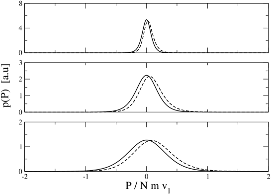
Figure 2: Probability distribution $p(P)$ of the total momentum $P$ for an ideal Bose gas of $1000$ particles. Rotation velocity $v_{\rm rot}=0$ (solid lines), $v_{\rm rot}/v_{1}=0.125$ (dashed lines). Temperatures $T/(Nmv_{1}^{2}/2)=0.05,0.125,0.25$ (from top to bottom: the corresponding normal fractions are respectively: $f_{n}=0.3,0.64,0.92$).

The probability distribution $p(P)$ without the classical field approximation is easily obtained by numerical Fourier transform of (33) (fig.2). For a vanishing $v_{\rm rot}$ , the distribution $p(P)$ is simply narrowed as the temperature is decreased and no additional structure appears. An analytical proof of the fact that $p(P)$ has a single maximum for $v_{\rm rot}=0$ is given in the appendix A in the classical field approximation. Superfluidity effects can therefore be seen only as a more rapid shrinking of the distribution as compared to the case of a normal gas (cf. (13)). For a slow but finite rotation speed $v_{\rm rot}<v_{1}/2$, the flow of particles simply appears as a shift-like distortion in the probability distribution .

4 Interacting gas I: multi-valley Bogoliubov approach

The present section is devoted to the calculation of the rotational properties of a weakly interacting Bose gas at temperatures low enough for density fluctuations to be weak. In this regime, the Bogoliubov theory can be used to describe the system. Since we are dealing with one-dimensional systems in which no long-range order is present for the phase of the Bose field, the extension of the Bogoliubov theory to quasi-condensates with only a finite-range order should be used, as discussed in [16]. For simplicity we shall use the version of the method in the canonical ensemble.

Quantitatively, the weakly interacting gas condition can be written in terms of the density $\rho=N/L$ and the healing length $\xi$ as [10]:

$$\rho\xi=\sqrt{\frac{\hbar^{2}\rho}{mg}}\gg 1,$$ (34)

while the weakness of density fluctuations $\Delta\rho/\rho\ll 1$ requires [16]:

$$k_{B}T\ll k_{B}T_{\rm df}=\rho g\times\rho\xi=\Big{(}\frac{\hbar^{2}}{m}\rho^{3}g\Big{)}^{1/2}.$$ (35)

In the weakly interacting regime (34), $T_{\rm df}$ is always much lower than the temperature

$$T_{\rm deg}=2\pi\hbar^{2}\rho^{2}/m$$ (36)

for quantum degeneracy.

4.1 Mean total momentum in the Bogoliubov approximation

The preliminary step to the Bogoliubov approach is to use the pure quasi-condensate approximation and identify the quasi-condensate wavefunction $\phi_{0}(x)$ as a local minimum of the Gross-Pitaevskii energy functional:

$$E_{GP}[\phi]=\int\!dx\,\left[\frac{\hbar^{2}}{2m}|\partial_{x}\phi|^{2}+\frac{Ng}{2}|\phi|^{4}+i\hbar v_{\rm rot}\phi^{*}\partial_{x}\phi\right].$$ (37)

A local minimum has to be a stationary state of the Gross-Pitaevskii equation

$$\mu\phi=\left[-\frac{\hbar^{2}}{2m}\partial_{x}^{2}+Ng|\phi|^{2}+i\hbar v_{\rm rot}\partial_{x}\right]\phi.$$ (38)

Here we take for stationary states the usual form of plane waves:

$$\phi_{0}(x)=\frac{1}{\sqrt{L}}e^{ik_{0}x}.$$ (39)

The periodic boundary conditions impose that the momentum is quantized as $k_{0}=2\pi w_{0}/L$, $w_{0}$ being an integer called the winding number. The corresponding velocity $v_{0}=w_{0}v_{1}$ will be called in the following quasi-condensate velocity. The chemical potential is then

$$\mu=g\rho+\frac{1}{2}m\,v_{0}^{2}-m\,v_{0}\,v_{\rm rot}.$$ (40)

The resulting energy of the pure quasi-condensate is then:

$$E_{GP}[v_{\rm rot},v_{0}]=N\Big{[}\frac{1}{2}m\,v_{0}^{2}-m\,v_{0}\,v_{\rm rot}\Big{]}+\frac{1}{2}N\rho g.$$ (41)

Under the low-temperature and weak-interaction conditions stated above, the fluctuations of the Bose field around the pure quasi-condensate field can be described by the Bogoliubov Hamiltonian [16, 17]:

$${\mathcal{H}}_{\rm Bog}=E_{GP}[v_{\rm rot},v_{0}]-\sum_{k\neq 0}\epsilon_{k}\,V_{k}^{2}+\sum_{k\neq 0}\epsilon_{k}\hat{b}^{\dagger}_{k}\hat{b}_{k},$$ (42)

where the $\hat{b}_{k},\hat{b}^{\dagger}_{k}$ operators are the usual (bosonic) destruction and creation operators for the Bogoliubov quasi-particles. Their dispersion relation $\epsilon_{k}(v_{\rm tot},v_{0})$ is given by:

$$\epsilon_{k}(v_{\rm rot},v_{0})=\epsilon^{0}_{k}+\hbar k(v_{0}-v_{\rm rot})$$ (43)

in terms of the usual dispersion relation $\epsilon^{0}_{k}$ for a system at rest ($v_{0}=v_{\rm rot}=0$):

$$\epsilon^{0}_{k}=\Big{[}\frac{\hbar^{2}k^{2}}{2m}\big{(}\frac{\hbar^{2}k^{2}}{2m}+2\rho g\big{)}\Big{]}^{1/2}.$$ (44)

The $V_{k}$ coefficients are defined as:

$$V_{k}=\frac{1}{2}\Big{(}\Big{[}\frac{\frac{\hbar^{2}k^{2}}{2m}}{\frac{\hbar^{2}k^{2}}{2m}+2\rho g}\Big{]}^{1/4}-\Big{[}\frac{\frac{\hbar^{2}k^{2}}{2m}+2\rho g}{\frac{\hbar^{2}k^{2}}{2m}}\Big{]}^{1/4}\Big{)}.$$ (45)

The fact that the $V_{k}$ do not depend on $v_{0}-v_{\rm rot}$ is a consequence of Galilean invariance. One has also to calculate the total momentum operator (3):

$$P=Nmv_{0}+\sum_{k\neq 0}\hbar k\,\hat{b}_{k}^{\dagger}\hat{b}_{k}.$$ (46)

The fact that the total number of particles enters in the first term of the righthand side of this equation (rather than the number of particles in the quasi-condensate or the number of particles in the superfluid fraction) is again a consequence of Galilean invariance. A derivation of ${\mathcal{H}}_{\rm Bog}$ and $P$ is given in the appendix B.

The quasi-condensate mode $\phi_{0}(x)$ is a local minimum of the Gross-Pitaevskii energy functional if all the $\epsilon_{k}$ are positive, which guarantees the thermodynamical stability of the gas. This condition can be reformulated as:

$$|v_{0}-v_{\rm rot}|\leq\textrm{min}_{k\neq 0}\Big{[}\frac{\epsilon^{0}_{k}}{\hbar k}\Big{]}.$$ (47)

When the length $L$ is larger than the healing length $\xi$, this criterion reduces to the usual Landau criterion which states that the flow velocity as measured in the moving frame has to be smaller than the sound velocity $c=(\rho g/m)^{1/2}$ of the gas at rest.

A key assumption of our multi-valley Bogoliubov approach is that the density matrix of the system is a statistical mixture of states of different winding numbers $w_{0}$ and thus quasi-condensate velocities $v_{0}=w_{0}v_{1}$. Each value of $v_{0}$ corresponds to a separate minimum – a valley – of the Gross-Pitaevskii energy functional (37) and the fluctuations around each of them are treated within the Bogoliubov approximation previously discussed.

The expectation value of any observable, e.g. the momentum $P$, is then expressed as an average over the different valleys:

$$\left\langle P\right\rangle=\frac{1}{{\mathcal{Z}}_{T}}\sum_{v_{0}}{\mathcal{Z}}_{v_{0}}\,\left\langle P\right\rangle_{v_{0}}.$$ (48)

Obviously, only stable states satisfying (47) are to be taken into account. The ${\mathcal{Z}}_{v_{0}}$ are the contributions of the different valleys to the total partition function:

$${\mathcal{Z}}_{v_{0}}=\textrm{Tr}[e^{-\beta{\mathcal{H}}}]_{v_{0}}=A\;e^{-\frac{1}{2}\beta Nm(v_{0}-v_{\rm rot})^{2}}\prod_{k\neq 0}\frac{1}{1-e^{-\beta\epsilon_{k}(v_{\rm rot},v_{0})}},$$ (49)

where $A$ is a overall factor which does not depend on $w_{0}$ and therefore drops out from all the calculations that follow. The total partition function is ${\mathcal{Z}}_{T}=\sum_{v_{0}}{\mathcal{Z}}_{v_{0}}$.

The expectation value of $P$ within a given valley $\langle P\rangle_{v_{0}}$ is obtained as the thermal average of (46):

$$\langle P\rangle_{v_{0}}=Nmv_{0}+\sum_{k\neq 0}\frac{\hbar k}{\exp\{-\beta[\epsilon_{k}^{0}-\hbar k(v_{\rm rot}-v_{0})]\}-1}\equiv Nmv_{0}+Nm(v_{\rm rot}-v_{0})\;f_{n}^{v}(v_{\rm rot}-v_{0}).$$ (50)

The function $f_{n}^{v}(v)$ has a very simple physical interpretation: it is the generalized normal fraction of the gas that one would predict in a single valley Bogoliubov treatment (i.e. winding number $w_{0}=0$) for a rotation velocity $v$. Hence the superscript $v$.

In the remaining part of this section we shall restrict to the case

$$L\gg\xi.$$ (51)

This will provide a considerable simplification of the expression of $\langle P\rangle$.

First because this allows to replace in $f_{n}^{v}(v)$ the sum over $k$ by an integral. The resulting integral may be calculated in the limit of low and high temperatures. If the temperature is sufficiently low:

$$k_{B}T\ll\rho g\Big{(}1-\Big{|}\frac{v}{c}\Big{|}\;\Big{)},$$ (52)

only the linear part of the spectrum effectively contributes to the integral. This leads to

$$f_{n}^{v}(v)=\frac{(k_{B}T)^{2}}{c^{3}}\frac{\pi}{3m\hbar\rho}\frac{1}{(1-{v^{2}}/{c^{2}})^{2}},$$ (53)

where $c=\sqrt{{\rho g}/{m}}$ is the sound velocity.

For temperatures $k_{B}T\gg\rho g$ but still smaller than the temperature $T_{\rm df}$ at which density fluctuations becomes important, a classical field approximation can be performed on the Bose distribution law, which leads to

$$f_{n}^{v}(v)=\frac{k_{B}T}{\hbar c\rho}\frac{1}{\sqrt{1-{v^{2}}/{c^{2}}}}.$$ (54)

Within their own domain of validity, both (53) and (54) predict a single-valley normal fraction much smaller than one.

Let us assume that $|v_{\rm rot}-v_{0}|\ll c$ for all the relevant terms in the sum (48). In this case, (50) can be simplified as follows:

$$\langle P\rangle_{v_{0}}\simeq Nmf_{n}^{v,0}v_{\rm rot}+Nmv_{0}(1-f_{n}^{v,0}),$$ (55)

where $f_{n}^{v,0}$ is the zero-rotation limit of $f_{n}^{v}$:

$$f_{n}^{v,0}=f_{n}^{v}(0)=\frac{1}{Nmk_{B}T}\sum_{k\neq 0}(\hbar k)^{2}\frac{e^{\beta\epsilon_{k}^{0}}}{(e^{\beta\epsilon_{k}^{0}}-1)^{2}}.$$ (56)

The result (55) can be physically understood in the following terms: for any value of the quasi-condensate velocity $v_{0}$, the normal fraction $f_{n}^{v,0}$ within the valley is moving at a rotation velocity $v_{\rm rot}$, while the superfluid fraction $1-f_{n}^{v,0}$ moves independently at $v_{0}$.

In this limit $|v_{\rm rot}-v_{0}|\ll c$, the expression (49) for the partial partition function for each valley can be simplified by expanding the product to second order in $v_{\rm rot}-v_{0}$:

$$\prod_{k\neq 0}\frac{1}{1-e^{-\beta\epsilon_{k}(v_{\rm rot},v_{0})}}\simeq e^{\frac{1}{2}\beta Nmf_{n}^{v,0}(v_{\rm rot}-v_{0})^{2}}\prod_{k\neq 0}\frac{1}{1-e^{-\beta\epsilon^{0}_{k}}}.$$ (57)

By inserting this expression into (49), the final expression for the expectation value of the momentum (48) gets the simple form:

$$P(v_{\rm rot})=f_{n}^{v,0}Nmv_{\rm rot}+N(1-f_{n}^{v,0})\,\sum_{v_{0}}q(v_{0})\,mv_{0},$$ (58)

in which the normal gas always moves at a velocity $v_{\rm rot}$ and the probability distribution $q(v_{0})$ for the quasi-condensate to have a velocity $v_{0}$ has the Gaussian form:

$$q(v_{0})={\mathcal{N}}_{q}\,\exp\Big{[}-\frac{mN(1-f_{n}^{v,0})}{2k_{B}T}\big{(}v_{\rm rot}-v_{0}\big{)}^{2}\Big{]},$$ (59)

where ${\mathcal{N}}_{q}$ is the normalization factor. Note that only the fraction $1-f_{n}^{v,0}$ of atoms which are superfluid in a single valley treatment is actually involved in (59). The normal fraction of the gas can be obtained from (58):

$$f_{n}^{0}=f_{n}^{v,0}+\frac{Nm(1-f_{n}^{v,0})^{2}}{k_{B}T}\frac{\sum_{v_{0}}v_{0}^{2}\exp\Big{[}-\frac{1}{2}\beta mN(1-f_{n}^{v,0})\,v_{0}^{2}\Big{]}}{\sum_{v_{0}}\exp\Big{[}-\frac{1}{2}\beta mN(1-f_{n}^{v,0})\,v_{0}^{2}\Big{]}}.$$ (60)

Remarkably this expression coincides with formula (11) of [5] if one takes $\rho_{S}=(1-f_{n}^{v,0})\rho$ in [5].

We briefly come back to the condition $|v_{\rm rot}-v_{0}|\ll c$. For $v_{0}=0$, this hypothesis is a direct consequence of (51) since $v_{\rm rot}$ can be taken in the interval $[-v_{1}/2,v_{1}/2]$. What happens if $v_{0}\gg v_{1}$? The maximal accessible value $v_{0}^{\rm max}$ of $v_{0}$ allowed by the probability distribution (59) corresponds to $mv_{0}^{2}/2\approx k_{B}T/N$. $v_{0}^{\rm max}$ is much smaller than $c$ provided $k_{B}T\ll N\rho g$. As:

$$\frac{k_{B}T}{N\rho g}=\frac{T}{T_{\rm df}}\frac{\xi}{L},$$ (61)

this is automatically satisfied since we have assumed $L\gg\xi$ and $T\ll T_{\rm df}$.

Even if the normal fraction $f_{n}^{v,0}$ within a single valley is always small $f_{n}^{v,0}\ll 1$ in the regime of validity of the Bogoliubov approximation, the true normal fraction tends to one as soon as several valleys are thermally populated

$$k_{B}T\geq k_{B}T_{v}=\frac{1}{2}Nmv_{1}^{2}.$$ (62)

In this case, one can replace the discrete sum over $v_{0}$ by an integral in (58):

$$\langle P\rangle\simeq Nmv_{\rm rot},$$ (63)

finding that the transport of atoms in the presence of a finite $v_{\rm rot}$ is essentially due to the redistribution of the population among the different valleys. In other words, as several different values of the quasi-condensate velocity $v_{0}$ are accessible, the presence of a finite rotation velocity causes an imbalance of the relative probabilities $q(v_{0})$ and therefore a net matter flow.

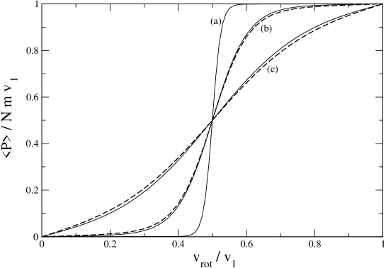
Figure 3: Average value of the total momentum $P$ as a function of the rotation velocity $v_{\rm rot}$ for a Bose gas of $1000$ interacting atoms. Chemical potential $\rho g/k_{B}T_{v}=0.1$. Temperatures: $T/T_{v}=0.025$ (a), $0.1$ (b), $0.25$ (c). Solid lines: many-valley Bogoliubov predictions. Dashed lines for (b) and (c): full numerical solution of the classical field model of section 5. For curve (a), $k_{B}T=\rho g/4\ll\rho g$, outside the applicability range of the classical field model.

The Bogoliubov prediction for $\langle P\rangle$ as function of $v_{\rm rot}$ is plotted in figure 3 for various values of the temperature. In the low temperature regime $T\ll T_{v}$, only the valley with $w_{0}=0$ is generally occupied for $v_{\rm rot}<v_{1}/2$: the full normal fraction is close to the single valley prediction, so that the gas is almost fully superfluid. When $v_{\rm rot}$ approaches $v_{1}/2$, the valleys $w_{0}=0$ and $w_{0}=1$ become nearly degenerate: the Gross-Pitaevskii energies (41) of a condensate at rest $v_{0}=0$ and in the first excited state $v_{0}=v_{1}$ are nearly equal. In this case, even if $T\ll T_{v}$, both valleys can be populated and their relative weights will be strongly dependent on $v_{\rm rot}$, see the step function in figure 3. For $v_{\rm rot}>v_{1}/2$, only the valley $w_{0}=1$ is occupied. The width of the crossover from a value $\langle P\rangle\ll Nmv_{\rm rot}$ to a value $Nmv_{\rm rot}-\langle P\rangle\ll Nm(v_{1}-v_{\rm rot})$ is of the order of

$$\Delta v_{\rm rot}=\frac{k_{B}T}{Nmv_{1}}.$$ (64)

In the opposite regime of a temperature on the order of $T_{v}$, where several valleys are thermally populated, the step behaviour of $P(v_{\rm rot})$ is smoothed out and the gas become normal, as predicted in (63).

4.2 Comparison with Quantum Monte Carlo simulation

The predictions of the many-valley Bogoliubov approach can be verified against a Quantum Monte Carlo calculation performed using a recently developed stochastic field technique for the interacting Bose gas [18]. As rotation is described by an additional single-particle term $-Pv_{\rm rot}$ in the Hamiltonian, the numerical simulation does not present any further complication with respect to the ones previously performed, e.g. for the study of the statistical properties of a Bose-Einstein condensate [19].

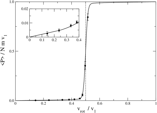
Figure 4: Average value of the total momentum $P$ as a function of the rotation velocity $v_{\rm rot}$ for a 1D Bose gas of $42$ interacting atoms. Chemical potential $\rho g/k_{B}T_{v}=0.017$, $T/T_{v}=0.017$. Solid line: many-valley Bogoliubov theory. Points: Quantum Monte Carlo calculation.

In fig.4 we have compared the result of the Monte Carlo simulation with the prediction of the many-valley Bogoliubov theory. As the condition $L\gg\xi$ is not fulfilled, a numerical evaluation of (48-50) is necessary. The parameters of the figure correspond to a regime in which only a single valley is thermally populated $T\ll T_{v}$: the agreement is good in the slow-velocity regime $v_{\rm rot}\ll v_{1}$ as well as close to the point $v_{\rm rot}=v_{1}/2$ where the two valleys of winding numbers respectively $w_{0}=0$ and $w_{0}=1$ become degenerate and the system is in a statistical mixture of them.

4.3 Probability distribution of the total momentum

If the temperature is sufficiently low for density fluctuations to be small, the many-valley Bogoliubov theory introduced in the previous subsection can be used to calculate not only the normal fraction but also the complete probability distribution $p(P)$ for the total momentum $P$.

Using the expression (46) of the total momentum operator in the Bogoliubov approximation, the characteristic function $g(\zeta)$ can be written as:

$$g(\zeta)=\frac{1}{{\mathcal{Z}}_{T}}\sum_{v_{0}}{\mathcal{Z}}_{v_{0}}e^{i\zeta Nmv_{0}}\left\langle e^{i\zeta\sum_{k}\hbar kn_{k}}\right\rangle_{v_{0}}=\frac{1}{{\mathcal{Z}}_{T}}\sum_{v_{0}}e^{-\frac{1}{2}\beta Nm(v_{0}-v_{\rm rot})^{2}}e^{i\zeta Nmv_{0}}\prod_{k}\frac{1}{1-e^{-\beta[\epsilon_{k}^{0}-\hbar k(v_{\rm rot}-v_{0})]}e^{i\zeta\hbar k}},$$ (65)

where $n_{k}$ are now the occupation numbers of the Bogoliubov quasi-particle modes of energies $\epsilon_{k}$.

It is apparent in the last factor of (65) that the presence of $\zeta$ can be reinterpreted as a complex shift of $v_{\rm rot}-v_{0}$ by an amount $-ik_{B}T\zeta$. If we assume that

$$|v_{\rm rot}-v_{0}-ik_{B}T\zeta|\ll c,$$ (66)

we can simplify (65) in exactly the same way which led to (57):

$$g(\zeta)\simeq\frac{1}{{\tilde{\mathcal{Z}}}_{T}}\sum_{v_{0}}e^{-{\beta Nm}(1-f_{n}^{v,0})(v_{\rm rot}-v_{0})^{2}/2}e^{i\zeta mNv_{0}(1-f_{n}^{v,0})}e^{i\zeta mNv_{\rm rot}f_{n}^{v,0}}e^{-{mNf_{n}^{v,0}k_{B}T}\zeta^{2}/2}.$$ (67)

The distribution function $p(P)$ for the momentum can then be calculated by Fourier transform of the characteristic function (67):

$$p(P)=\frac{1}{\Pi_{T}}\sum_{v_{0}}e^{-{\beta mN(1-f_{n}^{v,0})}(v_{0}-v_{\rm rot})^{2}/2}e^{-[P-mv_{0}N(1-f_{n}^{v,0})-mv_{\rm rot}Nf_{n}^{v,0}]^{2}/(2mNf_{n}^{v,0}k_{B}T)}.$$ (68)

The structure of (68) is physically transparent and can be summarized as follows:

• Each valley contributes as a peak of width $(f_{n}^{v,0}Nmk_{B}T)^{1/2}$ in accord with (13) as applied to a single valley.

• The peak corresponding to each valley is centered at the value $mv_{0}N(1-f_{n}^{v,0})+mv_{\rm rot}f_{n}^{v,0}$ of the momentum: as expected, the (single-valley) superfluid fraction $(1-f_{n}^{v,0})$ moves at the quasi-condensate velocity $v_{0}$, while the normal one $f_{n}^{v,0}$ moves at $v_{\rm rot}$.

• The occupation probability of each valley is proportional to a Gaussian involving the kinetic energy in the rotating frame of the (single-valley) superfluid fraction.

So, for temperatures such that:

$$T_{v}\ll T\ll\frac{T_{v}}{f_{n}^{v,0}}$$ (69)

the probability distribution of momentum $p(P)$ is given by a series of narrow isolated peaks.

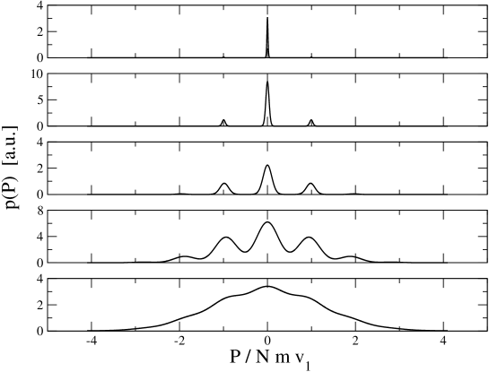
Figure 5: Multi-valley Bogoliubov prediction for the probability distribution $p(P)$ of the total momentum $P$ for an interacting Bose gas of $1000$ particles. Rotation velocity $v_{\rm rot}=0$. Chemical potential $\rho g/k_{B}T_{v}=3.2$. Temperature: $T/T_{v}=0.25,0.5,1,2,3$ (from top to bottom).

The probability distribution $p(P)$ is plotted in fig.5 for $v_{\rm rot}=0$ and different values of the temperature. At low temperatures $T\ll T_{v}$, only a single valley is populated and $p(P)$ shows a single narrow peak around $P=0$. In this case, the gas is nearly fully superfluid. For temperatures growing across $T/T_{v}\approx 1$, higher valleys start to be populated as well, more peaks become visible and the width of each of them gets larger. Correspondingly, the superfluid fraction decreases to zero. At sufficiently high temperature, the isolated peaks merge into a broad, unstructured, distribution. Note that for all temperatures in the figure, the single-valley normal fraction $f_{n}^{v,0}$ remains always significantly smaller than unity.

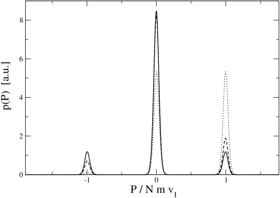
Figure 6: Multi-valley Bogoliubov prediction for the probability distribution $p(P)$ of the total momentum $P$ for an interacting Bose gas of $1000$ particles. Rotation velocity $v_{\rm rot}/v_{1}=0$ (solid), $0.125$ (dashed), $0.5$ (dotted). Chemical potential $\rho g/k_{B}T_{v}=3.2$. Temperature $T/T_{v}=0.5$.

Conventional superfluidity occurs only when the width of the envelope becomes of the order of the spacing between peaks, so that only the one whose quasi-condensate velocity $v_{0}$ is closest to the rotation velocity $v_{\rm rot}$ results effectively populated. Otherwise, mass transport occurs in the presence of a finite rotation velocity $v_{\rm rot}$ as a consequence of the redistribution of population between the different valleys more than of the distortion within a given valley. This behaviour can be clearly observed in fig.6, where the effect of a finite $v_{\rm rot}$ on the probability distribution $p(P)$ is shown: although the shape of each single peak is weakly affected, the envelope function suffers a dramatic distortion.

Let us briefly discuss the validity condition of (66). The validity condition of $|v_{\rm rot}-v_{0}|\ll c$ was already discussed in subsection 4.1. What is left is to compare $k_{B}T|\zeta|$ to $c$. The narrowest features in $p(P)$ are found to be the peaks corresponding to single valley normal fractions, of momentum width $(f_{n}^{v,0}Nmk_{B}T)^{1/2}$. As $g(\zeta)$ is the Fourier transform of $p(P)$, this results in a maximal value of $\zeta$ on the order of

$$\zeta_{\rm max}=\frac{1}{(f_{n}^{v,0}Nmk_{B}T)^{1/2}}.$$ (70)

In the regime $k_{B}T\gg\rho g$, $f_{n}^{v,0}$ is given by the $v=0$ limit of (54). We then obtain

$$\frac{k_{B}T\zeta_{\rm max}}{c}\simeq\frac{1}{(L/\xi)^{1/2}}\ll 1$$ (71)

since we assumed $L\gg\xi$. In the regime $k_{B}T\ll\rho g$, we use (53) with $v=0$ to obtain

$$\frac{k_{B}T\zeta_{\rm max}}{c}\simeq\left(\frac{\hbar c}{Lk_{B}T}\right)^{1/2}.$$ (72)

The condition (66) then imposes a lower bound on the temperature,

$$k_{B}T\gg\hbar c/L.$$ (73)

Since $\hbar c/L$ is the energy of the lowest Bogoliubov excitation in a single valley, this condition is equivalent to a non-zero temperature regime in the valley. Note that this condition is automatically satisfied in the multi-valley regime $T\geq T_{v}$ for a weakly interacting Bose gas.

5 Interacting gas II: classical field model

The results of the previous section have been obtained on the grounds of a Bogoliubov theory which assumes that the density fluctuations are weak; this condition requires the temperature to be sufficiently low $T\ll T_{\rm df}$ where $T_{\rm df}$ is given in (35). On the other hand, for temperatures larger than the chemical potential but still lower than the degeneracy temperature

$$k_{B}T_{\rm deg}\gg k_{B}T\gg\rho g,$$ (74)

a classical field model can be applied. In the present section, we shall discuss the predictions of this approach regarding the superfluidity properties of the gas. The actual existence of a temperature range (74) is guaranteed by the weak interaction condition (34). In this regime, as one can see in the diagram in fig.1, the applicability domains of classical field and Bogoliubov theories have a non-vanishing overlap and, in particular, give coincident predictions, as we shall see.

5.1 The model and its solution

We generalize to the rotating case the classical field model of [13, 20, 21]. In this generalization of the model, the complex field $\psi(z)$ has a grand canonical thermal equilibrium distribution $P[\psi]$ proportional to $\exp(-\beta E[\psi])$ where $E[\psi]$ is the Gross-Pitaevskii energy functional:

$$E[\psi]=\int_{0}^{L}dz\,\left[\frac{\hbar^{2}}{2m}|\partial_{z}\psi|^{2}+\frac{g}{2}|\psi|^{4}-\frac{\hbar}{i}v_{\rm rot}\psi^{*}\partial_{z}\psi-\mu|\psi|^{2}\right]$$ (75)

restricting to the configurations of the complex field obeying the boundary condition $\psi(0)=\psi(L)$.

Expectation values of quantum observables are obtained by replacing $\hat{\psi}$ with $\psi$, $\hat{\psi}^{\dagger}$ with $\psi^{*}$ and then averaging over the thermal distribution $P[\psi]$. At this stage, the reader may argue that a classical field thermal distribution is expected to lead to divergences in the observables in the absence of an energy cut-off, reminiscent of the black-body catastrophe of 19th century. A very fortunate consequence of the 1D character of the gas is that the classical field model gives finite predictions for the observables relevant for this paper, like the mean density, the mean momentum of the gas, the probability distribution of the total momentum of the gas, as we shall see. This suppresses the issue of an energy cut-off dependence.

Calculation of expectation values can be performed exactly in the classical field model: the summation over all possible complex paths $z\rightarrow\psi(z)$ can be viewed formally as a Feynman path integral over trajectories of a single quantum particle in 2D, $z$ playing the role of a fictitious time, the real and imaginary parts of $\psi$ corresponding to fictitious coordinates $x$ and $y$. Using in the reverse order the Feynman formulation of quantum mechanics, one can map the functional integral over all paths into a Feynman propagator for a fictitious Hamiltonian of a quantum particle moving in 2D, here in imaginary time. More details are given in [13, 21]. We give here without proof the expression of the fictitious Hamiltonian for a rotating system:

$${\mathcal{H}}_{v_{\rm rot}}=\frac{p_{x}^{2}+p_{y}^{2}}{2M}+i\frac{m{v_{\rm rot}}}{\hbar}L_{z}+\frac{1}{2}\hbar\beta g(x^{2}+y^{2})^{2}-\hbar\beta(\mu+\frac{1}{2}m{v_{\rm rot}}^{2})(x^{2}+y^{2})$$ (76)

where the fictitious mass is

$$M=\frac{\hbar^{3}}{mk_{B}T},$$ (77)

$p_{x},p_{y}$ are the momentum operators of the fictitious particle along $x,y$ and $L_{z}=xp_{y}-yp_{x}$ is the angular momentum operator of the particle along $z$. Note that the fictitious Hamiltonian is not hermitian for ${v_{\rm rot}}\neq 0$, but its anti-hermitian part commutes with its hermitian part, which is indeed rotationally invariant. A numerical diagonalization of the hermitian part of ${\mathcal{H}}$ is therefore very simple, as one has to solve a Schrödinger equation for the radial part of the eigenfunctions only. The corresponding eigenvectors are labeled by two quantum numbers, the angular momentum $l\in\mathbb{Z}$ and the radial quantum number $n\in\mathbb{N}$, and $E_{n,l}$ is the corresponding real eigenvalue.

5.2 Exact expressions for relevant observables

We give the explicit expression for some useful expectation values. The calculation of the mean density in the classical field model is required to determine the chemical potential $\mu$ for a given mean total number of particles. The mean density is given by

$$\langle\psi^{*}\psi\rangle=\langle x^{2}+y^{2}\rangle_{q}$$ (78)

where the “quantum expectation value” of any operator $O$ for the fictitious particle is defined as

$$\langle O\rangle_{q}\equiv\frac{\mbox{Tr}\left[O\,e^{-L{\mathcal{H}}_{v_{\rm rot}}/\hbar}\right]}{\mbox{Tr}\left[e^{-L{\mathcal{H}}_{v_{\rm rot}}/\hbar}\right]}.$$ (79)

The characteristic function for the total momentum $P=-i\hbar\int\psi^{*}\partial_{z}\psi$ is

$$g(\zeta)=\langle e^{i\zeta P}\rangle=\frac{\mbox{Tr}\left[e^{-L{\mathcal{H}}_{w}/\hbar}\right]}{\mbox{Tr}\left[e^{-L{\mathcal{H}}_{{v_{\rm rot}}}/\hbar}\right]}$$ (80)

where we have introduced the complex velocity

$$w={v_{\rm rot}}-i\zeta k_{B}T$$ (81)

and ${\mathcal{H}}_{w}$ is obtained by replacing $v_{\rm rot}$ with $w$ in ${\mathcal{H}}_{v_{\rm rot}}$. The mean total momentum of the gas is related to the derivative of the characteristic function in $\zeta=0$:

$$\langle P\rangle=-i\frac{dg}{d\zeta}(0)=Nm{v_{\rm rot}}-i\frac{mk_{B}T}{\hbar^{2}}L\langle L_{z}\rangle_{q}$$ (82)

where we used (78) to obtain the mean total number of particles $N$. The first order expansion in $v_{\rm rot}$ of this expression, when combined with the $v_{\rm rot}\rightarrow 0$ limit of (4), leads to the exact expression for the standard definition of the normal fraction [22]:

$$f_{n}^{0}=1-\frac{mk_{B}TL}{\rho\hbar^{2}}\frac{\langle L_{z}^{2}\rangle_{q}(v_{\rm rot}=0)}{\hbar^{2}}.$$ (83)

Note that this expression makes explicit the fact that one has always $f_{n}^{0}\leq 1$, which justifies the name of normal ‘fraction’.

In formula (83) the presence of a non-zero superfluid fraction is related to a non-vanishing expectation value $\langle L_{z}^{2}\rangle_{q}$. This allows to conclude generally that the superfluid fraction tends to zero in the thermodynamical limit: as $L\rightarrow+\infty$, $\exp(-L{\mathcal{H}}_{v_{\rm rot}}/\hbar)$ becomes proportional to the projector on the ground state of the Hermitian part of the fictitious Hamiltonian. As this ground state has a vanishing angular momentum ($l=0$), $\langle L_{z}^{2}\rangle_{q}$ tends to zero in the thermodynamical limit. For a non-zero $v_{\rm rot}$, one gets similarly that $\langle P\rangle/(Nmv_{\rm rot})\rightarrow 1$ in the thermodynamic limit. One sees that the corresponding critical length scale is $L\sim\hbar/\delta E$, where $\delta E$ is the energy difference between the first excited state and the ground state of the hermitian part of ${\mathcal{H}}$. As the minimal energy within a given subspace of angular moment is an increasing function of $|l|$, $\delta E$ is either $E_{n=1,l=0}-E_{n=0,l=0}$ or $E_{n=0,l=1}-E_{n=0,l=0}$. The lengths corresponding to these two possibilities have been identified in [13], they are respectively the correlation length and the coherence length of the bulk. As discussed in [13], the coherence length is actually always larger than the correlation length. One then sees very generally that superfluidity in the spirit of (4) is exponentially suppressed when the length of the sample greatly exceeds the bulk coherence length.

The Bogoliubov approach in previous sections of this paper has produced a physical picture in which a superfluid behavior can still be identified with valleys even when the standard definition (4) gives a normal fraction close to unity. Within the classical field model we can test this prediction in an exact manner, without relying on the Bogoliubov approximation. It is useful first to identify the dimensionless parameters on which the classical field model actually depends. Let us express the field $\psi$ in units of $\rho^{1/2}$ (where $\rho=N/L$ is the mean density) and the spatial coordinate $z$ in units of

$$L_{0}=\frac{\rho\hbar^{2}}{mk_{B}T}.$$ (84)

Note that $L_{0}$ is on the order of the coherence length of the bulk gas, whatever the value of $\chi$ is [13]. One then realizes that $\beta E[\psi]$, and therefore the state of the gas, depends only on (i) $\tilde{v}_{\rm rot}$, the velocity ${v_{\rm rot}}$ in units of $k_{B}T/(\rho\hbar)$, (ii) $\tilde{L}$, the length $L$ in units of $L_{0}$, and (iii) on a dimensionless parameter $\chi$ controlling the interaction strength:

$$\tilde{v}_{\rm rot}\equiv\frac{\rho\hbar v_{\rm rot}}{k_{B}T}\ \ \ \ \tilde{L}\equiv\frac{L}{L_{0}}=2\pi^{2}\frac{T}{T_{v}}\ \ \ \ \chi\equiv\rho L_{0}\frac{\rho g}{k_{B}T}=\left(\frac{L_{0}}{\xi}\right)^{2}=\left(\frac{T_{\rm df}}{T}\right)^{2}$$ (85)

where $\xi$ is the healing length such that $\hbar^{2}/m\xi^{2}\equiv\rho g$, $T_{\rm df}$ is the temperature upper bound (35) required to have weak density fluctuations and $T_{v}$ was defined in (62) in the Bogoliubov approach as the temperature lower bound to have several valleys populated.

For a non-rotating gas, $v_{\rm rot}=0$, we explore the plane of the two remaining parameters, $\tilde{L}$ and $\chi$, by a numerical diagonalization of the fictitious Hamiltonians ${\mathcal{H}}_{v_{\rm rot}}$ and ${\mathcal{H}}_{w}$. This gives access to the probability distribution of $P$ without approximation, and allows to see in which parameter range this distribution has several peaks. The result is plotted in figure (7). As expected, presence of a multi-peaked structure requires a length $L$ larger than $L_{0}$, otherwise the gas is in the Bose-condensed regime. It also requires a large enough $\chi$, that is weak enough density fluctuations. The boundary of the multi-peaked domain is studied analytically in the next subsection, using a large $\chi$ expansion.

For a rotating gas, we have also performed numerical diagonalizations of ${\mathcal{H}}_{v_{\rm rot}}$ and ${\mathcal{H}}_{w}$, which requires in the case of ${\mathcal{H}}_{w}$ the diagonalization of a non-Hermitian matrix. We have recovered the phenomenon, obtained within the Bogoliubov approach, that the peaks of a well resolved multi-peaked structure for $p(P)$ are essentially not shifted by the rotation of the vessel, but their amplitudes depend on $v_{\rm rot}$. The mean momentum of the gas in the classical field model is close to the Bogoliubov prediction in its validity domain, that is for weak density fluctuations, see figure (3).

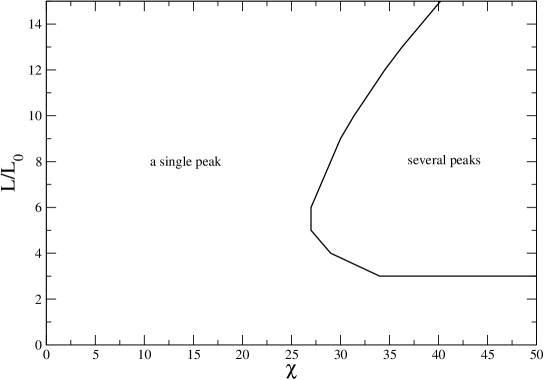
Figure 7: From a full numerical solution of the classical field model, domain in the $\chi-\tilde{L}$ plane where the probability distribution of $p(P)$ is multi-peaked. Only peaks higher than $10^{-3}$ times the maximal value of $p(P)$ were considered, and $\chi$ and $\tilde{L}$ were varied in steps of one.

5.3 Asymptotic expressions

Analytical results can be obtained in two extreme cases. First, in the ideal Bose gas case, where $\chi=0$. The fictitious Hamiltonians appearing in (80) are then quadratic in the position and momentum operators and can be diagonalized exactly. The difference with the usual harmonic oscillator case is that the potential energy term $M\Omega^{2}(x^{2}+y^{2})/2$ is now complex. But one just has to choose for the “oscillation frequency” $\Omega$ the determination of the square root such that $\mbox{Re}\,\Omega>0$ . In this case the usual Gaussian wavefunction $\propto\exp[-m\Omega(x^{2}+y^{2})/2\hbar]$ is a perfectly normalizable “ground state”, and the usual repeated action of the creation operators can be used to obtain the “excited states”. As a consequence the usual 2D isotropic harmonic oscillator spectrum is recovered, ${\mathcal{E}}_{n,l}=(2n+|l|+1)\Omega+imwl$ where $n$ is radial quantum number and $l$ is the angular momentum quantum number. The characteristic function can then be calculated exactly as the sum of a geometrical series:

$$g(\zeta)=\frac{\cosh(\Omega_{v_{\rm rot}}L)-\cos(m{v_{\rm rot}}L/\hbar)}{\cosh(\Omega_{w}L)-\cosh[mL(\zeta k_{B}T-i{v_{\rm rot}})/\hbar]}$$ (86)

where the complex oscillation frequencies are such that

$$\Omega_{w}^{2}=-\frac{2m}{\hbar^{2}}(\mu+\frac{1}{2}mw^{2})\ \ \ \ \mbox{and}\ \ \ \ \Omega_{v_{\rm rot}}^{2}=-\frac{2m}{\hbar^{2}}(\mu+\frac{1}{2}m{v_{\rm rot}}^{2}).$$ (87)

and $w$ was introduced in (81). The resulting $p(P)$ is shown in the appendix A to have a single maximum, at least for $v_{\rm rot}=0$. The chemical potential was already calculated in the classical field approximation, using the Poisson summation formula, see (26). Using (82) one also recovers the expression (27) for the mean momentum. So, for the ideal Bose gas in the classical field model, using the Feynman formula to relate a path integral to the trace of an evolution operator is similar to the use of the Poisson summation formula!

Second, in the large $\chi$ limit, where intensity fluctuations of the field become weak, one can obtain asymptotic formulas for $g(\zeta)$. In this limit, the coherence length $L_{0}$ is much larger than the healing length $\xi$. To simplify the calculation, we take ${v_{\rm rot}}=0$ in a first stage and we restrict to the case of a length $L$ on the order of a few times the coherence length and therefore much larger than $\xi$ [13]: in this case, the energy differences $E_{n=1,l}-E_{n=0,l}$ are much larger than $\hbar/L$ so that, within each subspace of fixed angular momentum $l$, one can restrict to the ground state of the Hermitian part of the fictitious Hamiltonian in the calculation of $g(\zeta)$:

$$g(\zeta)\propto\sum_{l\in\mathbb{Z}}e^{-L(E_{0,l}+ml\zeta k_{B}T)/\hbar}$$ (88)

where the normalization factor is obtained from $g(0)=1$ and $E_{0,l}$ is the lowest eigenenergy of the Hermitian part of ${\mathcal{H}}_{w}$ with angular momentum $l$ (remember that $v_{\rm rot}=0$ here). Using polar coordinates $r,\theta$, we write the corresponding wavefunction $\phi_{0,l}$ as

$$\phi_{0,l}(x,y)=f_{l}(r)\frac{e^{il\theta}}{(2\pi r)^{1/2}}$$ (89)

where $r=(x^{2}+y^{2})^{1/2}/\rho^{1/2}$. The purely radial wavefunction then solves the Schrödinger equation

$$-\frac{1}{2}\frac{d^{2}}{dr^{2}}f_{l}(r)+U_{l}(r)f_{l}(r)=\tilde{E}_{0,l}f_{l}(r)$$ (90)

with an effective potential $U_{l}$ including a centrifugal term:

$$U_{l}(r)=\frac{l^{2}-1/4}{2r^{2}}+\frac{1}{2}\chi r^{4}-(\tilde{\mu}-\tilde{\zeta}^{2}/2)r^{2}$$ (91)

where $\tilde{\zeta}=\rho\hbar\zeta$, $\tilde{E}_{0,l}=L_{0}E_{0,l}/\hbar$, and where the reduced chemical potential $\tilde{\mu}=\rho L_{0}\mu/(k_{B}T)$ is here close to its bulk value calculated for large $\chi$ in [13], since $L$ exceeds a few $L_{0}$:

$$\tilde{\mu}=\chi+\frac{1}{2}\chi^{1/2}+O(1).$$ (92)

In the large $\chi$ limit, the ground state is deeply localized in the minimum of $U_{l}(r)$ occurring at a non-zero distance $r_{l}$ from the origin, solution of $U^{\prime}(r_{l})=0$. One can then expand $U_{l}(r)$ in a power series around $r=r_{l}$, include the quadratic part in $(r-r_{l})^{2}$ in a harmonic oscillator diagonalization, include the cubic, quartic, $\ldots$ terms with perturbation theory. Treatment of up to quartic terms with second order perturbation theory turns out to be sufficient here:

$$\tilde{E}_{0,l}=U_{l}(r_{l})+\frac{1}{2}\omega_{l}+\frac{3U_{l}^{(4)}(r_{l})}{96\omega_{l}^{2}}-\frac{11\left[U_{l}^{(3)}\right]^{2}}{288\omega_{l}^{4}}+\ldots$$ (93)

where $\omega_{l}=[U^{(2)}(r_{l})]^{1/2}$ is the oscillation frequency in the harmonic approximation to $U_{l}(r)$. The position $r_{l}$ can be calculated exactly, since $r_{l}^{2}$ is found to be the root of a cubic equation; when (93) is plugged into (88), one gets a very good approximation for $g(\zeta)$ and, by numerical Fourier transform, a very good approximation for the probability distribution of $P$, as compared to the full numerical solution, for $\chi\gg 1$, see figure 8. A more tractable expression can be obtained by realizing that typical values of $\tilde{\zeta}^{2}$ and $l^{2}$ are of order $\chi^{1/2}$ , and by performing a systematic expansion of the cubic equation for $r_{l}$ and of (93) in powers of ${\chi}^{-1/2}$:

$$\tilde{E}_{0,l}-l\tilde{\zeta}=\mbox{const}+\frac{1}{2}(\tilde{z}-l)^{2}+\frac{l^{2}}{2\chi^{1/2}}-\frac{1}{8\chi}(l^{2}-\tilde{\zeta}^{2})^{2}+O(\chi^{-1/2})$$ (94)

where const depends on $\chi$ only, not on $l$ or $\zeta$. The second term in the righthand side of the equation is $O(\chi^{1/2})$, the third and fourth terms are a priori of the same order $O(1)$. In practice the fourth term is typically $O(\chi^{-1/2})$ so we neglect it . We then obtain a Gaussian expressions for $g(\zeta)$ and $p(P)$.

The previous calculations are immediately generalized to the case of a non-zero velocity: as $L>L_{0}$, $\mu+m{v_{\rm rot}}^{2}/2$ depends weakly on ${v_{\rm rot}}$ and can be replaced by the bulk value for ${v_{\rm rot}}=0$; one then has to replace $\tilde{\zeta}^{2}$ by $\tilde{\zeta}^{2}-2i\tilde{v}_{\rm rot}\tilde{\zeta}$ in the above calculation of $\tilde{E}_{0,l}$, where $\tilde{v}_{\rm rot}$, being independent on $\chi$, is $O(1)$. We then obtain for $g(\zeta)$:

$$g(\zeta)=A\sum_{l\in\mathbb{Z}}e^{-\tilde{L}(l-\tilde{\zeta}+i\tilde{v}_{\rm rot})^{2}/2}e^{-\tilde{L}l^{2}/(2\chi^{1/2})}$$ (95)

where $A$ is a constant factor such that $g(0)=1$. Performing the Fourier transform of this expression and using the Poisson summation formula leads to

$$p(P)=Be^{-(\tilde{P}-\tilde{L}\tilde{v}_{\rm rot})^{2}/(2\tilde{L})}\sum_{q\in{\mathbb{Z}}}e^{-(\tilde{P}-2\pi q)^{2}\chi^{1/2}/(2\tilde{L})}$$ (96)

where $\tilde{P}=P/(\rho\hbar)$. The constant factor $B$ is such that the integral of $p(P)$ over $P$ is equal to unity. Formula (96) is very suggestive, as it is simply a Gaussian envelope centered in $\tilde{P}=\tilde{L}\tilde{v}_{\rm rot}$ on top of a periodic train of Gaussian peaks separated by $2\pi$ in $\tilde{P}$ space. Therefore the function $p(P)$ is multi-peaked if the envelope has a width larger than $2\pi$ and if each Gaussian of the train has a width less than $2\pi$:

$$\tilde{L}^{1/2}>2\pi\ \ \ \mbox{and}\ \ \ (\chi^{1/2}/\tilde{L})^{1/2}>2\pi.$$ (97)

One recovers the conditions (69) using the fact that $f_{n}^{0}=\chi^{-1/2}$ in the classical field regime $k_{B}T>\rho g$, see (54).

The asymptotically exact expression (96) is successfully compared with the full numerical solution in figure 8. One can also compare it to the Bogoliubov prediction (68): the two predictions are found to be identical up to higher order terms (see appendix C). As a consequence, all the physical discussion following (68) also holds for the classical field model! From (95) one can also calculate the normal fraction $f_{n}^{0}$ for ${v_{\rm rot}}=0$ by taking the second order derivative of (95) with respect to $\zeta$. Equivalently one may calculate the variance of $P$ from (96) and use (13). One gets two equivalent forms:

$$f_{n}^{0}=1-\frac{L}{L_{0}}\frac{\sum_{q}q^{2}\exp(-\tilde{L}_{\rm eff}q^{2}/2)}{\sum_{q}\exp(-\tilde{L}_{\rm eff}q^{2}/2)}=\frac{1}{{\chi}^{1/2}+1}+\frac{1}{L(1+\chi^{-1/2})^{2}}\frac{\sum_{q\in{\mathbb{Z}}}(2\pi q)^{2}e^{-(2\pi q)^{2}/(2\tilde{L}_{\rm eff})}}{\sum_{q\in{\mathbb{Z}}}e^{-(2\pi q)^{2}/(2\tilde{L}_{\rm eff})}}$$ (98)

where the reduced effective length is $\tilde{L}_{\rm eff}=L(1+\chi^{-1/2})/L_{0}$. The first form immediately shows that $f_{n}^{0}$ tends to one exponentially for $L\gg L_{0}$. The second form recovers the formula (11) of [5] in a calculation up to first order in ${\chi}^{-1/2}$ where one replaces $\rho_{S}$ of [5] by $\rho(1-{\chi}^{-1/2})$.

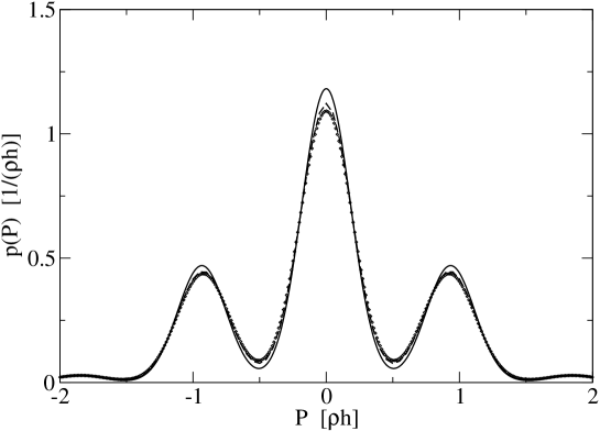
Figure 8: Probability distribution of the total momentum $P$ in the classical field model, for $\chi=200$, $v_{\rm rot}=0$ and $L/L_{0}=20$. Symbols: full numerical solution. Solid line: analytical expression (96). Dashed line: semi-analytical prediction resulting from the use of $r_{l}$ as given by the exact solution of $U^{\prime}(r_{l})=0$ (see text). The dashed line and the symbols are almost indistinguishable.

6 Conclusions

We have investigated the superfluid properties of a ring of degenerate and weakly interacting 1D Bose gas at thermal equilibrium with a rotating vessel at velocity $v_{\rm rot}$. Provided the transverse trapping is strong enough, our model is a good description of a Bose gas confined in a toroidal trap [11].

Using the conventional definition of the superfluid fraction, which relies on the variance of the total momentum of the gas in the limit $v_{\rm rot}\rightarrow 0$, we find that the gas has a significant superfluid fraction only in the Bose condensed regime, that is when the length of the ring does not exceed the coherence length of the bulk gas $l_{c}\sim\rho\lambda^{2}$, $\rho$ being the mean density and $\lambda$ the thermal de Broglie wavelength.

To investigate more carefully the regime where the length of the ring exceeds the coherence length, we have considered the full probability distribution of the total momentum $P$. We have identified a regime where several peaks appear in this probability distribution, each peak corresponding to a quasicondensate in a plane wave state with a given winding number, the analog of supercurrents in superconductors. Each supercurrent state exhibits some superfluid behaviour: in presence of a non-zero $v_{\rm rot}$, the peaks in the probability distribution of $P$ are indeed not shifted. This allows to define a local normal fraction for an individual supercurrent. Quantitatively, we have found that the probability distribution of $P$ shows several isolated peaks provided that the length of the ring in units of the coherence length does not exceed the inverse of the local normal fraction.

In this non-Bose-condensed regime, it is obvious that the conventional criterion for superfluidity based on the variance of $P$ is sensitive to the envelope of the distribution but does not catch its multi-peaked structure. To get it, a direct measurement of the total current $P$ is required, which, e.g., could be performed by means of the technique proposed in [23]: in a slow-light regime, the dielectric susceptibility of the atoms depends on the local value of the matter current so that the phase accumulated by light after a round-trip around the ring is proportional to the total current $P$.

Appendix A Absence of multiple peaks in $p(P)$ for the ideal gas

The characteristic function for the ideal gas in the classical field regime is:

$$g(\zeta)=\prod_{k}\frac{\beta(\epsilon_{k}-\mu)}{\beta(\epsilon_{k}-\mu)-i\zeta\hbar k}.$$ (99)

In the $v_{\rm rot}=0$ case, we can regroup the pairs $\pm k$ and rewrite (99) as:

$$g(\zeta)=\prod_{k>0}g_{k}(\zeta)=\prod_{k>0}\frac{\beta^{2}(\epsilon_{k}-\mu)^{2}}{\beta^{2}(\epsilon_{k}-\mu)^{2}+(\hbar k)^{2}\,\zeta^{2}}.$$ (100)

The Fourier transform $p_{k}(P)$ of each term $g_{k}(\zeta)$ is then:

$$p_{k}(P)=\frac{\eta_{k}}{2}e^{-\eta_{k}\,|P|},$$ (101)

with $\eta_{k}=\beta(\epsilon_{k}-\mu)/\hbar k$. In particular, $p_{k}(P)$ has the property of being an even function that is decreasing for $P>0$ (let’s call this property ${\mathcal{P}}$). As the characteristic function $g(\zeta)$ is the product of the $g_{k}(\zeta)$, the distribution function $p(P)$ is the convolution of the $p_{k}(P)$. As the convolution of two functions with the property ${\mathcal{P}}$ gives again a function with the property ${\mathcal{P}}$ (a sketch of the proof is given below), we can conclude that the probability distribution $p(P)$ for the ideal gas has a single maximum, which is at $P=0$. The possibility of multi-peaked structures is therefore ruled out for the ideal gas in the classical field regime.

We can prove that the property ${\mathcal{P}}$ is preserved by convolution operations in the following way. Let $p_{1}(P)$ and $p_{2}(P)$ be two arbitrary functions sharing property ${\mathcal{P}}$. We have to prove that:

$$p_{c}(P)=\int\!dP^{\prime}\,p_{1}(P^{\prime})\,p_{2}(P-P^{\prime})$$ (102)

• is an even function.

• is a monotonically decreasing function for $P>0$. Let’s compute its derivative for $P>0$:

  $$p_{c}^{\prime}(P)=\int\!dP^{\prime}\,p_{1}(P^{\prime})\,p_{2}^{\prime}(P-P^{\prime})=\int\!dP^{\prime}\,p_{1}(P-P^{\prime})\,p_{2}^{\prime}(P^{\prime})=\\ =\int_{0}^{\infty}\!dP^{\prime}\,p_{2}^{\prime}(P^{\prime})\Big{[}p_{1}(P-P^{\prime})-p_{1}(P+P^{\prime})\Big{]}.$$ (103)

  As $|P-P^{\prime}|<|P+P^{\prime}|$ and $p_{1}$ is a decreasing function of the absolute value of its argument, the integrand is negative. This guarantees that $p_{c}^{\prime}(P)<0$ for all $P>0$.

Appendix B Derivation of the Bogoliubov Hamiltonian and momentum operator

The Hamiltonian (42) can be obtained either by directly solving the Bogoliubov-de Gennes equations for a moving system, or, better, by applying Galilean invariance arguments to the well-known case of a system at rest. The eigenstates of a weakly interacting Bose gas at rest ($v_{0}=0$) are labeled within Bogoliubov theory by the occupation number of the bosonic quasiparticle modes $\{n_{k}\}$. Thanks to translational invariance, these eigenstates are also eigenstates of the momentum: each quasiparticle carrying a momentum $\hbar k$, the total momentum of the gas is given by:

$$P[\{n_{k}\}]=\sum_{k\neq 0}\hbar k\,n_{k}.$$ (104)

Omitting for the moment the rotation energy $-Pv_{\rm rot}$, the total energy is given by:

$$E_{v_{\rm rot}=0}[\{n_{k}\}]=E_{GP}[v_{\rm rot}=0,v_{0}=0]-\sum_{k\neq 0}\epsilon^{0}_{k}\,V_{k}^{2}+\sum_{k\neq 0}\epsilon^{0}_{k}\,n_{k}.$$ (105)

The properties of a moving quasi-condensate at $v_{0}\neq 0$ can be obtained from the ones of a quasi-condensate at rest by transforming the energy and the momentum via a Galilean transformation of velocity $v=v_{0}$. As discussed in sec.2.1, the total momentum $P^{\prime}$ in the moving frame is in fact given by:

$$P^{\prime}[\{n_{k}\}]=P[\{n_{k}\}]+Nmv_{0}=\sum_{k\neq 0}\hbar k\,n_{k}+Nmv_{0}.$$ (106)

Inserting back the rotation term $-P^{\prime}v_{\rm rot}$, the energy $E^{\prime}$ turns out to be:

$$E^{\prime}[\{n_{k}\}]=E_{v_{\rm rot}=0}[\{n_{k}\}]+\frac{1}{2}Nmv_{0}^{2}+(v_{0}-v_{\rm rot})P[\{n_{k}\}]=\\ =E_{GP}[v_{\rm rot},v_{0}]-\sum_{k\neq 0}\epsilon^{0}_{k}\,V_{k}^{2}+\sum_{k\neq 0}\big{[}\epsilon^{0}_{k}+\hbar k(v_{0}-v_{\rm rot})\big{]}\,n_{k}.$$ (107)

The eigenstates and eigenenergies obtained in this way exactly correspond to the ones of the Bogoliubov Hamiltonian (42). For each state, the total momentum (106) agrees with (46).

Appendix C Comparison of Bogoliubov and classical field theory for $p(P)$

In the regime of weak density fluctuations and a temperature $k_{B}T\gg\rho g$ we compare the expressions for the total momentum probability distribution $p(P)$ obtained by Bogoliubov theory, (68) on one side, and by a large $\chi$ expansion of the classical field model, (96) on the other side. At first glance, (96) looks much simpler and therefore different than (68). However one has the identity

$$\tilde{L}^{-1}(\tilde{P}-\tilde{L}\tilde{v}_{\rm rot})^{2}+\tilde{L}^{-1}(\tilde{P}-2\pi q)^{2}\chi^{1/2}=\tilde{L}^{-1}(1+\chi^{1/2})\left(\tilde{P}-\tilde{P_{0}}\right)^{2}+\tilde{L}^{-1}\frac{(2\pi q-\tilde{L}\tilde{v}_{\rm rot})^{2}}{1+\chi^{-1/2}}$$ (108)

where

$$\tilde{P}_{0}=\frac{\tilde{L}\tilde{v}_{\rm rot}+2\pi q{\chi}^{1/2}}{{\chi}^{1/2}+1}.$$ (109)

Expanding ${\tilde{P}}_{0}$ up to first order in ${\chi}^{1/2}$ and using the fact that $f_{n}^{v,0}={\chi}^{-1/2}$ in the Bogoliubov theory, one finds that $\tilde{P}-\tilde{P_{0}}$ coincides with the expression in square brackets in (68). The factor in front of this expression, proportional to $1/f_{n}^{v,0}$, recovers ${\tilde{L}}^{-1}(1+\chi^{1/2})$ within leading order in ${\chi}^{1/2}$. The last term in (108) coincides with the argument of the first exponential factor in (68) when expanded up to first order in ${\chi}^{-1/2}$.

References

- [1] K. Huang. Statistical Mechanics, Wiley (New York, 1987).
- [2] V. N. Popov, Functional Integrals in Quantum Field Theory and Statistical Physics, D. Reidel publishing company (Dordrecht, Holland, 1983), chapter 6 and references therein.
- [3] E. B. Sonin, JETP 32, 773 (1971).
- [4] A. J. Leggett, Rev. Mod. Phys. 71, S318 (1999).
- [5] N. V. Prokof’ev and B. V. Svistunov, Phys. Rev. B 61, 11282 (2000)
- [6] K. W. Madison, F. Chevy, W. Wohlleben, and J. Dalibard, Phys. Rev. Lett. 84, 806 (2000).
- [7] J.R. Abo-Shaeer, C. Raman, J.M. Vogels, and W. Ketterle, Science 292, 476 (2001).
- [8] P. C. Haljan, I. Coddington, P. Engels, and E. A. Cornell, Phys. Rev. Lett. 87, 210403 (2001)
- [9] E. Hodby, G. Hechenblaikner, S. A. Hopkins, O. M. Maragò, and C. J. Foot, Phys. Rev. Lett. 88, 010405 (2002)
- [10] E. H. Lieb and W. Liniger, Phys. Rev. 130, 1605 (1963).
- [11] E. J. Mueller, P. M. Goldbart, and Y. Lyanda-Geller Phys. Rev. A 57, R1505 (1998); Ph. Verkerk and D. Hennequin, preprint physics/0306155.
- [12] C. Cohen-Tannoudji, lecture notes at Collège de France, academic year 2001-2, available at the website: http://www.phys.ens.fr/cours/college-de-france/2001-02/2001-02.htm.
- [13] Y. Castin, R. Dum, E. Mandonnet, A. Minguzzi, I. Carusotto, J. Mod. Opt. 47, 2671 (2000).
- [14] P.E. Sokol, “Bose-Einstein Condensation in Liquid Helium”, in Bose-Einstein Condensation, edited by A. Griffin, D.W. Snoke, and S. Stringari, Cambridge University Press (New York, 1995).
- [15] P. Nozières and D. Pines, in The Theory of Quantum Liquids, vol. 1 and vol. 2, (Redwood City: Addison-Wesley, 1990)
- [16] C. Mora and Y. Castin, Phys. Rev. A 67, 053615 (2003)
- [17] For a review of the Bogoliubov approach, see Y. Castin, in ’Coherent atomic matter waves’, Lecture Notes of Les Houches Summer School, p.1-136, edited by R. Kaiser, C. Westbrook, and F. David, EDP Sciences and Springer-Verlag (2001), and references therein.
- [18] I. Carusotto, Y. Castin, and J. Dalibard, Phys. Rev. A 63, 023606 (2001); I. Carusotto and Y. Castin, J. Phys. B 34, 4589 (2001).
- [19] I. Carusotto and Y. Castin, Phys. Rev. Lett. 90, 030401 (2003).
- [20] D. J. Scalapino, M. Sears, and R. A. Ferrell, Phys. Rev. B 6, 3409 (1972).
- [21] Y. Castin, Lecture notes in Les Houches summer school on quantum gases with reduced dimensionality, April 2003, edited by H. Perrin, L. Pricoupenko, M. Olshanii, to be published.
- [22] We used the fact that the chemical potential varies only to second order in when the mean density is fixed.
- [23] M. Artoni and I. Carusotto, Phys. Rev. A 67, 011602 (2003).