Test-charge theory for the electric double layer

Abstract

We present a model for the ion distribution near a charged surface, based on the response of the ions to the presence of a single test particle. Near an infinite planar surface this model produces the exact density profile in the limits of weak and strong coupling, which correspond to zero and infinite values of the dimensionless coupling parameter. At intermediate values of the coupling parameter our approach leads to approximate density profiles that agree qualitatively with Monte-Carlo simulation. For large values of the coupling parameter our model predicts a crossover from exponential to algebraic decay at large distance from the charged plate. Based on the test charge approach we argue that the exact density profile is described, in this regime, by a modified mean field equation, which takes into account the interaction of an ion with the ions close to the charged plate.

I Introduction

Interactions between charged objects in solution are determined by the distribution of ions around them. Understanding these distributions is thus of fundamental importance for theoretical treatment of water soluble macromolecules such as polyelectrolytes, charged membranes, and colloids LesHouches ; PhysicsToday . In recent years, much interest has been devoted to correlation effects in ionic solutions and to attempts to go beyond mean field theory in their treatment. In particular it has been realized that such effects can lead to attractive interactions between similarly charged objects, as was demonstrated in theoretical models KAJM92 ; StevensRobbins90 ; NetzOrland99 ; LukatskySafran99 ; Shklovskii ; HaLiu97 ; PodZeks88 ; Netz01 , simulation GJWL84 ; KAJM92 ; DAH03 ; GMBG97 ; MoreiraNetz02 and experiment KMQ88 ; KMSS93 ; Bloomfield91 ; Raspaud98 ; RauParsegian .

Despite the theoretical interest in ion correlation effects, they are not fully understood even in the most simple model for a charged object surrounded by its counterions, shown schematically in Fig. 1. The charged object in this model is an infinite planar surface localized at the plane $z=0$, having a uniform charge density $\sigma$. The charged plate is immersed in a solution of dielectric contact $\varepsilon$ and is neutralized by a single species of mobile counterions (there is no salt in the solution). These counterions are confined to the half space $z>0$ and each one of them carries a charge $e$, which is a multiple of the unit charge for multivalent ions. The ions are considered as point-like, i.e., the only interactions in the system, apart from the excluded volume at $z<0$, are electrostatic.

The system described above is characterized by a single dimensionless coupling parameter NetzOrland00

$$\Xi=\frac{2\pi e^{3}\sigma}{(\varepsilon k_{B}T)^{2}}$$ (1)

where $k_{B}T$ is the thermal energy. At small values of this coupling parameter the electrostatic interaction between ions is weak. As a result, in the limit $\Xi\rightarrow 0$ mean field theory is exact, as can be formally proved using a field-theory formulation of the problem NetzOrland00 . Correlations between ions close to the charged plate play a progressively more important role with increase of the coupling parameter. From Eq. (1) one sees that this happens with an increase of the surface charge, with decrease of the temperature or dielectric constant, and with increase of the charge or, equivalently, the valency of counterions. The model of Fig. 1 thus provides an elementary theoretical framework for studying ion correlation effects near charged objects, with no free parameters other than $\Xi$, which tunes and controls the importance of ion correlations.

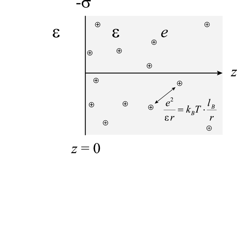
Figure 1: Schematic description of the double layer model considered in this work. An infinite charged plate having a uniform surface charged density $\sigma$ is immersed in a dielectric medium having dielectric constant $\varepsilon$ on both sides of the plate. The charge of the plate is neutralized by point-like counterions, carrying each a charge $e$. These ions are confined to the positive $z$ half space, where $z=0$ is the plane occupied by the plate. In thermal ($k_{B}T$) units the interaction between two ions is given by $l_{B}/r$, where $r$ is the distance between the ions and $l_{B}=e^{2}/(\varepsilon k_{B}T)$ is the Bjerrum length.

In recent years two theoretical approaches were proposed for treatment of the strong coupling limit $\Xi\rightarrow\infty$. The first approach Shklovskii is based on properties of the strongly coupled, two dimensional one component plasma, and emphasizes the possibility of Wigner crystal like ordering parallel to the charged plane. The second approach Netz01 is formally an exact, virial type expansion applied to a field-theory formulation of the partition function. Both of these approaches predict an exponential decay of the ion density distribution in the strong coupling limit, leading to a more compact counterion layer than in mean field theory.

Although the form of the density profile is established in the two limits $\Xi\rightarrow 0$ and $\Xi\rightarrow\infty$, its behavior at intermediate values of the coupling parameter is still not clear. Liquid-state theory approaches such as the AHNC approximation KjelMar can probably be used in this regime, but in practice they were applied in the literature only to relatively small values of the coupling parameter, usually also including ingredients other than those in the model of Fig. 1 – such as finite ion size, added salt, or an interaction between two charged planar surfaces. The infinite planar double layer with no added salt (Fig. 1) was recently studied using Monte-Carlo computer simulation MoreiraNetz02 , providing detailed results on the counterion distribution in a wide range of coupling parameter values. These results validate the expected behavior in the weak and strong coupling limits. In addition they provide new data at intermediate values of the coupling parameter, to which theoretical approaches can be compared.

We propose, in the present work, a new theoretical approach for treating the distribution of counterions near the charged plate. This approach is based on an approximate evaluation of the response of the ionic layer, to the presence of a single test particle. While an exact evaluation of this response would, in principle, allow the distribution of ions to be obtained exactly, we show that even its approximate calculation provides meaningful and useful results. In the limits of small and large $\Xi$ the exact density profile is recovered. At intermediate values of the coupling parameter our approach agrees semi-quantitatively with all the currently available simulation data.

The outline of this work is as follows. In Sec. II we present the model and discuss why it produces the exact density profile in the weak and strong coupling limits. In Sec. III we present numerical results for the density profile close to the charged plate, and compare them with simulation results of Ref. MoreiraNetz02 . Numerical results of our model, further away from the charged plate, where there is currently no data from simulation, are presented in Sec. IV, and scaling results are obtained for the behavior of our model in this regime. Finally, in Sec. V we discuss the relevance of our model’s predictions, at small and large $z$, to the exact theory. Many of the technical details and derivations appear in the appendices at the end of this work.

II Model

II.1 Scaling

Consider the system shown in Fig. 1, with the parameters $\sigma$, $e$, $\varepsilon$ defined in the introduction. We will first express the free energy using the dimensionless coupling parameter $\Xi$. In the canonical ensemble the partition function can be written as follows ($z_{i}$ is the $z$ coordinate of the $i$-th ion):

$${\rm exp}(-F_{N})=\frac{1}{N!}\int\prod_{i=1}^{N}{\rm d}^{3}{\bf r}_{i}\,{\rm exp}\left[-\sum_{i=1}^{N}\frac{z_{i}}{\mu}-\sum_{j>i}\frac{l_{B}}{\left|{\bf r}_{i}-{\bf r}_{j}\right|}\right]$$ (2)

where $l_{B}=e^{2}/\varepsilon k_{B}T$ is the distance at which the Coulomb energy of two ions is equal to the thermal energy $k_{B}T$, and $\mu=e/(2\pi l_{B}\sigma)$ characterizes the bare interaction of an ion with the charged plane. These quantities, the only two independent length scales in the problem, are known as the Bjerrum length and Gouy-Chapman length, respectively. We rescale the coordinates by the Gouy-Chapman length:

$$\tilde{\bf r}_{i}=\frac{{\bf r}_{i}}{\mu},$$ (3)

yielding ${\rm exp}(-F_{N})=(\mu)^{3N}{\rm exp}(-\tilde{F_{N}})$, where

$${\rm exp}(-\tilde{F_{N}})=\frac{1}{N!}\int\prod_{i=1}^{N}{\rm d}^{3}\tilde{\bf r}_{i}\,{\rm exp}\left[-\sum_{i=1}^{N}\tilde{z}_{i}-\sum_{j>i}\frac{\Xi}{\left|\tilde{\bf r}_{i}-\tilde{\bf r}_{j}\right|}\right]$$ (4)

and the ratio

$$\Xi=\frac{l_{B}}{\mu}$$ (5)

is the coupling parameter that was previously defined in Eq. (1). The requirement of charge neutrality is: $N/A=\sigma/e$, where $A$ is the planar area. Hence the number of ions per rescaled unit area is equal to:

$$\frac{N}{\tilde{A}}=\frac{1}{2\pi\Xi}$$ (6)

where $\tilde{A}=A/\mu^{2}$. The local density of ions in the rescaled coordinates is equal to $\tilde{\rho}({\bf r})=\mu^{3}\tilde{\rho}({\bf r})$. Due to symmetry this density depends only on $\tilde{z}$ and it is convenient to define a normalized, dimensionless, density per unit length:

$$\tilde{n}(\tilde{z})=2\pi l_{B}\mu^{2}\rho=2\pi\Xi\tilde{\rho}$$ (7)

having the property:

$$\int_{0}^{\infty}{\rm d}\tilde{z}\,\tilde{n}(\tilde{z})=1$$ (8)

as seen from Eqs. (6) and (7). From here on we will omit the tilde symbol ($\sim$) from all quantities, in order to simplify the notations. In order to express physical quantities in the original, non-scaled units, the following substitutions can be used:

$${\bf r} \rightarrow {\bf r}/\mu$$ (9)

$$n \rightarrow 2\pi l_{B}\mu^{2}\rho$$ (10)

We will also omit the subscript $N$ from the free energy $\tilde{F}_{N}$, implying that $N$ is determined by charge neutrality.

II.2 Known results in the limits of small and large $\Xi$

We briefly review some known properties of the ion distribution in the limits of small and large $\Xi$ (for a more complete discussion, see Ref. Netz01 ). In the limit of $\Xi\rightarrow 0$ mean field theory becomes exact. The density profile is obtained from the Poisson-Boltzmann (PB) equation and decays algebraically, having the form AndelmanReview

$$n_{\rm PB}(z)=\frac{1}{(z+1)^{2}}$$ (11)

Within the adsorbed layer ions form a three dimensional, weakly correlated gas: the electrostatic interaction between neighboring ions is small compared to the thermal energy. This last statement can be verified by considering the density of ions at contact with the plane, $\rho_{\rm PB}(0)=1/(2\pi\Xi)$ (see Eqs. (7) and (11)). The typical distance between neighboring ions is thus of order $\Xi^{1/3}$. In the non-scaled units this distance is much larger than $l_{B}$, which validates the statement that ions are weakly correlated: $\Xi^{1/3}\mu=\Xi^{-2/3}l_{B}\gg l_{B}$. Note also that this typical distance is small compared to the width of the adsorbed layer (Gouy-Chapman length): $\Xi^{1/3}\mu\ll\mu$.

In the opposite, strong coupling (SC) limit of $\Xi\gg 1$, the density profile decays exponentially,

$$n_{\rm SC}(z)={\rm exp}(-z)$$ (12)

The width of the adsorbed layer is still of order $\mu$ in the non-scaled units, but is now small compared to $l_{B}$. Equation (6) indicates that the average lateral distance between ions is then of order $\Xi^{1/2}$. This distance is large compared to the width of the ionic layer, $\Xi^{1/2}\mu\gg\mu$. On the other hand it is small in units of the Bjerrum length: $\Xi^{1/2}\mu=\Xi^{-1/2}l_{B}\ll l_{B}$. The ions form, roughly speaking, a two-dimensional sheet and are highly correlated within this adsorbed layer. The typical lateral separation between ions, $\Xi^{1/2}$, is an important length scale in the strong coupling limit, and will play an important role also in our approximated model.

At sufficiently large values of $\Xi$ it has been conjectured (but not proved) that ions form a two-dimensional, triangular close-packed Wigner crystal parallel to the charged plate. Based on the melting temperature of a two dimensional, one component plasma, one can estimate that this transition occurs at $\Xi\gtrsim 31,000$ Shklovskii ; MoreiraNetz02 . Furthermore, the ion-ion correlation function is expected to display short range order similar to that of the Wigner crystal even far below this transition threshold. The exponential decay of Eq. (12) was predicted, based on these notions, in Ref. Shklovskii . The same result can be obtained also in a formal virial expansion Netz01 , which is valid for large $\Xi$ but does not involve long range order parallel to the charged plate at any value of $\Xi$.

Finally we note two general properties of the density profile that are valid at any value of $\Xi$. First, the normalized contact density $n(0)$ is always equal to unity – a consequence of the contact theorem CarnieChan81 (see also Appendix D). Second, the characteristic width of the adsorbed layer is always of order unity in the rescaled units. These two properties restrict the form of the density distribution quite severely and indeed the two profiles (11) and (12) are similar to each other close to the charged plane. Far away from the plate, however, they are very different from each other: at $z\gg 1$ the probability to find an ion is exponentially small in the SC limit, while in the weak coupling limit it decays only algebraically and is thus much larger. Furthermore, in the weak coupling case, moments of the density, including the average distance of an ion from the plate, diverge.

Although the form of the density profile is known in the limits of small and large $\Xi$, two important issues remain open. The first issue is the form of the density profile at intermediate values of $\Xi$. At coupling parameter values such as 10 or 100 perturbative expansions around the limits of small or large $\Xi$ NetzOrland00 ; Netz01 are of little use, because they tend to give meaningful results only at small values of their expansion parameter. Such intermediate values are common in experimental systems with multivalent ions, as demonstrated in Table 1. Second, even at very small or very large $\Xi$ the respective asymptotic form of $n(z)$ may be valid within a limited range of $z$ values. In particular, for large $\Xi$ it is natural to suppose that sufficiently far away from the charged plate the density profile crosses over from SC to PB behavior. Indeed, far away from the plate the ion density is small, resembling the situation near a weakly charged surface. The main objective of this work is to investigate these issues, both of which necessitate going beyond the formal limits of vanishing and infinite $\Xi$.

Table 1: Characteristic values of $\sigma$, $\mu$ and $\Xi$ for several representative macromolecules. Values of $\Xi$ are shown for two cases: monovalent counterions (1-$e$) and $4$-valent ones (4-$e$). The Gouy-Chapman length $\mu$ corresponds to monovalent ions. The cell membrane charge density is estimated assuming that 10 % of the lipids in the membrane are charged. The surface charge of DNA is estimated from the linear charge density along the DNA contour, equal to $1/1.7$ $e$/Å, and assuming a radius of 10 Å. For Mica full dissociation of charged groups is assumed. In all three cases the Bjerrum length is taken as $l_{B}=7$ Å, which corresponds to water at room temperature.

	$\sigma$($e$/Å2)	$\mu$(Å)	$\Xi$(1-$e$)	$\Xi$(4-$e$)
Cell membrane	0.002	10	0.6	40
DNA	0.01	2	3	200
Mica	0.02	1	6	400

II.3 Test-charge mean field model

Our model is based on the following observation: the normalized density $n(z)$ is proportional to the partition function of a system where a single ion is fixed at the coordinate $z$:

$$n(z)=\frac{1}{Z}{\rm exp}[-F(z)]$$ (13)

where

$${\rm exp}[-F(z_{0})]=\frac{1}{(N-1)!}\int\prod_{i=1}^{N-1}{\rm d}^{3}{\bf r}_{i}\,\times$$

$${\rm exp}\left(-z_{0}-\sum_{i=1}^{N-1}z_{i}-\sum_{i=1}^{N-1}\frac{\Xi}{\left|{\bf r}_{i}-z_{0}\hat{\bf z}\right|}\right.$$

$$\left.-\sum_{j>i}\frac{\Xi}{\left|{\bf r}_{i}-{\bf r}_{j}\right|}\right)$$ (14)

and

$$Z=\int_{0}^{\infty}{\rm d}z\,{\rm exp}[-F(z)]$$ (15)

where the coordinate of the fixed ($N$-th) ion in Eq. (14) is $z_{0}\hat{\bf z}$. Equations (13)-(15) are exact and can be readily formulated also in the grand canonical ensemble.

In the original coordinates $F(z_{0})$ is the free energy of ions in the external potential:

$$\frac{z}{\mu}+\frac{l_{B}}{\left|{\bf r}-z_{0}\hat{\bf z}\right|}$$ (16)

exerted by the charged plane and fixed ion. Examination of Eq. (14) shows that in the rescaled coordinates these are ions of charge $\sqrt{\Xi}$ in the external potential:

$$\frac{1}{\sqrt{\Xi}}\left[z+\frac{\Xi}{\left|{\bf r}-z_{0}\hat{\bf z}\right|}\right]$$ (17)

Our starting point for evaluating $n(z)$ is the exact relation expressed by Eq.(13) but we will use a mean field approximation in order to evaluate $F(z_{0})$. In this approximation the free energy is expressed as an extremum of the following functional of $\varphi$:

$$F_{\rm PB}(z_{0}) = \frac{1}{\Xi}\int{\rm d}^{3}{\bf r}\left\{-\frac{1}{8\pi}({\bf\nabla}\varphi)^{2}-\lambda\theta(z){\rm e}^{-\varphi}\right.$$ (18)

$$+ \left.(\varphi-{\rm log}\lambda)\left[-\frac{1}{2\pi}\delta(z)+\Xi\delta({\bf r}-z_{0}\hat{\bf z})\right]\right\}$$

$$- F_{\rm self}$$

where $\varphi$ is the reduced electrostatic potential, $\theta(z)$ is the Heaviside function, and $F_{\rm self}$ is an infinite self energy which does not depend on $z_{0}$. The derivation of Eq.(18) is given in Appendix A.

The mean field equation for $\varphi$ is found from the requirement $\delta F_{\rm PB}/\delta\varphi({\bf r})=0$:

$$-\frac{1}{4\pi}{\bf\nabla}^{2}\varphi=\lambda\theta(z){\rm e}^{-\varphi}-\frac{1}{2\pi}\delta(z)+\Xi\delta({\bf r}-z_{0}\hat{\bf z})$$ (19)

This equation describes the mean field distribution of ions in the presence of a charged plane of uniform charge density $-1/(2\pi)$ (second term in Eq. (19)) and a point charge $\Xi$ located at ${\bf r}=z_{0}\hat{\bf z}$ (third term in Eq. (19)). In cylindrical coordinates the solution $\varphi$ can be written as a function only of the radial coordinate $r$ and of $z$, due to the symmetry of rotation around the $z$ axis.

It is easy to show that at the extremum of $F_{\rm PB}$ the overall charge of the system, including the charged surface, test charge and mobile counterions, is zero. The fugacity $\lambda$ has no effect on the extremal value of $F_{\rm PB}$; changing its value only shifts $\varphi({\bf r})$ by a constant.

Equations (13) and (15), together with the mean-field approximation for $F(z_{0})$ given by Eqs. (18) and (19) constitute the approximation used in this work:

$$n(z)=\frac{1}{Z}{\rm exp}[-F_{\rm PB}(z)]$$ (20)

where

$$Z=\int_{0}^{\infty}{\rm d}z\,{\rm exp}[-F_{\rm PB}(z)]$$ (21)

We will refer to this approximation as the test-charge mean field (TCMF) model.

II.4 Limits of small and large $\Xi$

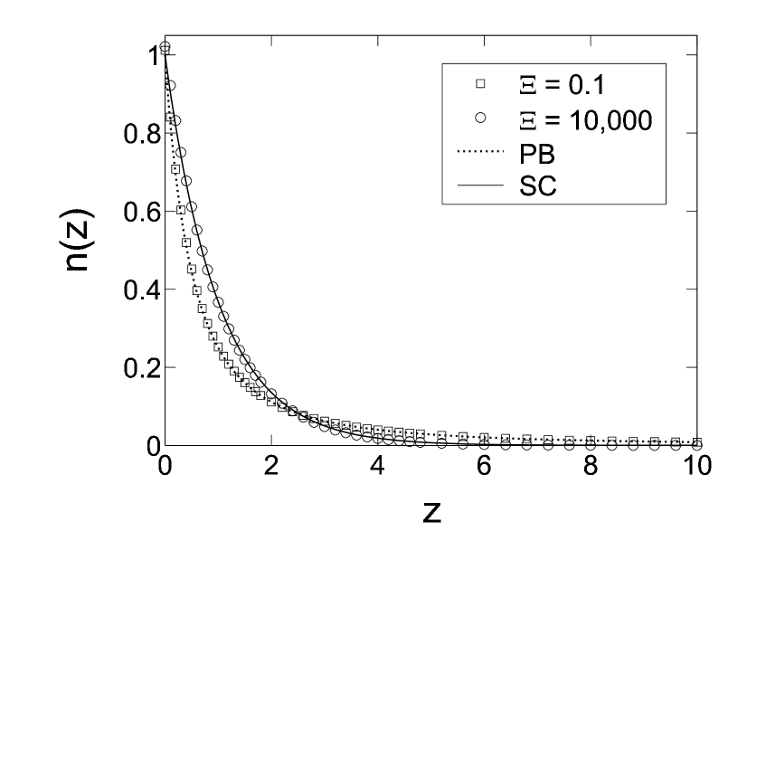
Figure 2: Density profiles, $n(z)$, numerically calculated using the TCMF model of Eqs. (19)-(21), with $\Xi=0.1$ (squares) and $\Xi=$10,000 (circles). The solid lines show the exact asymptotic profiles in the low coupling, $n_{\rm PB}(z)=1/(z+1)^{2}$, and in the strong coupling limit, $n_{\rm SC}={\rm exp}(-z)$.

As a first example we present, in Fig. 2, density profiles obtained numerically from Eqs. (20)-(21) at $\Xi=0.1$ (circles) and at $\Xi=10000$ (squares). The continuous lines are the theoretically predicted profiles at $\Xi\rightarrow 0$, $n_{\rm PB}(z)=1/(z+1)^{2}$, and at $\Xi\rightarrow\infty$, $n_{\rm SC}(z)={\rm exp}(-z)$. The figure demonstrates that the weak coupling and strong coupling limits are reproduced correctly in our approximation. Before presenting further numerical results, we discuss the behavior of our model in the two limits of small and large $\Xi$.

Our discussion is based on the following exact identity:

$$\frac{{\rm d}}{{\rm d}z_{0}}{\rm log}\left[n(z_{0})\right]=-\frac{\rm d}{{\rm d}z_{0}}F(z_{0})=-\left.\frac{\partial}{\partial z}\left<\varphi({\bf r};z_{0})\right>\right|_{\displaystyle{\bf r}=z_{0}\hat{\bf z}}$$ (22)

where $\left\langle\varphi({\bf r};z_{0})\right\rangle$ is the thermally averaged electrostatic potential at ${\bf r}$, when a test charge is fixed at $z_{0}\hat{\bf z}$ (the first argument of $\left\langle\varphi({\bf r};z_{0})\right\rangle$ designates the position ${\bf r}$ where the potential is evaluated, while the second argument designates the position of the test charge, $z_{0}\hat{\bf z}$). In other words, the gradient of ${\rm log}[n(z_{0})]$ is equal to the electrostatic force acting on a test charge positioned at ${\bf r}=z_{0}\hat{\bf z}$. This equation does not involve any approximations and is proved in Appendix B.

Within our approximation, where $F(z_{0})$ is replaced by $F_{\rm PB}(z_{0})$, a similar equation holds (also proved in the Appendix):

$$\frac{{\rm d}}{{\rm d}z_{0}}{\rm log}\left[n(z_{0})\right]=-\frac{\rm d}{{\rm d}z_{0}}F_{\rm PB}(z_{0})=-\left.\frac{\partial}{\partial z}\varphi({\bf r};z_{0})\right|_{\displaystyle{\bf r}=z_{0}\hat{\bf z}}$$ (23)

where $\varphi({\bf r};z_{0})$ is now the solution of Eq. (19). In other words, the gradient of ${\rm log}[n(z_{0})]$ is equal to the electrostatic force experienced by a test charge positioned at ${\bf r}=z_{0}\hat{\bf z}$, evaluated using the mean field equation (19). This quantity,

$$f(z_{0})\equiv\left.\frac{\partial}{\partial z}\varphi({\bf r};z_{0})\right|_{\displaystyle{\bf r}=z_{0}\hat{\bf z}}$$ (24)

will be studied in detail below because of its important role within our model. With this notation the relation between $f(z)$ and $n(z)$ reads:

$$\frac{{\rm d}}{{\rm d}z}{\rm log}\left[n(z)\right]=-f(z)$$ (25)

Using Eq. (25) we can understand why both the weak and strong coupling limits are reproduced correctly in our model:

Weak coupling

In the limit $\Xi\rightarrow 0$,

$$\frac{\partial}{\partial z}\varphi({\bf r};z_{0})\rightarrow\frac{\rm d}{{\rm d}z}\varphi_{\rm PB}(z).$$ (26)

where $\varphi_{\rm PB}(z)$ is the solution of Eq. (19) without a test charge, i.e., setting $\Xi=0$. We note that the potential $\varphi$ (Eq. 19) has three sources: the charge of mobile counterions, $\lambda\theta(z){\rm e}^{-\varphi}$, the uniformly charged plane, and the test charge. Although the potential due to the test charge is infinite at ${\bf r}=z_{0}\hat{\bf z}$, its derivative with respect to $z$ is zero and has no contribution in Eq. (26). Using Eq. (25) we find:

$$\frac{{\rm d}}{{\rm d}z}{\rm log}\left[n(z)\right]=-\frac{{\rm d}}{{\rm d}z}\varphi_{\rm PB}(z)$$ (27)

This equation, together with the normalization requirement for $n(z)$ leads to the result:

$$n(z)=\frac{1}{Z_{0}}{\rm exp}[-\varphi_{\rm PB}(z)]=n_{\rm PB}(z)$$ (28)

Strong coupling

In the strong coupling limit, $\Xi\rightarrow\infty$, a correlation hole forms in the distribution of mobile counterions around the test charge at ${\bf r}=z_{0}\hat{\bf z}$. The structure and size of this hole, as obtained from Eq. (19), will be discussed in detail later. For now it is sufficient to note that the correlation hole gets bigger with increasing $\Xi$. As $\Xi\rightarrow\infty$ the force at $z_{0}\hat{\bf z}$ due to the mobile counterions vanishes, leaving only the contribution of the charged plane: $(\partial/\partial z)\varphi({\bf r};z_{0},\Xi)\rightarrow 1$. Hence in this limit

$$\frac{{\rm d}}{{\rm d}z}{\rm log}\left[n(z)\right]=-1$$ (29)

leading to the strong coupling result:

$$n(z)={\rm exp}(-z)$$ (30)

where the prefactor of the exponent follows from the normalization condition, Eq. (8).

In the rest of this work we will explore predictions of the TCMF model at intermediate coupling, where neither of the two limits presented above is valid. Before proceeding we note that a similar discussion as above, of the weak and strong coupling limits, applies also to the exact theory, because of Eq. (22).

III Numerical Results and Comparison with Simulation

Results for $f(z)$

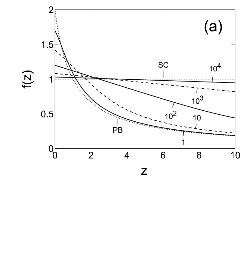
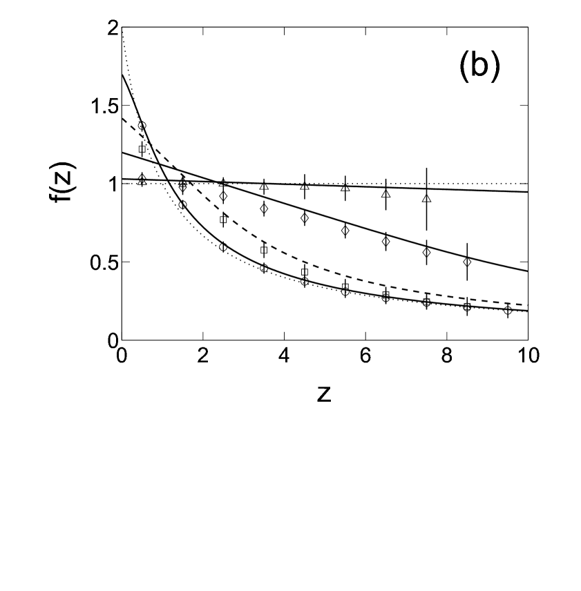
Figure 3: (a) Electrostatic force acting on a test charge, $f(z)$, numerically calculated using the mean field equation (19). Alternating solid and dashed lines show $f(z)$ for $\Xi=1$, 10, $10^{2}$,$10^{3}$, and $10^{4}$. The dotted lines show the PB and SC forms of $f(z)$, $f_{\rm PB}(z)=1/(z+1)$ and $f_{\rm SC}(z)={\rm exp}(-z)$. (b) Comparison of $f(z)$, calculated from Eq. (19) (solid and dashed lines, same as in part (a)), with results from Monte-Carlo simulation MoreiraPrivate , adapted from Ref. MoreiraNetz02 ($\Xi=1$, circles; $\Xi=10$, squares; $\Xi=10^{2}$, diamonds; $\Xi=10^{4}$, triangles). Values of $f(z)$ are obtained from simulation results for $n(z)$ using the exact relation ${\rm d}{\rm log}n(z)/{\rm d}z=-f(z)$. Numerical estimation of the derivative of ${\rm log}\left[n(z)\right]$ results in relatively large error bars, which are shown as vertical lines.

We consider first the behavior of $f(z)$, defined in Eq. (24), close to the charged plate. Fig. 3(a) shows this behavior for $\Xi$ = 1, 10, $10^{2}$, $10^{3}$ and $10^{4}$ (alternating solid and dashed lines). The curves were obtained from a numerical solution of the partial differential equation (PDE), Eq. (19) (see Appendix C for details of the numerical scheme). For comparison the weak coupling (PB) and strong coupling (SC) limits are shown using dotted lines:

$$f_{\rm PB}(z)=\frac{2}{z+1}\ \ \ \ ;\ \ \ \ f_{\rm SC}(z)=1$$ (31)

As $\Xi$ increases $f(z)$ gradually shifts from PB to SC behavior. At $\Xi=10^{4}$, $f(z)$ is very close to $1$ within the range of $z$ shown in the plot, although there is still a noticeable small deviation from unity.

In Fig. 3(b) these results are compared with simulation data (symbols), adapted from Ref. MoreiraNetz02 . The value of $f(z)$ was obtained from the simulation results for $n(z)$ using the relation ${\rm d}{\rm log}[n(z)]/{\rm d}z=-f(z)$ . Qualitatively our results agree very well with simulation. Note especially the gradual decrease of $f(z)$ with increasing $z$ for $\Xi=100$ (diamonds): this value of $\Xi$ is far away from both the weak coupling and the strong coupling limits. The regime where $f(z)$ decreases linearly with $z$ will be further discussed in Sec. IV.1.

It was previously conjectured Netz01 that for all values of $\Xi$ the SC limit is valid close enough to the charged plane. We note, however, that at contact with the plane $f(z)$ is different from unity at small and intermediate values of $\Xi$. Hence it is not very meaningful to define a region close to the plane where the SC limit is valid, unless $\Xi$ is very large. Values of $f(z)$, extracted from simulation data in Fig. 3(b), suggest the same conclusion, i.e., $f(z)$ does not approach unity at contact with the plane. A more accurate measurement of $f(z)$ in the simulation is desirable because the error bars, as obtained in Fig. 3(b), are quite large.

Results for $n(z)$

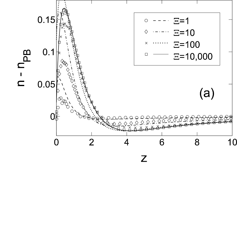
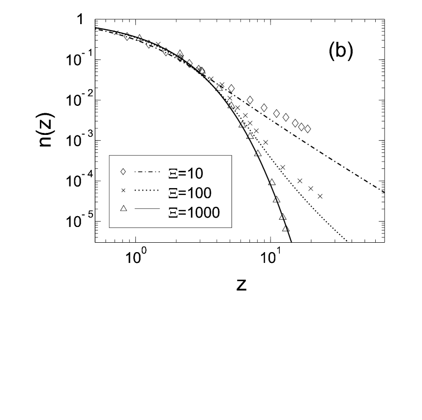
Figure 4: (a) Correction to the PB density profile, $n(z)-n_{\rm PB}(z)$, calculated numerically using the TCMF model, as function of $z$ (lines). For comparison, symbols show the correction obtained from Monte-Carlo simulation MoreiraNetz02 ; MoreiraPrivate . Four values of $\Xi$ are shown (see legend), 1, 10, $10^{2}$, and $10^{4}$. (b) The density profile itself, $n(z)$, on a wider range of $z$ than in part (a) and using logarithmic scales in both axes (lines - TCMF; symbols - MC simulation).

The density profile $n(z)$ can be found numerically by integrating Eq. (25) and use of the normalization condition (8) . Figure 2 already demonstrated that $n(z)$ coincides with the exact profiles, $n_{\rm PB}(z)$ and $n_{\rm SC}(z)$, in the limits of small and large $\Xi$. Figure 4(a) shows the difference between $n(z)$ and $n_{\rm PB}(z)$ for $\Xi=1$, 10, 10², and 10⁴, as calculated numerically in the TCMF model (continuous lines). These results are compared with simulation data (symbols)MoreiraNetz02 ; MoreiraPrivate .

We first observe that the contact theorem is not obeyed in our approximation: $n(0)-n_{\rm PB}(0)=n(0)-1$ is different from zero. This is an undesirable property, because the contact theorem is an exact relation. The contact theorem is obeyed in the TCMF model only in the limits of small and large $\Xi$, where the density profile as a whole agrees with the exact form, and the normalization condition (8) enforces $n(0)$ to be correct. The violation at intermediate values of $\Xi$ is finite, small compared to unity, and peaks at $\Xi$ between 10 and 100. At these values of $\Xi$ the overall correction to PB is quite inaccurate at the immediate vicinity of the charged plate. On the other hand, at $z$ larger than 1 our approximated results agree quite well with simulation for all the values of $\Xi$, as seen in Fig. 4(a).

The violation of the contact theorem in the TCMF model can be traced to a non-zero net force exerted by the ionic solution on itself (see Appendix D). This inconsistency results from the use of a mean field approximation for the distribution of ions around the test charge, while the probability distribution of the test charge itself is given by Eq. (20).

It is possible to evaluate exactly the first order correction in $\Xi$ to the PB density profile in the TCMF model, the details of which are given in Appendix E. This correction turns out to be different from the exact first order correction, which was calculated in Ref. NetzOrland00 using a loop expansion up to one loop order (also shown in the Appendix). It is important to note, however, that the latter correction provides a useful result only for relatively small values of $\Xi$. At $\Xi$ of order 10 and larger TCMF results are much closer to simulation than those of the loop expansion.

Further comparison with simulation is shown in Fig. 4(b). Here we show the density $n(z)$ itself, rather than the difference with respect to $n_{\rm PB}(z)$. The data is shown on a larger range of $z$ than in part (a) and a logarithmic scale is used in order to allow small values of $n(z)$ to be observed far away from the plate. In the range shown the TCMF model agrees semi-quantitatively with simulation.

As a summary of this section we can say that the test charge mean field (TCMF) model captures the essential behavior of the ion distribution at close and moderate distances from the charged plate. Furthermore, all the available data from simulation agrees qualitatively with our approximation’s predictions.

IV TCMF results far away from the charged plate

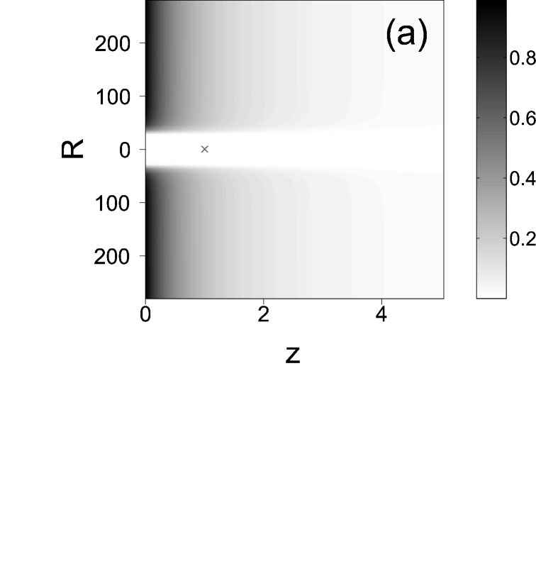
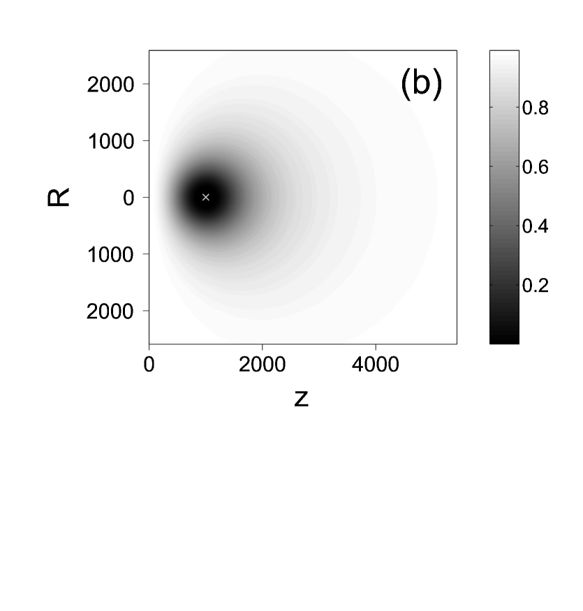
Figure 5: (a) Scaled density of ions around a test charge, positioned at $z_{0}=1$, as obtained from Eq. (19). The cross designates the position of the test charge. In cylindrical coordinates the density is a function only of $z$ (horizontal axis) and $r$ (vertical axis). Darker shading in the plot means larger density (see also the legend on the right). The coupling constant is $\Xi$ = 1,000. For $r$ larger than $\sqrt{\Xi}$ the profile, as function of $z$, quickly converges to the PB profile, $n_{\rm PB}(z)$ (b) A similar plot as in part (a), but the test charge is now at $z_{0}=\Xi$ = 1,000. Here the ratio between the density and the PB profile is shown, rather than the density itself. This ratio is everywhere a number between zero (black) and one (white). The effect of the test charge on the ion distribution is large only within a correlation hole around the test charge, having approximately a spherical shape and a radius of order $\Xi$.

Our analysis of the ion distribution far away from the charged plate is done, at first, strictly within the context of the TCMF model, while a discussion of its relevance to the exact theory is deferred to Sec. V. The main question of interest is whether a transition to PB behavior occurs at sufficiently large $z$, even for large values of $\Xi$.

As a first step we will identify the important length scales characterizing the density distribution. Let us concentrate first on the size of the correlation hole around a test charge. Naively we may expect this size to be of order $\Xi$, due to the form of the bare potential, $\Xi/|{\bf r}-z_{0}\hat{\bf z}|$. A simple argument shows, however, that when the test charge is close to the charged plane the size of the correlation hole is much smaller than $\Xi$. Assume, roughly, that the mobile ion density is zero within a cylindrical shell of radius $R$ around the test charge. The amount of charge depleted from this cylinder is then equal to $R^{2}/2$, since the surface charge per unit area is equal to $1/{2\pi}$ (see Eq. (19)). This depleted charge must balance exactly the charge of the test particle, equal to $\Xi$, yielding a cylinder radius that scales as $\sqrt{\Xi}$ rather than as $\Xi$.

In order to put this argument to test, Fig. 5(a) shows the density of mobile ions calculated from Eq. (19) with a test charge at $z_{0}=1$, having $\Xi$ = 1,000. The shape of the correlation hole is roughly cylindrical and its radius is indeed of order $\sqrt{\Xi}\simeq 30$. The influence of the test charge on its surroundings is very non-linear, with a sharp spatial transition from the region close to the test charge, where the density is nearly zero, to the region further away, where the effect of the test charge is very small. At larger separations from the plate the qualitative picture remains the same, as long as $z_{0}$ is small compared to $\sqrt{\Xi}$ and provided that $\Xi\gg 1$.

A very different distribution of mobile ions is found when $z_{0}$ is of order $\Xi$, as shown in Fig. 5(b). The coupling parameter is the same as in part (a), $\Xi$ = 1,000, but the test charge is now at $z_{0}$ = 1,000. Instead of showing directly the density of mobile ions as in part (a), the figure shows the ratio between this density and $n_{\rm PB}(z)=1/(z+1)^{2}$. This ratio is now very close to unity near the charged plane, where most of the ions are present. It is small compared to unity only within a spherical correlation hole around the test charge, whose size is of order $\Xi$.

The above examples lead us to divide our discussion of the $z$ dependence into two regimes:

IV.1 $z<\sqrt{\Xi}$

In order to justify use of the cylindrical correlation hole approximation within this range, let us assume such a correlation hole and calculate the force acting on the test charge:

$$f(z)\simeq\int_{0}^{\infty}{\rm d}z^{\prime}\,n_{\rm PB}(z^{\prime})\frac{z^{\prime}-z}{\sqrt{\Xi+(z^{\prime}-z)^{2}}}$$ (32)

where $n_{\rm PB}(z^{\prime})$ is given by Eq. (11), the radius of the cylindrical region from which ions are depleted is taken as $\sqrt{\Xi}$, and the expression multiplying $n_{\rm PB}(z^{\prime})$ is the force exerted by a charged sheet having a circular hole of radius $\sqrt{\Xi}$ and positioned in the plane $z^{\prime}$. Figures 6 (a) and (b) show a comparison of this approximation (dashed lines) with that obtained from a full numerical solution of Eq. (19) (solid lines). The coupling parameter is equal to 10,000 in (a) and to 100 in (b). In both cases the approximation works well up to $z_{0}\simeq\sqrt{\Xi}$. In Fig. 6 (c) the force acting on a test charge at contact with the plane, $f(0)$, is shown for five values of $\Xi$ between 1 and 10,000 (symbols), and compared with the approximation of Eq. (32) (solid line). Note that Eq. (32) is not a good approximation when $\Xi$ is of order unity or smaller, since the correlation hole is then small compared to the width of the ion layer.

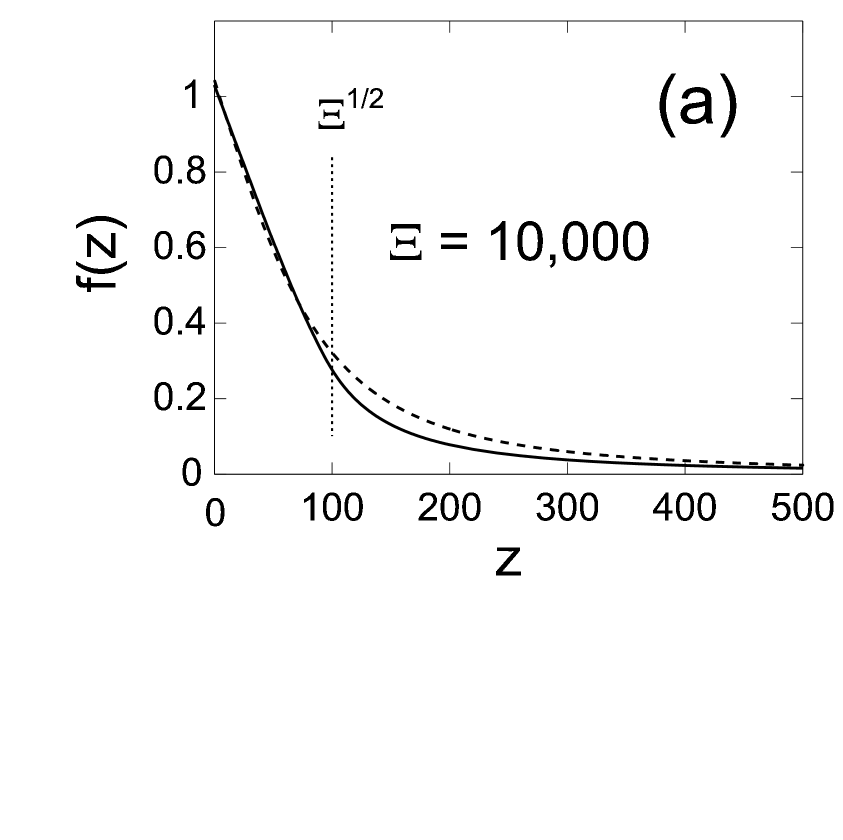
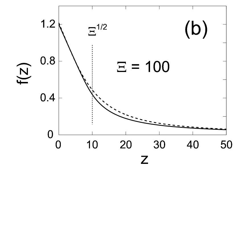
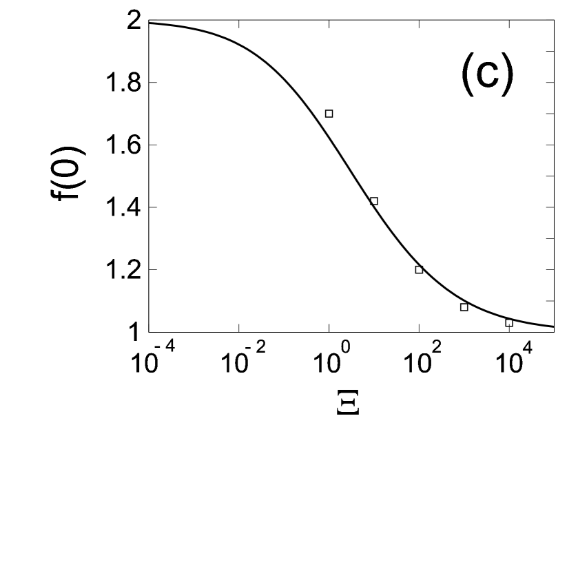
Figure 6: (a), (b) Comparison of the approximation to $f(z)$ given by Eq. (32) (dashed line), with a full numerical solution of the PDE (solid line). The coupling parameter $\Xi$ is equal to 10,000 in (a) and to 100 in (b). Note that the approximation shown in the dashed line is good up to a distance from the plate equal to about $\sqrt{\Xi}$ in both cases. A distance of $\sqrt{\Xi}$ from the charged plate is designated by the vertical dotted lines. Part (c) shows a comparison of $f(0)$ in the approximation given by Eq. (32) (symbols) and in the exact PDE solution (solid line) for a wide range of $\Xi$ values.

IV.2 $z>\sqrt{\Xi}$

When the test charge is far away from the plane, its effect close to the charged plate is small, suggesting that a linear response calculation may be applicable:

$$f(z)=f_{\rm PB}(z)+\Xi f_{1}(z)$$ (33)

The first term in this equation is the PB value of $f(z)$, while $f_{1}(z)$ can be calculated using previous results of Ref. NetzOrland00 :

$$f_{1}(z) = \frac{1}{2}\frac{{\rm d}g(z)}{{\rm d}z}=\frac{1}{4(z+1)^{3}}\times{\Big{\{}}8z$$ (34)

$$- (1+i){\rm e}^{(1-i)z}\left[1-z+(1-2i)z^{2}+z^{3}\right]$$

$$\times E_{1}\left[(1-i)z\right]$$

$$- (1-i){\rm e}^{(1+i)z}\left[1-z+(1+2i)z^{2}+z^{3}\right]$$

$$\times E_{1}\left[(1+i)z\right]{\Big{\}}}$$

where $g(z)$ was defined in Ref. NetzOrland00 and is given by Eq. (79), and $E_{1}(z)$ is the exponential-integral function AStegun . We prove the first equality of Eq. (34) in Appendix E. Figure 7 shows $f_{1}(z)$ (solid line) together with its asymptotic form for large $z$ (dashed line),

$$f_{1}(z)\simeq\frac{3}{4z^{2}}\ \ \ ,\ \ \ z\gg 1$$ (35)

Note that the asymptotic form of $\Xi f_{1}(z)$ has the same $z$ dependence as the electrostatic force exerted by a metallic surface, equal to $\Xi/(4z^{2})$ in our notation, but the numerical prefactor is different.

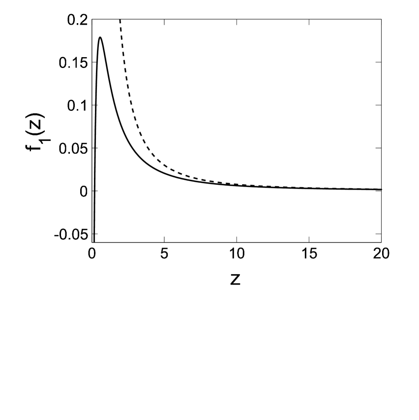
Figure 7: First order (linear) term in an expansion of $f(z)$: $f(z)=f_{\rm PB}(z)+\Xi f_{1}(z)+\ldots$, Eq. (34), as obtained from the loop expansion of Ref. NetzOrland00 . The dashed line shows the asymptotic form of $f_{1}(z)$ at large $z$, $f_{1}(z)\simeq 3/(4z^{2})$.

Although the influence of the test charge is small near the surface, its influence on ions in its close vicinity is highly non-linear and definitely not small. Hence the applicability of Eq. (33) is far from being obvious when $\Xi$ is large. We check this numerically by calculating $f(z)-f_{\rm PB}(z)$ and comparing with $\Xi f_{1}(z)$. The results are shown in Fig. 8(a), for 5 values of $\Xi$: 1, 10, $10^{2}$, $10^{3}$, and $10^{4}$.

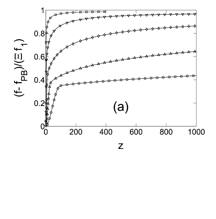
Figure 8: Comparison between the correction to $f(z)$ relative to $f_{\rm PB}(z)$, with the linearized expression $\Xi f_{1}(z)$. In (a) the ratio $[f(z)-f_{\rm PB}(z)]/[\Xi f_{1}(z)]$ is shown as function of $z$ for five different values of $\Xi$: 1, 10, 10², 10³, and 10⁴ (see legend in part (b); symbols show the same quantity as the solid line and are displayed in order to distinguish between the five lines). The ratio approaches unity at $z$ much larger than $\Xi$. In (b) the same data as in (a) is shown as function of $z/\Xi$, leading to an almost perfect collapse of the five data sets on a single curve.

For each value of $\Xi$ the ratio $(f-f_{\rm PB})/(\Xi f_{1})$ (shown in the plot) approaches unity as $z$ is increased, showing that Eq. (33) does become valid at sufficiently large $z$. The approach is, however, rather slow: a value close to unity is reached only when $z\gg\Xi$. At $z=\Xi$ the ratio is approximately equal to 0.6 in all five cases. We conclude that the linear approximation of Eq. (33) is applicable only for $z\gg\Xi$. Note that at these distances from the charged plate the linear correction itself is very small compared to the PB term,

$$\frac{\Xi f_{1}(z)}{f_{\rm PB}(z)}\simeq\frac{3\Xi}{4z^{2}}\frac{z+1}{2}\simeq\frac{3}{8}\frac{\Xi}{z}\ll 1$$ (36)

where we also assumed that $z\gg 1$ and used Eq. (35).

Further insight on the results shown in Fig. 8(a) is obtained by noting that all of them approximately collapse on a single curve after scaling the $z$ coordinate by $\Xi$. This curve, denoted by $h(z/\Xi)$, is shown in Fig. 8(b):

$$f(z)-f_{\rm PB}(z)\simeq\Xi f_{1}(z)\times h\left(\frac{z}{\Xi}\right)$$ (37)

In order to demonstrate at what range of $z$ values this scaling result is valid the same data is shown in Fig. 9 using a logarithmic scale in the horizontal ($z/\Xi$) axis. It is then seen clearly that (37) holds for $z/\Xi$ larger than a minimal value, which is proportional to $\Xi^{-1/2}$. The vertical arrows designate $z/\Xi=1.5/\sqrt{\Xi}$ for each value of $\Xi$, approximately the point where the scaling becomes valid. Returning to consider $z$ itself, we conclude that (37) holds for $z\gtrsim 1.5\sqrt{\Xi}$. This result justifies the separation of the $z$ dependence into two regimes, $z<\sqrt{\Xi}$ and $z>\sqrt{\Xi}$.

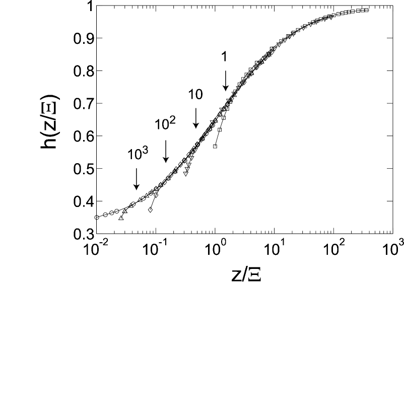
Figure 9: Same data as in Fig. 9(b), shown using a logarithmic scale in the horizontal (z/$\Xi$) axis. The approximated collapse of the different data sets, corresponding to different values of $\Xi$, is seen to be valid only in the regime $z\gtrsim\sqrt{\Xi}$. The vertical arrows mark $z=1.5\sqrt{\Xi}$ for $\Xi=1$, 10, 10², and 10³, above which the scaling (3) is approximately valid.

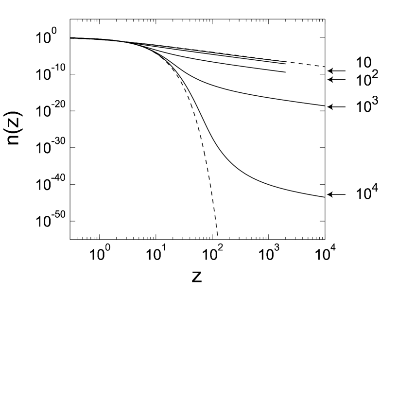
Figure 10: Scaled ion density, $n(z)$ calculated using the TCMF model, shown for five different values of $\Xi$ (solid lines, top to bottom): 1, 10, 10², 10³, and 10⁴. A logarithmic scale is used on both axis, allowing the behavior far away from the charged plate to be seen. The dashed lines show $n_{\rm PB}(z)$ (upper dashed line) and $n_{\rm SC}(z)$ (lower dashed line). At $z\gg\Xi$ the density profile is proportional to $n_{\rm PB}(z)$, with a prefactor whose logarithm scales as $\sqrt{\Xi}$. To demonstrate this the horizontal arrows mark the value of ${\rm exp}(-0.8\sqrt{\Xi})\times n_{\rm PB}({10^{4}})$ for $\Xi=10$, $10^{2}$, $10^{3}$, and $10^{4}$. The prefactor 0.8 is an approximate fitting parameter.

We finally turn to consider the ion density $n(z)$. Using Eqs. (35) and (37) we can write

$$-\frac{\rm d}{{\rm d}z}n(z)=f(z)\simeq f_{\rm PB}(z)+\frac{1}{\Xi}\cdot\frac{3}{4}\left(\frac{z}{\Xi}\right)^{-2}h\left(\frac{z}{\Xi}\right)$$ (38)

which leads, upon integration, to the approximate scaling result,

$$n(z)\simeq c_{0}(\Xi)\frac{1}{(z+1)^{2}}\eta\left(\frac{z}{\Xi}\right)$$ (39)

where

$${\rm log}[\eta(u)]=-\frac{3}{4}\int_{u}^{\infty}{\rm d}u^{\prime}\,\frac{h(u^{\prime})}{u^{\prime 2}}$$ (40)

The prefactor $c_{0}(\Xi)$ depends, through the normalization condition, on the behavior of $n(z)$ close to the charged plane where the scaling form of Eq. (39) is not valid. Equation (39) is indeed validated by the numerical data and applies for $z\gtrsim\sqrt{\Xi}$ and $\Xi\gg 1$.

The density itself, $n(z)$, is plotted in Fig. 10 using a semi-logarithmic scale, for $\Xi$ = 1, 10, 10², 10³, and $10^{4}$. At $z\gg\Xi$ $n(z)$ is proportional to $n_{\rm PB}(z)$, as expected from Eq. (39). The prefactor $c_{0}$ is extremely small for large $\Xi$. We recall that $c_{0}$ is mainly determined by the behavior close to the charged plane, where $f(z)$ is of order unity up to $z\lesssim\sqrt{\Xi}$. Following this observation we can expect ${\rm log}[c_{0}(\Xi)]$ to scale roughly as $\sqrt{\Xi}$. This estimate is validated by the numerical results and is demonstrated in the figure using the horizontal arrows. For $\Xi=10$, $10^{2}$, $10^{3}$, and $10^{4}$ these arrows show an estimate for $n(z)$ at $z=10^{4}$, given by

$$n_{\rm PB}(z)\times{\rm exp}(-0.8\sqrt{\Xi})$$

in very good agreement with the actual value of $n$.

V Further Discussion

At this point we may ask to what extent our results represent the behavior of $n(z)$ in the exact theory. Before discussing this question we turn our attention for a moment to the system that our problem was mapped into in Eq. (19) – that of a single ion of valence $\Xi$ in contact with a charged plane and its monovalent counterions. The results of Sections III and IV can be regarded as exact for such a system, provided that the monovalent ions are weakly correlated (having, by themselves, a small coupling parameter as determined from their charge and that of the planar surface). These results are thus of direct relevance to the interaction of a large multivalent macroion with a charged surface that is immersed in a weakly correlated solution of counterions.

Returning to the original question, we separate our discussion according to the scaling results of the numerical analysis:

V.1 $z<\sqrt{\Xi}$

When $\Xi$ is very large a test charge at $z<\sqrt{\Xi}$ is essentially decoupled from the rest of the ionic solution, feeling only the force exerted by the charged plane. This is the reason why an exponential decay, $n(z)\sim{\rm exp}(-z)$, is obtained in our model, as well as in simulation and in the perturbative strong coupling expansion of Ref. Netz01 . However, at intermediate values of $\Xi$ such as 10, 100, or 1000 our results show that this exponential decay is only a rough approximation. The decoupling of a test charge from the rest of the ions is only partial, even at $z=0$, leading to a value of $f(z)$ that is (i) larger than unity at $z=0$ and (ii) considerably smaller than unity at $z=\sqrt{\Xi}$. Both of these predictions are validated by simulation, as shown in Fig. 3(b).

The quantitative agreement in $f(z)$ between our model and simulation is surprisingly good, considering that the ionic environment surrounding the test charge is different in our approximation, compared to the exact theory. This good agreement can be attributed to the correct length scales that characterize the approximate ionic environment: $\sqrt{\Xi}$ in the lateral direction, and 1 in the transverse direction. Indeed, in the lateral direction our results can be compared with pair distributions that were obtained in Monte-Carlo simulation MoreiraNetz02 . The pair distributions found in the simulation are characterized by a strong depletion within a correlation hole having diameter of order $\sqrt{\Xi}$, in great similarity to Fig. 5(a). What is not captured by our approach is that multiple maxima and minima exist at $\Xi\gtrsim 100$ . Nevertheless, even at the very large coupling parameter value $\Xi=10^{4}$ these oscillations decay quite rapidly with lateral distance, and we can still say that the TCMF model captures the most significant feature of the pair distribution (namely, the structure of the correlation hole).

V.2 $z>\sqrt{\Xi}$

Throughout most of this section we concentrate on the case $z>\Xi$, while a short discussion of the range $\sqrt{\Xi}<z<\Xi$ is presented at the end of this section.

Our model predicts a transition to algebraic decay of $n(z)$ at $z\gtrsim\Xi$. Similar predictions were made in Ref. Shklovskii and in Ref. MoreiraNetz02 , where it was estimated that mean field results are valid for $z>\Xi{\rm log}\Xi$ based on a perturbative expansion around mean field. There are currently no available results from simulation in this regime.

A mean field behavior is obtained in our model in the sense that

$$f(z)\simeq f_{\rm PB}(z)=\frac{1}{z+1}$$ (41)

decays as $1/z$ for large $z$. Nevertheless the finer details in our results do not match the form predicted by PB theory. The starting point for the following discussion is an hypothesis that sufficiently far from the plate the exact density follows a PB form,

$$n_{\rm asym}(z)=\frac{1}{(z+b)^{2}}$$ (42)

where $b$ (or $\mu b$ in the original, non-scaled coordinates) is an effective Gouy-Chapman length, characterizing the ionic solution far away from the plate.

The asymptotic density profile found in our approximation, $n(z)=c({\Xi})/(z+1)^{2}$, is different from Eq. (42). To understand this difference let us explain first the asymptotic behavior of $f(z)$: it decays in the TCMF model as $1/(z+1)$ because beyond the correlation hole the test charge is surrounded by an ion density of the form $n_{\rm PB}=1/(z+1)^{2}$. This form is different from the profile $n(z)$ that is eventually obtained by integrating $f(z)$ – an inconsistency which is the source of the difference between $f(z)$ in our approximation and the hypothesized form $f(z)\sim 1/(z+b)$ (see also the discussion in Appendix D).

The behavior of our approximate $f(z)$ leads to a decay of $n(z)$ of the form $1/(z+1)^{2}$. The normalization condition for $n(z)$ is then enforced through a small prefactor $c({\Xi})$. In comparison, in the hypothesized form (42) the prefactor must be 1 and the normalization is achieved by a large value of $b$. Note that $b$ must be an extremely large number for large values of $\Xi$: due to the exponential decay of $n(z)$ at $z\lesssim\sqrt{\Xi}$ the logarithm of $b$ must be at least of order $\sqrt{\Xi}$.

Further insight on the behavior at $z>\Xi$ can be obtained using the exact equation (22):

$$\frac{\rm d}{{\rm d}z}{\rm log}\left[n(z)\right]=-f(z)$$ (43)

where $f(z)$ is now the mean (thermally averaged) electrostatic force acting on a test charge at distance $z$ from the plate, in the exact theory.

For the mean field form $n_{\rm asym}(z)$ to be correct, the contribution to $f(z)$ coming from the influence of the test charge on its environment must be small compared to the mean field force, which is given by $1/(z+b)$. Following our results from the previous section, the former quantity is given by ${\alpha}\Xi/z^{2}$, where $\alpha$ is of order unity. Using the mean field equation (19) we obtained $\alpha=3/4$; in the exact theory, and for large $\Xi$, where ions form a much more localized layer close to the plane than in mean field, it is plausible that $\alpha=1/4$, as in the force acting on a test charge next to a conducting surface Shklovskii ; MoreiraNetz02 . In any case, for Eq. (42) to represent correctly the decay of $n(z)$ we must have

$$\frac{\alpha\Xi}{z^{2}}<\frac{1}{z+b}$$ (44)

leading to the result $z\gtrsim(\Xi b)^{1/2}$ which is exponentially large due to $b$. Up to this crossover distance the decay of $n(z)$ is dominated by the correlation-induced interaction with the ions close to the plate.

We conclude that for a very large range of $z$ values the decay of $n(z)$ must be different from Eq. (42). At the same time, a mean field argument is probably applicable, because the density of ions is very small in this regime: we may presume that the contribution to $f(z)$ can be divided into two parts – one part, coming from ions far away from the plate, which is hardly influenced by the test charge; and a second part, coming from ions close to the charged plate, where the test charge influence on $f(z)$ is given by $\alpha\Xi/z^{2}$. This reasoning leads to the following differential equation for $n(z)$:

$$\frac{{\rm d}^{2}}{{\rm d}z^{2}}{\rm log}[n(z)]=2n(z)+\frac{2\alpha\Xi}{z^{3}}$$ (45)

whose detailed derivation is given in Appendix F. By defining $n(z)={\rm exp}(-\phi+\alpha\Xi/z)$ Eq. (45) is recast in the form:

$$\frac{{\rm d}^{2}\phi}{{\rm d}z^{2}}=-2{\rm exp}\left(-\phi+\frac{\alpha\Xi}{z}\right)=-2n(z)$$ (46)

showing that mean field theory is applicable, but an external potential $-\alpha\Xi/z$, coming from the ions close to the plate, must be included in the PB equation. In practice, for large $\Xi$ this equation will lead to a decay of the form $n(z)\sim{\rm exp}(\alpha\Xi/z)$ as suggested also in Refs. Shklovskii ; MoreiraNetz02 , while a crossover to an algebraic decay will occur only at a distance of at least $\left[\Xi{\rm exp}(\sqrt{\Xi})\right]^{1/2}$ where Eq. (44) has been used and prefactors of order unity, inside and outside the exponential, are omitted. A numerical solution of Eq. (46) may be useful in order to describe the ionic layer at intermediate values of $\Xi$ (of order 10 - 100), where both mean field and correlation-induced forces are of importance at moderate distances from the plate. In order to test this idea quantitatively more data from simulation is required.

Finally we discuss the case where $z>\sqrt{\Xi}$ but $z$ is not large compared to $\Xi$. Let us also assume that $\Xi$ is very large, so that most of the ions are much closer to the plate than a test charge fixed at $z\hat{\bf z}$. Within the TCMF model the effect of the test charge on ions close to the plate is nonlinear, leading to the scaling result of Eq. (37). Similarly, in the exact theory it is not clear whether the correlation-induced force acting on the test charge is of the form $\alpha\Xi/z^{2}$, since the effect of the test charge on ions close to the plate is not a small perturbation. Hence we believe that the relevance of Eq. (46) for $z<\Xi$, and the behavior of $f(z)$ in this regime, merit further investigation .

VI Conclusion

In this work we showed how ion correlation effects can be studied by evaluating the response of the ionic solution to the presence of a single test particle. Although we calculated this response using a mean field approximation, we obtained exact results in the limits of small and large $\Xi$, and qualitative agreement with simulation at intermediate values.

The approach taken in this work demonstrates that for highly correlated ionic liquids it is essential to treat the particle charge in a non-perturbative manner. Once a single ion is singled out, even a mean field approximation applied to the other ions provides useful results. This scheme, called the test-charge mean field (TCMF) model, provides a relatively simple approximation, capturing the essential effects of strong correlations – to which more sophisticated treatments can be compared.

Technically what is evaluated in this work is the ion-surface correlation function. Consideration of correlation functions of various orders leads naturally to liquid state theory approximations BlumHenderson , some of which are very successful in describing ionic liquids KjelMar . In particular these approximations usually treat the ion-ion correlation function in a more consistent manner than the approximation used in this work, thus possibly alleviating some of the undesirable features of the TCMF model presented here, such as the violation of the contact theorem. The main advantage of the TCMF model is its simplicity, allowing the behavior of $n(z)$ to be understood in all the range of coupling parameter values in terms of $f(z)$, the force acting on a test charge. Furthermore, the exact equation (22), which does not involve any approximation, is a useful tool in assessing correlation effects – as was done, for example, in this work in the end of Sec. V.

It will be useful to summarize the main results obtained in this work. First, the exact equation (22) provides a simple explanation of the exponential decay of the density profile in the strong coupling limit. In light of this equation, exponential decay is expected as long as the test charge is decoupled from the rest of the ionic solution. Note that there is no necessity for long range order to exist in order for the exponential decay to occur, as was emphasized also in Ref. Shklovskii . Indeed, within our TCMF model the ion distribution around a test charge does not display any long range order (see Fig. 5(a)) and yet simulation results, in particular in the strong coupling limit, are recovered very successfully.

Second, the characteristic size of the correlation hole around an ion close to the plane, $\sqrt{\Xi}$, plays an important role in determining the density profile. For very large $\Xi$ the profile decays exponentially up to $z\lesssim\sqrt{\Xi}$, beyond which a crossover to a less rapid decay occurs. For intermediate values of the coupling parameter $z=\sqrt{\Xi}$ is still an approximate boundary between regimes of different behavior of $n(z)$, but the density profile at $z<\sqrt{\Xi}$ does not decay in the simple exponential form ${\rm exp}(-z)$. In this sense one cannot speak of a region close to the plate where strong coupling results are valid.

For $z\gtrsim\Xi$ our approximation predicts a transition to an algebraic decay of $n(z)$, of the form $c(z)/(z+1)^{2}$, where the prefactor $c(z)$ is exponentially small for large $\Xi$. A different asymptotic behavior of the form $1/(z+b)^{2}$ is probably valid at very large $z$, but is not predicted by the TCMF model. Arguments presented in Sec. V, based on the exact equation (22), lead to the conclusion that for large $\Xi$ the latter form (with a constant value of $b$) can only be valid at extremely large values of $z$, while suggesting that at all distances from the plate larger than $\Xi$ a modified mean field equation, Eq. (46), is valid. This equation, matched with the behavior of the ion distribution close to the charged plate, ultimately determines the value of the effective Gouy-Chapman length $b$.

Finally, as a by-product of the analysis of Sec. IV, we obtain scaling results for the interaction of a high-valent counterion with a charged plane immersed in a weakly correlated ionic liquid. All the results of Sec. IV and in particular the scaling form (37), valid for $z\gtrsim\sqrt{\Xi}$, can be regarded as exact in such a system.

Our approach can be easily generalized to more complicated geometries than the planar one, although the practical solution of the PB equation with a test charge may be more difficult in these cases. Other natural generalizations are to consider non-uniformly charged surfaces and charged objects in contact with a salt solution. Beyond the TCMF approximation of Eqs. (19), (20), and (21), the exact equation (22) always applies and can be a very useful tool for assessing correlation effects near charged macromolecules of various geometries.

We conclude by noting that important questions remain open regarding the infinite planar double layer, which is the most simple model of a charged macroion in solution. One such issue, on which the present work sheds light, is the crossover from a strongly coupled liquid close to the charged plate to a weakly correlated liquid further away. In particular, the precise functional dependence of the effective Gouy-Chapman length $b$ on $\Xi$ is still not known. More simulation results, in particular at large distances from the charged plate, and a direct evaluation of $f(z)$ from simulation, may be useful in order to gain further understanding and to test some of the ideas presented in this work. Another important issue, which has not been addressed at all in the present work, is the possible emergence of a crystalline long range order parallel to the plane at sufficiently large values of the coupling parameter. Although plausible arguments have been presented for the occurrence of such a phase transition at $\Xi\gtrsim 3\times 10^{4}$ Shklovskii , its existence has not been proved.

Appendix A Mean field free energy

In this appendix we show how the mean field free energy (18) is obtained as an approximation to $F(z_{0})$, Eq. (14). We start from a general expression for the grand canonical potential of an ionic solution interacting with an external and fixed charge distribution $\sigma({\bf r})$. In the mean field approximation BurakAndelman00 ; NetzOrland00 ,

$$\Omega = \int{\rm d}^{3}{\bf r}\,\left\{-\frac{1}{8\pi l_{B}q^{2}}\left[{\bf\nabla}\phi({\bf r})\right]^{2}+\frac{\sigma({\bf r})\phi({\bf r})}{q}\right.$$ (47)

$$-\left.\lambda\Theta({\bf r}){\rm e}^{-\phi({\bf r})}\right\}$$

where $q$ is the valency of the ions, $\lambda$ is the fugacity, $\Theta({\bf r})$ is equal to $1$ in the region accessible to the ions and to zero elsewhere (equal in our case to $\theta(z)$, the Heaviside function), and $\Omega$ is given in units of $k_{B}T$. Requiring an extremum with respect to $\varphi$, the reduced electrostatic potential, yields the PB equation which determines the electrostatic potential and the actual value of $\Omega$. We use equation (47), which is given in the grand-canonical ensemble, because it is widely used in the literature BurakAndelman00 ; NetzOrland00 . In Ref. NetzOrland00 Eq. (47) is derived systematically as the zero-th order term in a loop expansion of the exact partition function.

Inspection of Eq. (14) shows that it describes the free energy of an ionic solution interacting with an external charge distribution having the following parameters,

$$\begin{array}[]{llll}\mbox{valency}&q&=&\sqrt{\Xi}\\ \mbox{Ext. potential \ }&\sigma({\bf r})&=&{\displaystyle\frac{1}{\sqrt{\Xi}}\left[-\frac{1}{2\pi}\delta(z)+\Xi\delta({\bf r}-z_{0}{\bf\hat{z})}\right]}\\ \mbox{Bjerrum length}&l_{B}&=&1\end{array}$$ (48)

In the second line (external potential) the first term comes from the uniformly charged plate and the second term comes from the fixed test charge. Plugging these values in Eq. (47) yields,

$$\Omega = \frac{1}{\Xi}\int{\rm d}^{3}{\bf r}\left\{-\frac{1}{8\pi}({\bf\nabla}\varphi)^{2}-\lambda\theta(z){\rm e}^{-\varphi}\right.$$ (49)

$$+ \left.\varphi\left[-\frac{1}{2\pi}\delta(z)+\Xi\delta({\bf r}-z_{0}{\bf z})\right]\right\}$$

In order to obtain Eq. (18) two modifications are required. First, we need to return to the canonical ensemble by adding $\mu N$ to $\Omega$, where $N$ is the total number of ions. Noting that $\mu={\rm log}\lambda$ and that from charge neutrality $qN=-\int{\rm d}^{3}{\bf r}\sigma({\bf r}),$ this modification yields the extra term that is proportional to $\log\lambda$ in Eq. (18). Second, we note that $\Omega$ includes the Coulomb self-energy of the charged plane and of the test charge. This infinite term does not depend on $z_{0}$ and should be subtracted from $\Omega$ since it is not included in the definition of $F(z_{0})$, Eq. (14).

We finally note that the results of this Appendix can also be obtained directly from the canonical partition function, as expressed by Eq. (14).

Appendix B Derivation of Identity (23)

We would like to evaluate the variation $\delta F_{\rm PB}(z_{0})/\delta z_{0}$, where $F_{\rm PB}$ is given by Eq. (18). Note that $\varphi$ itself depends on $z_{0}$. However the first derivative of $F_{\rm PB}$ with respect to $\varphi({\bf r})$ is zero. Hence the only contribution to $\delta F_{\rm PB}/\delta z_{0}$ comes from the explicit dependence on $z_{0}$:

$$\frac{\delta F_{\rm PB}[z_{0}]}{\delta z_{0}} = \frac{1}{\Xi}\int{\rm d}^{3}{\bf r}\,(\varphi-{\rm log}\lambda)\Xi\frac{\partial}{\partial z_{0}}\delta({\bf r}-z_{0}{\bf\hat{z}})$$ (50)

$$= -\left.\frac{\partial\varphi}{\partial z}\right|_{\displaystyle{\bf r}=z_{0}\hat{\bf z}}$$

It is also instructive to derive this identity within the exact theory. Equation (14) can be written as follows:

$${\rm exp}[-F(z_{0})]=\frac{1}{(N-1)!}\int\prod_{i=1}^{N-1}{\rm d}^{3}{\bf r}_{i}\,{\rm exp}\left(-H_{z_{0}}\{{\bf r}_{i}\}\right)$$ (51)

where the $N$-th charge is fixed at ${\bf r}=z_{0}\hat{\bf z}$:

$$H_{z_{0}}\{{\bf r}_{i}\}=-z_{0}-\sum_{i=1}^{N-1}z_{i}-\sum_{i=1}^{N-1}\frac{\Xi}{\left|{\bf r}_{i}-z_{0}\hat{\bf z}\right|}-\sum_{j>i}\frac{\Xi}{\left|{\bf r}_{i}-{\bf r}_{j}\right|}$$ (52)

Differentiating with respect to $z_{0}$ yields:

$$\frac{\delta F(z_{0})}{\delta z_{0}}=-\left<\frac{\partial H_{z_{0}}}{\partial z_{0}}\right>=-\left<-1+\sum_{i=1}^{N-1}\frac{\Xi(z_{0}-z_{i})}{\left|{\bf r}_{i}-z_{0}{\bf\hat{z}}\right|^{3}}\right>$$ (53)

where the averaging is performed over all configurations of the $N-1$ ions with the weight ${\rm exp}(-H_{z_{0}}\{{\bf r}_{i}\})$. This quantity is the mean electrostatic field acting on a test charge at $z_{0}{\bf\hat{z}}$.

Appendix C Numerical scheme

Numerically solving a non-linear PDE such as (19) requires careful examination of the solution behavior. The purpose of this section is to explain the numerical scheme used in this work, and in particular the parameters required to obtain a reliable solution.

Finite cell

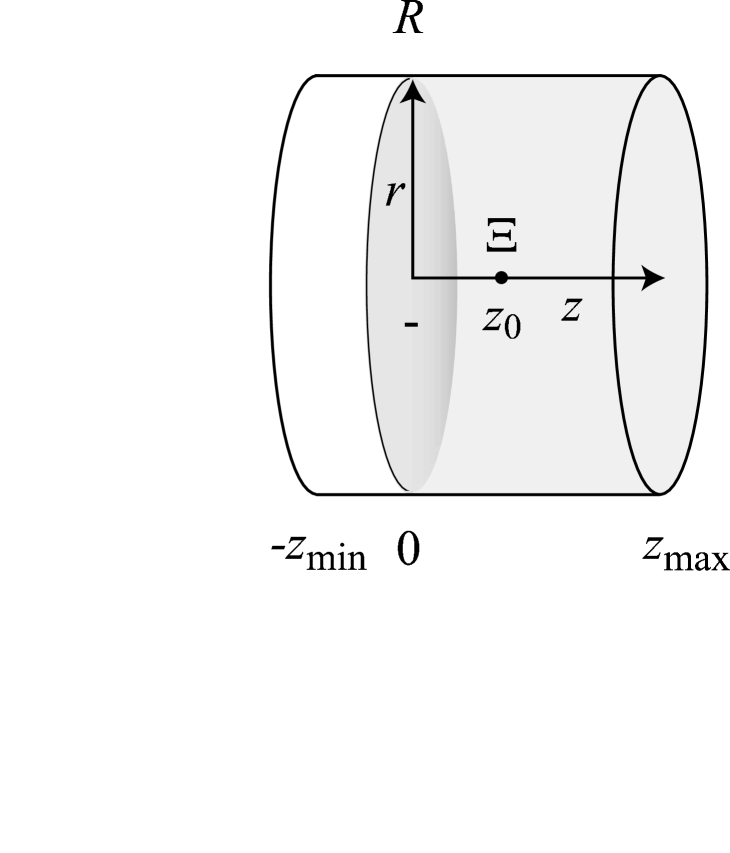
Figure 11: Schematic illustration of the setup used to solve numerically the PDE (19). The equation is solved in a finite cylindrical cell, extending from $-z_{\rm min}$ to $z_{\rm max}$ in the $z$ axis and from $0$ to $R$ in the $r$ axis. The charged plane is at $z=0$ and ions are only present for $z>0$. Neumann boundary conditions $({{\bf\nabla}\varphi}\cdot\hat{\bf n}=0)$ are imposed at the cell boundaries. The test charge is at ${\bf r}=z_{0}\hat{\bf z}$

We solve Eq. (19) as a two dimensional problem in the coordinates $r$ and $z$, making use of the symmetry of rotation around the $z$ axis. The problem is defined within a finite cell of cylindrical shape, shown schematically in Fig. 11. The negatively charged plate is at $z=0$ and ions are only allowed in the region $z>0$, marked as the gray-shaded region in the plot.

We impose a boundary condition of zero electrostatic field,

$${\rm\nabla}\varphi\cdot\hat{\bf n}=0,$$ (54)

at the cell boundaries: $z=-z_{\rm min}$, $z=z_{\rm max}$, and $r=R$. The cell size, as determined by these boundaries, must be sufficiently large, as will be further discussed below.

In the numerical solution it is necessary to solve $\varphi$ for the electrostatic potential at positive as well as negative $z$ . Note that a boundary condition such as (54) at $z=0$ would correspond to zero dielectric constant at $z<0$, while we are interested in the case of continuous dielectric constant across the plate.

Differential equation

The source term in Eq. (19) diverges at $z=0$ and at ${\bf r}=z_{0}\hat{\bf z}$. We avoid this difficulty by shifting the potential:

$$\varphi=\psi+|z|+\frac{\Xi}{|{\bf r}-z_{0}\hat{\bf z}|}$$ (55)

and solving for $\psi$, which is the potential due only to the mobile ions. The equation for $\psi$,

$${\bf\nabla}^{2}\psi=-4\pi\lambda\theta(z){\rm exp}\left(-\psi-z-\frac{\Xi}{|{\bf r}-z_{0}\hat{\bf z}|}\right)$$ (56)

is solved with a Neumann boundary condition for $\psi$, derived from Eqs. (54) and (55). Note that, unlike $\varphi$, $\psi$ is well behaved at $z_{0}\hat{\bf z}$. The nonlinear equation (56) can be solved by iterative solution of a linear equation (see, for example, Harries ; CarnieChan94 ),

$${\bf\nabla}^{2}\psi_{n} = -4\pi\lambda\theta(z){\rm exp}\left(-\psi_{n-1}-z-\frac{\Xi}{|{\bf r}-z_{0}\hat{\bf z}|}\right)$$ (57)

$$\times \left[1-\left(\psi_{n}-\psi_{n-1}\right)\right]$$

where $\psi_{n}$ represents the $n$-th iteration.

Grid and solution method

In the coordinates $r$,$z$ the cylindrical cell is a rectangular domain,

$$[0,R]\times[-z_{\rm min},z_{\rm max}].$$

We use bi-cubic Hermite collocation Houstis in this domain in order to translate the PDE into a set of linear algebraic equations on a grid. These equations are then solved using Gauss elimination with scaled partial pivoting. Storing the band matrix representing the linear equations requires approximately $48\times N_{r}^{2}\times N_{z}$ memory cells, where $N_{r}$ and $N_{z}$ are the number of grid points in the $r$ and $z$ directions, respectively Houstis . Because this number can be very large, it is essential to use a variably spaced grid in both of the coordinates. We use the following scheme:

r coordinate: In the absence of a test charge, an arbitrarily coarse grid can be used in the $r$ direction, due to the translational symmetry parallel to the charged plane. In our case (where a test charge is present) the grid spacing is determined by the distance from the test charge, as follows,

$$\frac{{\rm d}n}{{\rm d}r}=\frac{n_{r}}{r+r_{\rm grid}},$$ (58)

where $n_{r}$ and $r_{\rm grid}$ are two fixed parameters, while $n$ stands for the grid point index and ${\rm d}n/{\rm d}r$ is the number of grid points per unit increment of the radial coordinate. This spacing is approximately uniform up to the threshold $r_{\rm grid}$, whereas for $r\gg r_{\rm grid}$ it is proportional to $1/r$. The grid points are then of the form

$$r_{n}=r_{\rm grid}\times\left[{\rm exp}\left(\frac{n}{n_{r}}\right)-1\right]$$ (59)

In practice $r_{\rm grid}$ is chosen approximately proportional to $\sqrt{\Xi}$, in order to allow the structure of the correlation hole to be represented faithfully.

z coordinate: In this coordinate the grid spacing is influenced by the distance from the charged plate as well as the distance from the test charge. We describe separately the spacing determined from each of these two criteria; the actual grid is obtained by using the smaller of the two spacings at each point.

(i) Distance from the plate: we use a grid spacing proportional to the derivative of $\varphi_{\rm PB}(z)$:

$$\frac{{\rm d}n}{{\rm d}z}\propto\frac{2}{z+1}$$ (60)

Ignoring, for the moment, the distance from the test charge, Eq. (60) leads to grid points of the form

$$z_{n}={\rm exp}(n\cdot D)-1$$ (61)

where the parameter $D$ is the grid spacing close to the charged plate. A similar scheme is used in the negative $z$ half-space.

(ii) Distance from the test charge: we use a form similar to (58),

$$\frac{{\rm d}n}{{\rm d}z}=\frac{n_{z}}{|z-z_{0}|+z_{\rm grid}},$$ (62)

In practice, the threshold $z_{\rm grid}$ is chosen proportional to $\Xi$, in contrast to $r_{\rm grid}$ which is chosen proportional to $\sqrt{\Xi}$.

Parameters

The parameters that were used to obtain the numerical results presented in this work are summarized in Table 2. We compared our results with those obtained with (a) Increasing $z_{\rm min}$, $z_{\rm max}$, and $R$ by a factor of 10; and (b) decreasing the grid spacing by a factor of 2, both in the $r$ and in the $z$ coordinates. The influence of these changes was found to be negligible on all the data presented in this work.

Table 2: Parameters used in numerical solution of the PDE.

$\Xi$	$z_{\rm min}$	$z_{\rm max}$	$R$	$D$	$z_{\rm grid}$	$n_{z}$	$r_{\rm grid}$	$n_{r}$
$10^{4}$	$10^{4}$	$10^{5}$	$10^{5}$	0.2	5000	5	100	5
$10^{3}$	$10^{4}$	$10^{5}$	$10^{5}$	0.2	500	4	33	4
$10^{2}$	$10^{3}$	$10^{4}$	$10^{4}$	0.2	50	4	10	4
10	$10^{3}$	$10^{4}$	$10^{4}$	0.2	5	4	3	4
1	$4\times 10^{2}$	$4\times 10^{3}$	$4\times 10^{3}$	0.2	0.5	4	1	4
0.1	80	800	800	0.2	0.05	4	0.2	4

Appendix D Contact theorem

In this appendix we derive the contact theorem CarnieChan81 in a way that highlights the reason why it is not obeyed in our approximation. We start from an exact expression for the free energy,

$$F=-{\rm log}\int_{a}^{\infty}{\rm d}z^{\prime}\,{\rm exp}[-F(z^{\prime})]$$ (63)

where the charged plate is at $z=a$. This plate position can be chosen arbitrarily, hence $\partial F/\partial a=0$:

$$0=\left.\frac{\partial F}{\partial a}\right|_{a=0}=n(0)-\int_{a}^{\infty}{\rm d}z^{\prime}\,n(z^{\prime})\frac{\partial F}{\partial z}(z^{\prime})$$ (64)

where we used the relations

$$n(z)=\frac{{\rm exp}[-F(z)]}{\int_{0}^{\infty}{\rm d}z^{\prime}\,{\rm exp}[-F(z^{\prime})]}$$ (65)

and

$$\left.\frac{\partial F(z)}{\partial a}\right|_{\displaystyle z}=-\left.\frac{\partial F(z)}{\partial z}\right|_{\displaystyle a}$$ (66)

We now use Eq. (22) to obtain,

$$n(0)-\int_{0}^{\infty}n(z)\left.\frac{\partial}{\partial z}\left<\varphi({\bf r};z)\right>\right|_{\displaystyle{\bf r}=z_{0}\hat{\bf z}}=0$$ (67)

The second term in this equation is the average electrostatic force acting on the ions per unit area. This force can be separated into two contributions. The first one, exerted by the charged plane, is equal to $-\int{\rm d}z^{\prime}\,n(z^{\prime})=-1$ because the plane applies an electrostatic force which does not depend on $z^{\prime}$ and is equal to unity in our rescaled coordinates. The remaining contribution to the force, exerted by the ions on themselves, must be zero due to Newton’s third law, leading to the result $n(0)=1$.

The discussion up to now was exact. It also applies to PB theory, where the self consistency of the mean field approximation ensures that Newton’s third law is obeyed. On the other hand, within our approximation the force exerted by the ions on themselves,

$$\int_{0}^{\infty}n(z)\left[f(z)-1\right]$$

is not zero. This inconsistency can be traced to a more fundamental inconsistency which is briefly described below.

The probability to find the test charge at ${\bf r}=z\hat{\bf z}$ and a mobile ion at ${\bf r^{\prime}}$ is proportional, in our approximation, to

$$n(z)n(z^{\prime})g({\bf r},{\bf r^{\prime}})\equiv n(z){\rm exp}\left[-\varphi({\bf r^{\prime}};z)\right]$$ (68)

In the exact theory the probability to find two ions at ${\bf r}$ and ${\bf r^{\prime}}$ must be symmetric with respect to exchange of ${\bf r}$ and ${\bf r^{\prime}}$. On the other hand the correlation function $g({\bf r},{\bf r^{\prime}})$, as defined above, is not symmetric. In other words, the ion-ion correlation function in the TCMF model is not symmetric.

Appendix E Small $\Xi$ expansion

The recovery of mean field results at small $\Xi$ was demonstrated and explained in Sec. II. Here we derive this result formally as an expansion in powers of $\Xi$. The advantage of this formal expansion is that it allows us to find also the first order correction to the PB profile within our model.

We expand $\Xi F_{\rm PB}$, Eq. (18), up to second order in $\Xi$:

$$\Xi F_{\rm PB}(z_{0})=F_{0}+\Xi F_{1}(z_{0})+\Xi^{2}F_{2}(z_{0})+\cdots$$ (69)

The zero-th order term, $F_{0}$, does not depend on $z_{0}$ and is the PB free energy of a charged plane in contact with its counterions, without a test charge. In order to evaluate the following terms, we also expand $\varphi$ in powers of $\Xi$:

$$\varphi({\bf r};z_{0})=\varphi_{0}({\bf r})+\Xi\varphi_{1}({\bf r};z_{0})+\Xi^{2}\varphi_{2}({\bf r};z_{0})+\cdots$$ (70)

To zero-th order we have from Eqs. (18) and (19):

$$F_{0}=\int{\rm d}^{3}{\bf r}\left\{-\frac{1}{8\pi}({\bf\nabla}\varphi_{0})^{2}-\lambda\theta(z){\rm e}^{-\varphi_{0}(z)}\right\}$$ (71)

where

$${\bf\nabla}^{2}\varphi_{0}=\frac{{\rm d}^{2}\varphi_{0}}{{\rm d}z^{2}}=-4\pi\lambda\theta(z){\rm e}^{-\varphi_{0}}$$ (72)

is the potential due to counterions in the PB approximation. The first order term in the free energy, $F_{1}$, is found by expanding equation (18) in $\Xi$. This expansion includes two contributions, the first from $\varphi_{1}$ and the second from the explicit dependence on $\Xi$ in Eq. (18). The first contribution vanishes because $\varphi_{0}$ is an extremum of the zero-th order free energy, leaving only the second contribution:

$$F_{1}(z_{0}) = \int{\rm d}^{3}{\bf r}\,\varphi_{0}({\bf r})\delta({\bf r}-z_{0}\hat{\bf z})=\varphi_{0}(z_{0})$$ (73)

Returning to our approximation for $n(z)$, given by Eq. (20), we find that:

$$n(z) = \frac{1}{Z}{\rm exp}\left[-F_{\rm PB}(z)\right]=\frac{1}{Z}{\rm exp}\left[-\frac{F_{0}}{\Xi}-\varphi_{0}(z)\right]$$ (74)

$$= \frac{1}{Z_{0}}{\rm exp}\left[-\varphi_{0}(z)\right],$$

where $Z_{0}$ is found from the normalization condition (21). To leading order in $\Xi$, $n(z)$ is equal to the PB density profile, as expected:

$$n(z)=n_{\rm PB}(z)=\frac{1}{Z_{0}}\,{\rm exp}[-\varphi_{0}(z)]=\frac{1}{(z+1)^{2}}$$ (75)

where $Z_{0}$ is a normalization constant. The next order term in the expansion of $f$ can be found on similar lines as $F_{1}(z)$, and is equal to

$$F_{2}(z_{0})=\frac{1}{2}\delta\varphi_{1}(z_{0}\hat{\bf z};z_{0})$$ (76)

where $\delta\varphi$ is the difference between the first order correction to $\varphi$ and the bare potential of the test charge:

$$\delta\varphi_{1}({\bf r})=\varphi_{1}({\bf r})-\frac{1}{|{\bf r}-z_{0}\hat{\bf z}|}$$ (77)

The first order term in the expansion of $\varphi$, $\varphi_{1}({\bf r};z_{0})$ is the solution of the differential equation:

$$\left[{\nabla}^{2}-4\pi\lambda{\rm e}^{-\varphi_{0}}\right]\varphi_{1}=-4\pi\delta({\bf r}-z_{0}\hat{\bf z})$$ (78)

The function $\delta\varphi_{1}({\bf r})$ arises also in the systematic loop expansion of the free energy around the mean field solution NetzOrland00 . Its value at ${\bf r}=z_{0}\hat{\bf z}$ is given by NetzOrland00 :

$$\delta\varphi_{1}(z_{0}\hat{\bf z};z_{0})\equiv g(z_{0})=\frac{1}{2(z_{0}+1)^{2}}\times$$

$$\left\{i{\rm e}^{(1-i)z_{0}}E_{1}\left[(1-i)z_{0}\right](1+iz_{0})^{2}\right.$$

$$\left.-i{\rm e}^{(1+i)z_{0}}E_{1}\left[(1+i)z_{0}\right](1-iz_{0})^{2}-4z_{0}\right\}$$ (79)

where $E_{1}[x]$ is the exponential-integral function AStegun . Using Eqs. (20) and (76) we find that up to first order in $\Xi$ the density profile is given by:

$$n(z)=n_{\rm PB}(z)+\Xi n_{1}(z)$$ (80)

where

$$n_{1}(z)=\left[N_{1}-\frac{1}{2}g(z).\right]n_{\rm PB}(z)$$ (81)

In this expression $g(z)$ is given by Eq. (79) and $N_{1}$ is obtained from the normalization condition (21):

$$N_{1}=\frac{1}{2}\int{\rm d}z\,n_{\rm PB}(z)g(z)\simeq-0.3104$$ (82)

Note that this is different from the exact expression for the first order correction in $\Xi$ , which is obtained in the loop expansion and is not reproduced here, but is shown in Fig. 12.

Figure 12 shows $n_{1}(z)$ as defined by Eq. (81) (solid line). The symbols show the correction to $n_{\rm PB}$ calculated numerically from TCMF for $\Xi=0.1$ and scaled by $1/\Xi=10$. At this small value of $\Xi$ the linearization provides a very good approximation for the correction to $n_{\rm PB}(z)$.

Figure 12: First order (linear) correction in $\Xi$ to $n(z)$, as obtained from the test charge mean field approximation, Eq. (81) (solid line), compared to the exact first order correction calculated using a loop expansion NetzOrland00 (dashed line). The symbols show $[n(z)-n_{\rm PB}(z)]/\Xi$ calculated numerically in the test charge mean field approximation with $\Xi=0.1$.

The dashed line shows the exact first order correction in $\Xi$ to the ion density, obtained from the loop expansion. Comparison of the solid and dashed lines shows that the TCMF model does not capture correctly the exact first order correction. In particular, $n_{1}(0)$ is different from zero in our approximation; in the exact correction $n_{1}(0)=0$ as it must be due to the contact theorem. It is important to realize that although the exact first order correction is useful for values of $\Xi$ of order unity and smaller, the TCMF has a much wider range of validity for $\Xi\gtrsim 1$.

Proof of Equation (34)

Our purpose here is to prove the first equality of Eq. (34),

$$f_{1}(z)=\frac{1}{2}\frac{{\rm d}g(z)}{{\rm d}z}$$ (83)

where the electrostatic field acting on a test charge is $-(f_{\rm PB}(z)+\Xi f_{1}(z)+\ldots)$, i.e., $f_{1}(z)$ is the first order term in $\Xi$. In order to do this, let us consider the correction to the mean field potential due to an infinitesimal point charge of magnitude $\Xi$ that is placed at ${\bf r}=z\hat{\bf z}$. We designate this correction, evaluated at the point ${\bf r^{\prime}}$, as $G({\bf r},{\bf r^{\prime}})$. This Green’s function is found by solving Eq. (78) which reads, with a slight change of notation:

$$\left[\nabla^{2}_{\bf r^{\prime}}-4\pi\lambda{\rm e}^{-\varphi_{0}({\bf r^{\prime}})}\right]G({\bf r},{\bf r^{\prime}})=-4\pi\delta({\bf r}-{\bf r^{\prime}})$$ (84)

The electrostatic field acting on the test charge is then $-f_{\rm PB}(z)-\Xi f_{1}(z)$, where

$$f_{1}(z)=\left.\frac{\partial}{\partial z^{\prime}}G({\bf r},{\bf r^{\prime}})\right|_{\displaystyle{\bf r^{\prime}}={\bf r}}=\frac{1}{2}\frac{\partial}{\partial z}G({\bf r},{\bf r})=\frac{1}{2}\frac{{\rm d}g(z)}{{\rm d}z}$$ (85)

and $g(z)$ is defined in Eq. (79). In the second step we used the symmetry of $G({\bf r},{\bf r}^{\prime})$ to exchange of ${\bf r}$ and ${\bf r^{\prime}}$, which follows from the fact that the operator acting on $G({\bf r},{\bf r}^{\prime})$ in Eq. (84), as well as the right hand side of that equation, are symmetric with respect to exchange of ${\bf r}$ and ${\bf r^{\prime}}$.

Appendix F Mean field equation at large $z$

We start from the exact identity (43) and would like to evaluate $f(z)$ for a test particle placed at sufficiently large $z$, assuming also that $\Xi$ is large. The mean field electrostatic force acting on the particle is given by

$$f_{\rm MF}(z)=1-\int_{0}^{z}{\rm d}z^{\prime}\,n(z^{\prime})+\int_{z}^{\infty}{\rm d}z^{\prime}\,n(z^{\prime})$$ (86)

where the first term on the right hand side is the contribution of the charged plane, the second term is the contribution of ions between the plane and the test particle, and the third term is the contribution of the other ions. Eq. (86) would describe the exact force acting on the test particle had it not had any effect on the distribution of the other ions in the system. We need to add to this force the contribution due to the influence of the test charge on the other ions.

Due to the exponential decay close to the plate the ion layer further than $z=\sqrt{\Xi}$ is very dilute. Hence it makes sense to include in the correlation-induced force only a contribution from the ions close to the plate. Estimating this contribution as $\alpha\Xi/z^{2}$ we conclude that

$$\frac{{\rm d}{\rm log}n(z)}{{\rm d}z}=-f(z)=-f_{\rm MF}(z)-\frac{\alpha\Xi}{z^{2}}$$ (87)

Differentiation of this equation with respect to $z$ yields Eq. (45):

$$\frac{{\rm d}^{2}{\rm log}n(z)}{{\rm d}z^{2}}=2n(z)+\frac{2\alpha\Xi}{z^{3}}$$ (88)

References

- (1) Electrostatic Effects in Soft Matter and Biophysics, edited by C. Holm, P. Kékicheff, and R. Podgornik (Kluwer Academic Publishers, Dordrecht, 2001).
- (2) W.M. Gelbart, R.F. Bruinsma, P.A. Pincus, and V.A. Parsegian, Phys. Today 53, 38 (2000).
- (3) R. Podgornik and B. Z̆eks̆, J. Chem. Soc. Faraday Trans. 2 84, 611 (1988).
- (4) M.J. Stevens and M. O. Robbins, Europhys. Lett. 12, 81 (1990).
- (5) R. Kjellander, T. Åkesson, B. Jönsson, and S. Marc̆elja, J. Chem. Phys., 97, 1424 (1992).
- (6) B.Y. Ha and A.J. Liu, Phys. Rev. Lett. 79, 1289 (1997).
- (7) R.R. Netz and H. Orland, Europhys. Lett. 45, 726 (1999).
- (8) D. B. Lukatsky and S. A. Safran, Phys. Rev. E. 60, 5848 (1999).
- (9) V.I. Perel and B.I. Shklovskii, Physica A 274, 446 (1999); B.I. Shklovskii, Phys. Rev. E. 60, 5802 (1999).
- (10) R.R. Netz, Eur. Phys. J. E. 5, 557 (2001).
- (11) L. Guldbrand, B. Jönsson, H. Wennerström, and P. Linse, J. Chem. Phys. 80, 2221 (1984).
- (12) N. Grønbech-Jensen, R.J. Mashl, R.F. Bruinsma, and W.M. Gelbart, Phys. Rev. Lett. 78, 2477.
- (13) A.G. Moreira and R.R. Netz, Eur. Phys. J. E. 8, 33 (2002); A.G. Moreira and R.R. Netz, Europhys. Lett. 52, 705 (2000).
- (14) M. Deserno, A. Arnold, and C. Holm, Macromol. 36, 249 (2003).
- (15) R. Kjellander, S. Marc̆elja, and J.P. Quirk, J. Colloid Int. Sci. 126, 194 (1988).
- (16) V.A. Bloomfield, Biopolymers 31, 1471 (1991).
- (17) D.C. Rau and A. Parsegian, Biophys. J. 61, 246 (1992); D.C. Rau and A. Parsegian, Biophys. J. 61, 260 (1992).
- (18) P. Kékicheff, S. Marc̆elja, T.J. Senden, and V.E. Shubin, J. Chem. Phys. 99, 6098 (1993).
- (19) E. Raspaud, M.O. de la Cruz, J.L. Sikorav, and F. Livolant, Biophys. J. 74, 381 (1998).
- (20) R.R. Netz and H. Orland, Eur. Phys. J. E. 1, 203 (2000).
- (21) R. Kjellander and S. Marc̆elja, J. Chem. Phys. 82, 2122 (1985); R. Kjellander, J. Chem. Phys. 88, 7129 (1988); R. Kjellander and S. Marc̆elja, J. Chem. Phys. 88, 7138 (1988).
- (22) For a review, see D. Andelman, in Handbook of Physics of Biological Systems, edited by R. Lipowsky and E. Sackmann (Elsevier Science, Amsterdam, 1994), Vol. I, Chap. 12, p. 603.
- (23) S.L. Carnie and D.Y.C. Chan, J. Chem. Phys. 74, 1293 (1981).
- (24) A.G. Moreira and R.R. Netz, private communication.
- (25) M. Abramowitz and I.A. Stegun, Handbook of Mathematical Functions (Dover Publications, New York, 1972).
- (26) L. Blum and D. Henderson, in Fundamentals of Inhomogeneous Fluids, edited by D. Henderson (Marcel Dekker, New York, 1992), Chap. 6, pp. 239–276, and references therein.
- (27) Y. Burak and D. Andelman, Phys. Rev. E. 62, 5296 (2000).
- (28) D.L. Harries, S. May, W.M. Gelbart, and A. Ben-Shaul, Biophys. J. 75, 159 (1998).
- (29) S.L. Carnie, D.Y.C. Chan, and J. Stankovich, J. Colloid Interface Sci. 165, 116 (1994).
- (30) E.N. Houstis, W.F. Mitchell, and J.R. Rice, ACM Trans. Math. Soft. 11, 379 (1985).