Far-infrared electrodynamics of superconducting Nb:
comparison of theory and experiment

Abstract

Complex conductivity spectra of superconducting Nb are calculated from the first principles in the frequency region around the energy gap and compared to the experimental results. The row experimental data obtained on thin films can be precisely described by these calculations.

Submitted to Solid State Communications: 29 October 2003, accepted: 12 November 2003

PACS: 74.25.Gz

Observations of the superconducting energy gap in the far-infrared spectra of conventional superconductors have played an important role in establishing the Bardeen-Cooper-Schrieffer (BCS) theory of superconductivity tinkham , and provided an evidence for importance of strong-coupling effects predicted by Eliashberg and Holstein theories palmer .

Despite numerous studies richards ; anlage ; klein ; marsiglio , for Nb the influence of the strong coupling on optical properties is not as clear as it is for Pb or Hg, for instance. Most recent reports on experimental results of the surface impedance in the microwave region are rather contradictory. Anlage et al. anlage and Klein et al. klein described their data basically by the BCS theory, while Marsiglio et al. marsiglio were not able to fit their results either by the simple BCS model or by calculations according to the Eliashberg theory citeeliash with the behavior of $\alpha^{2}F(\omega)$ evaluated from tunnelling measurements arnold .

Only a few experimental studies nuss ; pronin determine both components of the complex conductivity, $\sigma(\omega)=\sigma_{1}(\omega)+i\sigma_{2}(\omega)$, as a function of frequency in the most interesting frequency region - around the superconducting energy gap $2\Delta$, that allows to make quantitative comparison with theoretical strong-coupling calculations.

In one of such experiments pronin , both, the real $\sigma_{1}(\omega)$ and the imaginary $\sigma_{2}(\omega)$ parts of the complex conductivity have been directly determined from the transmission and the phase shift spectra of high-quality thin niobium films on transparent substrates. The measurements have been performed at several temperatures above and below $T_{c}$ in the frequency range 5 to 30 cm^-1, precisely the region where the superconducting gap lies. It has been shown that the overall frequency dependence of the conductivity can be described using the BCS formalism and assuming finite scattering effects. At the lowest temperatures, however, some deviations from the BCS predictions have been observed in the frequency behavior of the complex conductivity. The deviations in the real part of $\sigma(\omega)$ could not be explained by the strong-coupling effects. In a subsequent comment halbritter , an attempt has been undertaken to explain the reported deviations by the granular structure of the sputtered Nb films. These films have been considered as a two-component system with an intrinsic BCS type conductivity $\sigma_{BCS}$ and a grain-boundary conductivity $\sigma_{bn}$ of Josephson type.

In this communication we show that the experimentally measured in Ref. pronin data for niobium, can be very accurately described using the first-principles approach developed in Ref. savrasov . No Josephson junctions inside the sample are needed to be considered.

This first-principles approach (for a review see maksimov ) allows to calculate the electron and the phonon spectra of metals and the spectral functions of the electron-phonon interaction. As a result, many related to the electron-phonon interaction properties, such as the temperature-dependent electrical and thermal resistivity, the plasma frequencies, the electron-phonon coupling constants, etc., have been computed in Ref. savrasov .

For Nb, it has been shown that the electron-phonon contribution to the dc resistivity $\rho$(T) is well described by the first-principles calculated values of the plasma frequency $\omega_{pl}$=9.47 eV and of the transport electron-phonon coupling constant $\lambda_{tr}$=1.17 savrasov1 .

The resistivity $\rho$(T) of niobium can be written as:

$$\rho(T)=\frac{4\pi}{\omega_{pl}^{2}}\gamma(T),$$ (1)

where $\gamma$(T) is the relaxation rate:

$$\gamma(T)=\gamma_{imp}+\int^{\infty}_{0}d\Omega\alpha_{tr}^{2}(\Omega)F(\Omega)\frac{\Omega/2\pi T}{\sinh^{2}(\Omega/2\pi T)}.$$ (2)

The first term here is the relaxation rate due to the temperature independent impurity scattering. The second term describes the temperature dependent contribution from the electron-phonon interaction.

At considerably high temperatures (T$\ >0.2\Theta_{D}$, here $\Theta_{D}$ is the Debay temperature) Eq. 2 can be simplified to:

$$\gamma(T)=\gamma_{imp}+2\pi\lambda_{tr}T,$$ (3)

where $\lambda_{tr}$ is the transport constant of the electron-phonon coupling:

$$\lambda_{tr}=2\int^{\infty}_{0}\alpha_{tr}^{2}(\Omega)F(\Omega)\frac{d\Omega}{\Omega}.$$ (4)

Fig. 1 shows temperature dependent part of the dc resistivity of the thin magnetron-sputtered Nb film film in comparison with the literature data for bulk Nb bulk . The residual impurity resistivity of the film is $\rho_{0}=4.1\times 10^{-6}\Omega$cm pronin . As it is seen from the figure, the experimental data obtained on a very thin (150 Å) film do not demonstrate significate difference from the bulk results. The slope of the film curve is somewhat stepper than this for the bulk curve. A little decrease of a plasma frequency (by no more than 10% of the bulk value) can describe this difference.

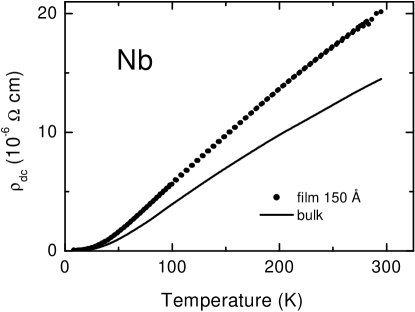
Figure 1: Temperature dependence of phonon part of dc resistivity for thin-film pronin and bulk bulk niobium.

The critical temperature of the film, $T_{c}$ = 8.31 K pronin , is also somewhat below the bulk value (9.3 K), although for films of this thickness, it is rather high greene . The influence of the film thickness on the properties of thin films in the normal and superconducting states is certainly beyond the scope of this work. For detail discussions on this topic we refer to Ref. andreone and references therein. Here we just emphasize that the deviations of all the parameters for the film measured in Ref. pronin from the bulk values are within $\pm 10\%$, thus the investigated film can pretty accurately represent the bulk properties.

From the theoretical point of view, these small differences between the film and bulk properties can be understood, for instance, in terms of a simple approach developed by Testardi and Matteiss testardi . This approach introduces smearing of the first-principles calculated band structure of metals due to the lifetime effects, which are certainly very essential in thin films, and allows to calculate the density of states $N(0)$ and the plasma frequency as function of the phonon ($\rho_{ph}$) and the residual ($\rho_{0}$) resistivity. Although the Testardi-Matteiss approach is oversimplified, it gives the right direction of the change in the film properties compared to the bulk.

For calculation of the frequency dependent conductivity of Nb, we have used the formulas, obtained firstly by Nam nam . Here we present them in a shape convenient for numerical computations:

$$\sigma(\omega)=\frac{\omega_{pl}^{2}}{4\pi i\omega}\cdot\{\int_{0}^{\omega/2}d\omega^{\prime}[f(\omega^{\prime})-f(\omega^{\prime}-\omega)]$$

$$\times\{\frac{1+n(\omega-\omega^{\prime})n(\omega^{\prime})-a(\omega-\omega^{\prime})a(\omega^{\prime})}{\varepsilon(\omega-\omega^{\prime})+\varepsilon(\omega^{\prime})+2i\gamma_{imp}}$$

$$-\frac{1-n(\omega-\omega^{\prime})n^{*}(\omega^{\prime})+a(\omega-\omega^{\prime})a^{*}(\omega^{\prime})}{\varepsilon(\omega-\omega^{\prime})-\varepsilon^{*}(\omega^{\prime})+2i\gamma_{imp}}\}$$

$$+\int_{0}^{\infty}d\omega^{\prime}[f(\omega^{\prime})-f(\omega^{\prime}+\omega)]$$

$$\times\{\frac{1-n(\omega+\omega^{\prime})n(\omega^{\prime})-a(\omega+\omega^{\prime})a(\omega^{\prime})}{\varepsilon(\omega+\omega^{\prime})+\varepsilon(\omega^{\prime})+2i\gamma_{imp}}$$

$$-\frac{1+n(\omega+\omega^{\prime})n^{*}(\omega^{\prime})+a(\omega+\omega^{\prime})a^{*}(\omega^{\prime})}{\varepsilon(\omega+\omega^{\prime})-\varepsilon^{*}(\omega^{\prime})+2i\gamma_{imp}}\}$$

$$-\int_{0}^{\infty}d\omega^{\prime}\tanh(\frac{\omega+\omega^{\prime}}{2T})$$

$$\times Re\frac{1-n(\omega+\omega^{\prime})n(\omega^{\prime})-a(\omega+\omega^{\prime})a(\omega^{\prime})}{\varepsilon(\omega+\omega^{\prime})+\varepsilon(\omega^{\prime})+2i\gamma_{imp}}$$

$$-\int_{0}^{\omega/2}d\omega^{\prime}\tanh(\frac{\omega-\omega^{\prime}}{2T})$$

$$\times Re\frac{1-n(\omega-\omega^{\prime})n^{*}(\omega^{\prime})+a(\omega-\omega^{\prime})a^{*}(\omega^{\prime})}{\varepsilon(\omega-\omega^{\prime})-\varepsilon^{*}(\omega^{\prime})+2i\gamma_{imp}}\},$$ (5)

where $f$ is the Fermi distribution and

$$\varepsilon(\omega)=Z(\omega)\sqrt{\omega^{2}-\Delta^{2}(\omega)},$$

$$n(\omega)=\frac{\omega}{\sqrt{\omega^{2}-\Delta^{2}(\omega)}},$$

$$a(\omega)=\frac{\Delta}{\sqrt{\omega^{2}-\Delta^{2}(\omega)}}.$$ (6)

The renormalization function $Z(\omega)$ and the energy gap $\Delta(\omega)$ have been calculated from the Eliashberg equation eliash , which has a well-known form, and we do not reproduce it here. In our calculations, we used the Eliashberg spectral function $\alpha^{2}F(\omega)$ obtained from the first-principles calculations in Ref. savrasov .

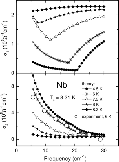
Figure 2: Frequency dependence of the real (upper panel) and imaginary (bottom panel) parts of the complex conductivity of Nb, as calculated from the first principles. Compare to Fig. 4 of Ref. pronin . As an example, we replot the experimental $\sigma_{2}(\omega)$ data from this figure at T = 6 K.

In order to match to the experimentally measured critical temperature of the film, we had to slightly increase the Coulomb pseudopotential $\mu^{*}$ in the Eliashberg equation, in comparison with the bulk value. As films are usually more disordered than bulk samples, and as the disorder is known to increase the value of $\mu^{*}$, this increasing seems to be well grounded sadovskii . Due to the reasons discussed above, while computing the Eq. Far-infrared electrodynamics of superconducting Nb: comparison of theory and experiment, the plasma frequency has also been slightly changed from its bulk value of 9.47 eV to 9.2 eV.

The real and imaginary parts of the complex conductivity, as obtained from our calculations, are shown in Fig. 2 for several temperatures below $T_{c}$. At each temperature, the calculations have been made for 20 - 30 frequency points in the interval from 5 to 30 cm^-1. As temperature goes down, the energy gap clearly develops in the $\sigma_{1}(\omega)$ spectra, $\sigma_{2}(\omega)$ demonstrating a characteristic $1/\omega$-divergency at $\omega\rightarrow 0$.

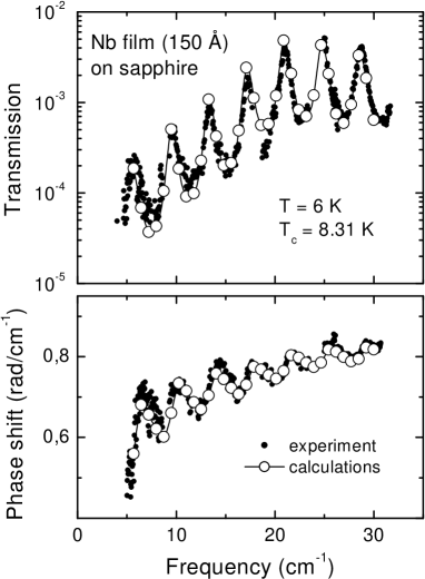
Figure 3: Examples of the transmission and phase shift spectra of a 150-Å-thick Nb film on sapphire substrate. Open symbols - spectra, calculated from the first principles. Solid symbols - experimental data from Ref. pronin .

To compare our computations with the raw experimental data, we calculate the transmission and the phase shift spectra of a Nb film on sapphire substrate (as has been measured experimentally in Ref. pronin ). For these calculations, the optical parameters of the substrate and the thicknesses of the film and of the substrate have been taken from the same reference. The calculations were performed at all temperatures where the experimental data were available. An example of these calculations together with the experimental data are shown in Fig. 3 for $T=6$ K. Clearly, the computed spectra beautifully describe row experimental results.

In Fig. 2, as large open symbols, we show $\sigma_{2}$ data, calculated in Ref. pronin from the experimentally measured transmission and phase shift spectra for $T=6$ K. Our first-principles calculations fit these experimental points very well, while the weak-coupling calculations have been shown to significantly deviate from the experimental values, especially at the lowest frequencies (Fig. 5 of Ref. pronin ). Thus, the effect of strong coupling is clearly seen in the frequency-dependent conductivity in Nb.

We should note, that at the lowest temperatures and low frequencies, the real part of the complex conductivity, calculated in Ref. pronin from the measured transmission and phase shift spectra, does not coincide with our first-principles calculations. We suggest this deviation is caused by the difficulties in solving the inverse task - calculation of $\sigma_{1}(\omega)$ and $\sigma_{2}(\omega)$ from transmission and phase shift. At the lowest temperatures and at frequencies below the gap, the imaginary part of conductivity is much large than the real part. Consequently, the experimentally measured dynamic response (transmission and phase shift in our case) is mainly determined by $\sigma_{2}(\omega)$, while $\sigma_{1}(\omega)$ has quite a minor influence on experimental spectra. That causes large error bars in determination of $\sigma_{1}(\omega)$ from experimental data.

Since the relaxation rate (which can be determined from Eqs. 1 - 2) is much larger than the gap value, or, in other words, the mean free path is smaller than the coherence length, the film is in the dirty limit and the following expression for the penetration depth is valid:

$$\lambda^{-2}(T)=\sigma_{n}\cdot 2\pi Im\int^{\infty}_{0}\frac{\Delta^{2}(\omega)\tanh(\omega/2T)d\omega}{\omega^{2}-\Delta^{2}(\omega)},$$ (7)

where $\sigma_{n}$ is the normal state conductivity:

$$\sigma_{n}=\frac{\omega_{pl}^{2}}{4\pi\gamma_{imp}}.$$ (8)

For $T=4$K, that gives $\lambda=880$ Å, in a good agreement with the experimental result, $\lambda^{exp}=900$ Åpronin .

To make better comparison with the experimental results of Ref. pronin , we now compute the London penetration depth. By the London penetration depth we mean the penetration depth that would be observed in our superconductor, if it were in the clean limit. For this goal, we shall put $\gamma_{imp}$ = 0 in Eqs. Far-infrared electrodynamics of superconducting Nb: comparison of theory and experiment, what gives:

$$\lambda^{-2}_{L}=\frac{\omega_{pl}^{2}}{2\pi}\cdot Re\int_{0}^{\infty}\frac{\Delta^{2}(\omega)\tanh(\omega/2T)d\omega}{(\omega^{2}-\Delta^{2}(\omega))^{3/2}\cdot ReZ(\omega)}$$ (9)

For T = 4 K we obtain $\lambda_{L}$ = 354 Å, again in a perfect agreement with the experimental result, $\lambda_{L}^{exp}$ = 350 Åpronin .

In conclusion, we have demonstrated that the row experimental data on the frequency dependent conductivity of a thin Nb film, obtained in Ref. pronin , can be accurately described by the first-principles calculations made for bulk Nb with just a small ($\pm 10\%$) varying of such parameters as the plasma frequency and the Coulomb pseudopotential. These deviations are most likely connected to the disordered nature of films, and can be understood in terms of the a simple theoretical approach testardi . No Josephson junctions inside the sample are needed to be considered to describe the experimental findings. For the first time, in our knowledge, the first-principles calculations of the complex conductivity of a superconductor, have been successfully compared with the experimentally measured data in the frequency region around the superconducting gap.

We are very grateful to many people for fruitful discussions, especially to O. Dolgov. This work has been partially supported by RFBR (grants Nos. 01-02-16719 and 03-02-16252), by the Program of the Presidium of RAS ”Macroscopic Quantum Mechanics”, and by the Program of the Physical Science Division of RAS ”Strongly correlated electrons”. E.G.M. is grateful to Prof. J.J.M. Braat for the kind hospitality during the visit to the TU Delft, where a part of this work has been done.

References

- (1) M. Tinkham, Introduction to Supercondictivity (McGraw-Hill, New York,1996).
- (2) L.H. Palmer and M. Tinkham, Phys. Rev. 165, 588 (1968); R.R. Joyce and P.L.Richards, Phys. Rev. Lett. 24, 1007 (1970); B. Farnworth and T. Timusk, Phys. Rev. B 10, 8799 (1974).
- (3) P. L. Richards and M. Tinkham, Phys. Rev. 119, 575 (1960).
- (4) S. M. Anlage, D.-H. Wu, J. Mao, S. N. Mao, X. X. Xi, T. Venkatesan, J. L. Peng, and R. L. Greene, Phys. Rev. B 50, 523 (1994)
- (5) O. Klein, E. J. Nicol, K. Holczer, and G. Grüner, Phys. Rev. B 50, 6307 (1994)
- (6) F. Marsiglio, J.P. Carbotte, R. Akis, D. Achkir, and M. Porier, Phys. Rev. B 50, 7203 (1994).
- (7) G.M. Eliashberg, Sov. Phys. JETP 11, 696 (1960).
- (8) G.B. Arnold, J. Zasadzinski, J.W. Osmun, and E.L. Wolf, J. Low Temp. Phys. 40, 225 (1982).
- (9) M.C. Nuss, K.W. Goossen, J.P. Gordon, P.M. Mankiewich, M.L. O’Malley, and M. Bhushan , J. Appl. Phys. 70, 2238 (1991).
- (10) A.V. Pronin, M. Dressel, A. Pimenov, A. Loidl, I.V. Roshchin, L.H. Greene, Phys. Rev. B 57, 14416 (1998).
- (11) J. Halbritter, Phys. Rev. B 60, 12505 (1999).
- (12) S.Y. Savrasov and D.Y. Savrasov, Phys. Rev. B 54, 16487 (1996).
- (13) E.G. Maksimov, Phycics Uspekhi 43, 965 (2000).
- (14) See Fig. 3(d) of Ref. savrasov,
- (15) The absolute values for the film dc resistivity are shown in Fig. 1 of Ref. pronin, . The residual resistivity ratio is equal to 6.5, demonstrating high quality of the film.
- (16) Metals: Electronic Transport Phenomena, edited by K.-H. Hellwege and O. Madelung, Landolt-Börnstein, New Series, Group III, Vol. 15, Pt. a (Springer-Verlag, Berlin, 1982)
- (17) L.H. Greene, J.F. Dorsten, I.V. Roshchin, A.C. Abeyta, T.A. Tanzer, G. Kuchler, W.L. Feldmann, and P.W. Bohn, Czech. J. Phys. 46, Suppl. 6, 3115 (1996).
- (18) A. Andreone, A. Cassinese, M. Iavarone, R. Vaglio, I.I. Kulik and V. Palmieri, Phys. Rev. B 52, 4473 (1995).
- (19) L.R. Testardi and L.F. Mattheiss, Phys. Rev. Lett. 41, 1612 (1978).
- (20) S.B. Nam, Phys. Rev. 156, 470 (1967).
- (21) M.V. Sadovskii Phys. Rep. 282, 225 (1997).