A Finite-Size Scaling Study of a Model of Globular Proteins

Abstract

Grand canonical Monte Carlo simulations are used to explore the metastable fluid-fluid coexistence curve of the modified Lennard-Jones model of globular proteins of ten Wolde and Frenkel (Science, 277, 1975 (1997)). Using both mixed-field finite-size scaling and histogram reweighting methods, the joint distribution of density and energy fluctuations is analyzed at coexistence to accurately determine the critical-point parameters. The subcritical coexistence region is explored using the recently developed hyper-parallel tempering Monte Carlo simulation method along with histogram reweighting to obtain the density distributions. The phase diagram for the metastable fluid-fluid coexistence curve is calculated in close proximity to the critical point, a region previously unattained by simulation.

I Introduction

Many pathological diseases, including sickle cell anemia kn:Galkin and genetic cataracts kn:cat , are known to be caused by the crystallization of certain globular proteins. The importance of proteins is further exemplified by recent advances in genome sequencing, revealing that as much as ninety-eight percent of DNA may be involved in the regulation of their production. Exploring protein structure and activities (proteomics) is a growing research field and should help in our understanding of health and disease on a molecular basis kn:web . Advances in decoding genomes, however, have far and away surpassed those in the determination of protein structure. The growth of high quality protein crystals from solution is important in determining structure and is known to depend sensitively on the initial conditions of the solution. Unfortunately, knowledge of the initial conditions necessary for optimal crystallization has not come easily kn:mcpherson .

Significant progress in understanding the relationship of the initial conditions to the crystal nucleation rates for globular proteins has been made in recent years. It was demonstrated in the theoretical work by Gast, Hall, and Russel kn:gast that the characteristics of the phase diagram of colloids depend sensitively on the range of attraction between the colloidal particles. It was found that for a colloid-colloid attractive interaction of very short range (less than some thirty percent of the colloidal diameter), there are stable fluid and crystal phases and a metastable fluid-fluid phase located below the liquidus line. Other studies kn:other have found similar results. This has also been demonstrated in both experiment kn:ilett and simulation kn:hagen . Rosenbaum, Zamora, and Zukoski kn:rosenbaum linked the experimental observations of George and Wilson kn:wilson with those of colloids. They found that the narrow range in the second virial coefficient for which globular proteins crystallize map onto an effective temperature range for colloidal systems. The phase diagrams of the two systems were analogous. ten Wolde and Frenkel kn:tenwolde then calculated the phase diagram and nucleation rate for a modified Lennard-Jones model of globular proteins, whose range of attractive interaction was small compared with the protein diameter. In this seminal work they showed that the nucleation rate increased by many orders of magnitude in the vicinity of the critical point, suggesting a direct route to effective crystallization. Therefore, accurate knowledge of the region around the critical point provides important information regarding crystallization.

ten Wolde and Frankel  kn:tenwolde studied a modified Lennard-Jones (MLJ) pairwise interaction model given by

$$\large{V(r)}=\left\{\begin{array}[]{cl}\infty,&\mbox{$r<\sigma$}\\ \frac{4\epsilon}{\alpha^{2}}(\frac{1}{[(r/\sigma)^{2}-1]^{6}}-\frac{\alpha}{[(r/\sigma)^{2}-1]^{3}})&\mbox{$r\geq\sigma$}.\end{array}\right.$$ (1)

V(r) is shown in Fig. 1, where $\sigma$ denotes the hard-core diameter of the particles, r is the interparticle distance, and $\epsilon$ is the well depth. The width of the attractive well can be adjusted by varying the parameter $\alpha$; it was tuned in such a way that the so-called stickiness parameter $\tau$ kn:rosenbaum was equal to that produced by the hard-core Yukawa kn:hagen potential for $k=7\sigma^{-1}$ at the metastable liquid-vapor critical point, where $k^{-1}$ is a measure of the range of the attractive part of the potential. In the Yukawa model, the phase diagram for $k=7\sigma^{-1}$ was found to be equivalent to that of globular proteins and maps onto those determined experimentally kn:rosenbaum . An advantage of the MLJ potential is that it lends itself naturally to both Monte Carlo and molecular dynamic simulations. Of particular interest both theoretically kn:tenwolde ; kn:oxtoby ; kn:hagen and experimentally kn:exp1 ; kn:exp2 ; kn:exp3 is the metastable fluid-fluid curve of the phase diagram, for reasons noted above. ten Wolde and Frenkel kn:tenwolde determined the phase diagram for the above model using the Gibbs ensemble Monte Carlo (GEMC) method kn:gibbs where two coexisting phases are separated into two physically detached but thermodynamically connected boxes, the volumes of which are allowed to fluctuate under constant pressure. In the neighborhood of the critical point, however, GEMC cannot be relied upon to provide accurate estimates of the coexistence curve parameters kn:reasons ; kn:reasons2 ; kn:reasons3 . This is evident by considering the metastable region of the phase diagram kn:tenwolde . The error bars in the data points grow larger as the critical point is approached; there are no data points in the immediate vicinity of the critical point. The purpose of this paper, then, is to accurately determine the critical point of the phase diagram of ten Wolde and Frenkel using finite size scaling techniques adapted for simple fluids by Bruce and Wilding and to accurately determine the corresponding subcritical region using the hyper-parallel tempering method.

Figure 1: The potential in Eq. (1) is shown as the solid line. For comparison, the traditional Lennard-Jones potential is shown as the dashed line. The width of the MLJ was chosen so as to agree with the phase diagrams of experimentally determined globular proteins.

II Model

II.1 Theory

To study the critical region of the phase diagram, we use the Bruce and Wilding kn:wilding finite-size scaling method, along with histogram-reweighting kn:swendsen techniques, in conjunction with grand canonical Monte Carlo (GCMC) simulations kn:liquids . We write the reduced chemical potential as $\hat{\mu}=\mu/(k_{B}T)$ and the reduced well depth as $\omega=\epsilon/(k_{B}T)$, with T the temperature of the system. In what follows, we denote $\hat{\mu}$ as $\mu$ for simplicity. The critical point is identified by the critical values of the reduced chemical potential $\mu_{c}$ and well depth $\omega_{c}$. The relevant scaling fields comprise linear combinations of $\mu$ and $\omega$:

$$\tau=\omega_{c}-\omega+s(\mu-\mu_{c})$$ (2)

$$h=\mu-\mu_{c}+r(\omega_{c}-\omega),$$ (3)

with $\tau$ and h the thermal and ordering scaling fields, respectively. The parameters r and s are system-specific parameters, controlling the degree of mixing, and vanish identically when the Ising symmetry is present. Conjugate to these two fields are the scaling operators

$$\mathcal{M}=\frac{1}{1-sr}\>[\rho-su]$$ (4)

$$\mathcal{E}=\frac{1}{1-sr}\>[u-r\rho],$$ (5)

with $\mathcal{M}$ and $\mathcal{E}$ the ordering and energy-like operators, respectively. The (dimensionless) number density and energy density are defined by $\rho=L^{-d}N\sigma^{d}$ and by $u=U/(V\epsilon)$, respectively, with U the total energy of the system, $V=L^{d}$  the volume of the system, and $\epsilon$ the well depth of the potential energy.

We make the usual finite-size scaling ansatz kn:wilding :

$$P_{L}(\mathcal{M},\mathcal{E})\simeq\tilde{P}_{\mathcal{M},\mathcal{E}}(\Lambda_{\mathcal{M}}^{\dagger}\;\delta{\mathcal{M}},\Lambda_{\mathcal{E}}^{\dagger}\;\delta{\mathcal{E}}),$$ (6)

where

$$\Lambda_{\mathcal{E}}=a_{\mathcal{E}}L^{1/\nu},\,\Lambda_{\mathcal{M}}=a_{\mathcal{M}}L^{d-\beta\nu},\,\Lambda_{\mathcal{M}}\Lambda_{\mathcal{M}}^{\dagger}=\,\Lambda_{\mathcal{E}}\Lambda_{\mathcal{E}}^{\dagger}\,=L^{d},$$ (7)

and

$$\delta{\mathcal{M}}=\mathcal{M}-\langle\mathcal{M}\rangle_{c}\;\;\delta{\mathcal{E}}=\mathcal{E}-\langle\mathcal{E}\rangle_{c},$$ (8)

where the parameters $a_{\mathcal{M}}$ and $a_{\mathcal{E}}$ are non-universal scaling factors, $\beta$ and $\nu$ are the critical exponents for the coexistence curve and the correlation length kn:stanley , respectively, and the subscript c in the above equations denotes that the averages are to be taken at criticality. From our simulations using GCMC, we obtain the joint probability distribution of $\rho$ and u at a particular point in parameter space of inverse temperature (T) $\beta$ and reduced chemical potential $\mu$ from which we obtain the joint probability distribution of mixed operators via

$$P_{L}(\mathcal{M},\mathcal{E})=(1-sr)\,P_{L}(\rho,u).$$ (9)

Integrating out the energy-like dependence from the latter distribution gives

$$P_{L}(\mathcal{M})=\int d\mathcal{E}\,P_{L}(\mathcal{M},\mathcal{E}).$$ (10)

Using the fact  kn:exper1 ; kn:exper2 ; kn:theory1 ; kn:theory2 ; kn:sim ; kn:sim2 that the critical behavior of this distribution is in the same universality class as the Ising model, we match the above probability distribution to that of the universal fixed point function

$$\tilde{P}^{*}_{\mathcal{M}}(x)=\int\tilde{P}^{*}_{\mathcal{M},\mathcal{E}}(x,y)\,dy,$$ (11)

which is known from an independent study kn:lattice . The critical point of the fluid can thus be estimated by tuning the temperature T, chemical potential $\mu$, and field-mixing parameter s such that $P_{L}(\mathcal{M})$ collapses onto $\tilde{P}^{*}_{\mathcal{M}}(x)$.

To save computer-time and to facilitate the matching process, we employ histogram-reweighting kn:swendsen in lieu of performing tedious simulations. Once the joint probability distribution at a particular point in parameter space $(\beta,\mu)$ is obtained in one simulation run, information around its neighboring points in parameter space $(\beta^{\prime},\mu^{\prime})$ is extracted using

$$P^{(\beta^{\prime},\mu^{\prime})}_{L}(\rho,u)=$$

$$\frac{\exp[(\mu^{\prime}-\mu)\rho V-(\beta^{\prime}-\beta)uV]P^{(\beta,\mu)}_{L}(\rho,u)}{\sum\exp[(\mu^{\prime}-\mu)\rho V-(\beta^{\prime}-\beta)uV]P^{(\beta,\mu)}_{L}(\rho,u)}.$$ (12)

Histogram-reweighting provides an accurate determination of the new probability distribution and is well suited for Monte Carlo studies. Its limitations are discussed elsewhere kn:limit .

In the subcritical region, we employ hyper-parallel tempering kn:yan Monte Carlo (HPTMC) to sample the joint probability distribution. Below the critical point, density fluctuations are no longer large enough for the joint probability distribution to be accessible by standard Monte Carlo simulations. Thus, a free energy barrier exists below $T_{c}$ which needs to be overcome if one is to sample both coexisting phases. HPTMC allows one to effectively tunnel through this barrier by swapping particle configurations between different simulations (replicas) at different state points. Other techniques kn:berg sample this region by artificially lowering this barrier.

In the grand canonical ensemble, the partition function can be written as

$$Z=\sum_{x}\Omega(x)exp[-\beta U(x)+\mu N(x)],$$ (13)

where x denotes the state of the system, $\Omega(x)$ is the density of states, $U(x)$ is the total energy of state x, and $N(x)$ is the number of particles in state x, and all other variables are defined as above. In accord with practice kn:yan , we consider a composite ensemble consisting of M non-interacting replicas, each at a different set of state points. The partition function of the composite ensemble is specified by

$$Z_{c}=\prod_{i=1}^{M}Z_{i},$$ (14)

where the complete state of the composite ensemble is given by

$$\textbf{x}=(x_{1},x_{2},...,x_{M}),$$ (15)

with $x_{i}$ denoting the state of the $i^{th}$ replica. The unnormalized probability density of the composite state x is given by

$$p(\textbf{x})=\prod_{i=1}^{M}exp[-\beta U(x_{i})+\mu N(x_{i})].$$ (16)

To sample configurations from the composite ensemble, a Markov chain is constructed to generate configurations according to the limiting function in Eq. (16). In the Markov chain, two types of trial moves are employed: 1) within each replica, insertion/deletion trial moves are attempted according to standard Monte Carlo as adapted for use in the grand canonical ensemble kn:liquids , and 2) Configuration swaps are attempted between pairs of replicas i and i+1 such that

$$x_{i}^{new}=x_{i+1}^{old},\;\;\;x_{i+1}^{new}=x_{i}^{old}.$$ (17)

To enforce a detailed-balance condition, the pair of replicas that are attempted to be swapped are chosen at random, and the trial swap is accepted with the probability

$$p_{acc}(x_{i}\leftrightarrow x_{i+1})=min[1,exp(\Delta\beta\Delta U-\Delta\mu\Delta N)],$$ (18)

where $\Delta\beta=\beta_{i+1}-\beta_{i}$, $\Delta U=U(x_{i+1})-U(x_{i})$, $\Delta\mu=\mu_{i+1}-\mu_{i}$, and $\Delta N=N(x_{i+1})-N(x_{i})$. Once joint probability distributions are obtained in this way, histogram reweighting is applied to obtain coexistence according to Eq. (12) and an ”equal-weight” kn:hill construction:

$$\int_{0}^{\langle\rho\rangle}P_{L}^{(\beta^{\prime}\mu^{\prime})}(\rho)=0.5.$$ (19)

It should be recognized that the average density $\langle\rho\rangle$ in the upper limit of the integral in Eq. (19) is itself a function of temperature and chemical potential and can therefore be obtained from the first moment of the reweighted histogram.

II.2 Computational Details

We studied a system of N particles contained in a three-dimensional, periodic cubic simulation cell having a volume $V=L^{d}$. Two particles separated by a distance r interact via the modified Lennard-Jones (MLJ) pair potential given in Eq. (1), where $\epsilon$ and $\sigma$ denote the energy and length scales, respectively. The total energy, U, is obtained by summing over all distinct pairs of particles. We employ a truncated, unshifted version of Eq. (1) using a cutoff radius $r_{c}=2.0\,\sigma$, in accord kn:foot with ten Wolde and Frenkel. The simulations were performed on system sizes of $L=6\,\sigma,7\,\sigma,8\,\sigma$, and $10\,\sigma$, implemented using the Metropolis Monte Carlo method as adapted for use in the grand canonical ensemble kn:liquids with a constant volume $L^{d}$, inverse temperature (T) $\beta$, and reduced chemical potential $\mu$. The thermodynamic potential needed is actually $\mu^{*}=\mu-3\;ln[\Lambda/\sigma]$ (where $\Lambda$ is the thermal deBroglie wavelength) kn:liquids . As in other implementations kn:masha , only particle insertion and deletion steps were employed, particle displacements being realized within the cell from a succession of such steps. In our simulations, equilibrium times used were approximately two million steps and production runs ranged from 500 million steps for the smaller system sizes to one billion steps for the higher system sizes. Such a high number of steps was needed in order to obtain smooth distributions at the low temperatures we are studying. We emphasize that the true equilibrium state of the system is that of fluid and solid coexistence. GCMC, however, is limited to ’low’ densities and, thus, the solid region of the phase diagram is unaccessible.

Using a previous estimate of the critical temperature kn:thesis for this model, we first attempted to locate the critical point by tuning the reduced chemical potential $\mu^{*}$ until the density distribution exhibited a double peaked structure. Once obtained, longer runs were performed to accumulate better statistics. To obtain two-phase coexistence and appropriate values of the field-mixing parameter s, we adopted the criterion kn:wilding that the order distribution $P_{L}(\mathcal{M})=\int d\mathcal{E}\,P_{L}(\mathcal{M},\mathcal{E})$ be symmetric in $\mathcal{M\,-\,}\langle\mathcal{M}\rangle$. This criterion is the counterpart of the coexistence symmetry condition for the Ising model magnetization distribution. Having obtained in this manner a two-phase distribution near the critical point, we then matched the order-operator distribution $P_{L}(\mathcal{M})$ to that of the universal fixed point distribution $\tilde{P}^{*}_{\mathcal{M}}(x)$. Employing histogram-reweighting, we tuned the chemical potential $\mu^{*}$, temperature T, and mixed-field parameter s until our distribution $P_{L}(\mathcal{M})$ collapsed onto that of the fixed point distribution. Once that was attained, we then attempted to match $P_{L}(\mathcal{E})$ to the corresponding energy-like fixed point distribution $\tilde{P}^{*}_{\mathcal{E}}(y)$ by tuning the field-mixing parameter r. This procedure was repeated for the various system sizes studied.

In the subcritical region, we used six replicas for the $L=7\,\sigma$ system to obtain joint probability distributions. Small runs of approximately five million steps were first performed to optimize the choice of $\mu^{*}$ for each replica. At low temperatures, $\mu^{*}$ was chosen so that the density distribution was biased toward a high-density peak; conversely, at high temperatures, $\mu^{*}$ was chosen so that low-density peaks were favored. Such a choice of $\mu^{*}$ allowed high-density configurations to be ”melted” when passed to high temperatures, allowing for a fuller exploration of configuration space kn:yan . Also, we chose these values so that a high swap frequency between replicas was realized. On average, replicas were swapped twenty-five percent of the time. Once these criteria were satisfied, Monte Carlo runs were extended to approximately 150 million steps to acquire good statistics. Histogram-reweighting was then applied to the resulting joint probability distributions to obtain coexistence in the subcritical region in accordance with Eq. (12) and Eq. (19).

III Results

The resulting density distributions obtained in the prescribed manner at the size-dependent critical point $T_{c}(L)$ and $\mu^{*}_{c}(L)$ are shown in Fig. 2. As is evident, the distributions become narrower with increasing system size $L$, approaching the limiting form of the fixed point distribution $\tilde{P}^{*}_{\mathcal{M}}(x)$. The corresponding energy-density distributions are shown in Fig. 3.

Both distributions show an asymmetry, due to field-mixing effects, with that of $P_{L}(u)$ being much more pronounced. These effects die off with increasing L, so that the limiting forms of both $P_{L}(\rho)$ and $P_{L}(u)$ match the fixed point distribution $\tilde{P}^{*}_{\mathcal{M}}(x)$. As noted, this limiting form is easily recognizable for the density distributions. However, the limiting form of the energy density distributions does not follow this pattern. This difference is attributable to the coupling that occurs for asymmetric systems between the ordering operator and energy-like operator fluctuations. Those of $\mathcal{M}$ dominate at large L, while those in $\mathcal{E}$ do not kn:wilding_fluctuate ; kn:wilding_finite . Thus, a ’background’ effect perturbs the energy-density distributions.

Figure 2: Density distributions at $T_{c}(L)$ and $\mu^{*}_{c}(L)$ for the system sizes $L=6\sigma,8\sigma,$ and $10\sigma$. For clarity, the distribution corresponding to the $L=7$ system size is not shown.

Figure 3: Energy distributions at $T_{c}(L)$ and $\mu^{*}_{c}(L)$ for the system sizes $L=6\sigma,7\sigma,8\sigma,$ and $10\sigma$.

Our estimates for the fixed point distribution are shown in Fig. 4. As is seen from the figure, the agreement is good for all system sizes studied. This matching alone allows us to accurately determine the critical point $T_{c}(L)$ and $\mu^{*}_{c}(L)$ and to also obtain good estimates of the field-mixing parameter s. Though matching of $P_{L}(\mathcal{E})$ to $\tilde{P}^{*}_{\mathcal{E}}(y)$ should also give good estimates of the critical point, and the field-mixing parameter r, fluctuations in the energy-like operator $\mathcal{E}$ are relatively weak and therefore do not allow for good matching kn:micro . It is unknown presently how to remove this background effect for fluid-systems, though it has been removed for the Ising model kn:micro . Nevertheless, we can still obtain a rough estimate for the field-mixing parameter r by observing that the distributions $P_{L}(\mathcal{E})$ should have a shape similar to $\tilde{P}^{*}_{\mathcal{E}}(y)$. For completeness, we include these curves along with the energy-fixed point function in Fig. 5.

Figure 4: The measured form of the ordering operator distribution $P_{L}(\mathcal{M})$ for the system sizes studied. Shown for comparison is the universal fixed-point ordering operator distribution $\tilde{P}^{*}_{\mathcal{M}}(x)$ (solid line). The data have been expressed in terms of the scaled variable $x=a_{\mathcal{M}}^{-1}L^{\beta/\nu}(\mathcal{M}-\mathcal{M}_{c})$, where $a^{-1}_{\mathcal{M}}$ was chosen such that the distributions have unit variance.

Figure 5: The measured form of the energy-like operator distribution $P_{L}(\mathcal{E})$ for the system sizes studied. Shown for comparison is the universal fixed-point ordering operator distribution $\tilde{P}^{*}_{\mathcal{E}}(y)$ (solid line). The data have been expressed in terms of the scaled variable $y=a_{\mathcal{E}}^{-1}L^{d-1/\nu}(\mathcal{E}-\mathcal{E}_{c})$, where $a^{-1}_{\mathcal{E}}$ was chosen such that the distributions have unit variance. The lines are a guide to the eye.

From estimates of the finite critical-point temperatures $T_{c}(L)$, we can estimate the critical-point for the infinite-volume system. Since contributions to $P_{L}(\mathcal{M})$ from finite values of $\tau$ grow with system size like $\tau L^{1/\nu}$, the matching condition results in a deviation from the true critical point $T_{c}(\infty)$ as

$$T_{c}(\infty)-T_{c}(L)\propto L^{-(\theta+1)/\nu},$$ (20)

where $\theta$ is the universal correction to scaling exponent kn:theta and $\nu$ is the critical exponent for the correlation length kn:stanley . In Fig. 6, we plot the apparent critical temperature $T_{c}(L)$ as a function of $L^{-(\theta+1)/\nu}$. By extrapolating to infinite volume, we arrive at an estimate for the true critical temperature. Similar arguments in accounting for field-mixing effects kn:wilding_fluctuate apply in obtaining the true critical density via

$$\langle\rho\rangle_{c}(L)-\langle\rho\rangle_{c}(\infty)\propto L^{-(d-1/\nu)},$$ (21)

where d is the dimensionality of the system. In Fig. 7, $\langle\rho\rangle_{c}(L)$ is plotted as a function of $L^{-(d-1/\nu)}$ to obtain an estimate of the true critical density. We summarize our findings in Table I.

Figure 6: The apparent reduced critical temperature plotted as a function of $L^{-(\theta+1)/\nu}$, with $\theta=0.54~{}\cite[cite]{\@@bibref{Authors Phrase1YearPhrase2}{kn:theta}{\@@citephrase{(}}{\@@citephrase{)}}}$ and $\nu=0.629$ kn:values . The extrapolation to infinite volume yields the estimate $T_{c}=.4145(5)$.

Table 1: Summary of results for location of the critical point

L	$T_{c}(L)$	$\mu^{*}_{c}(L)$	$\langle\rho\rangle_{c}(L)$	s	r
6	.4120$(3)$	-2.939$(1)$	.312$(2)$	-0.120$(3)$	-0.65$(5)$
7	.4130$(2)$	-2.932$(2)$	.312$(2)$	-0.115$(2)$	-0.65$(5)$
8	.4135$(3)$	-2.930$(2)$	.318$(4)$	-0.110$(1)$	-0.65$(5)$
10	.4136$(6)$	-2.932$(3)$	.315$(5)$	-0.110$(1)$	-0.65$(5)$

Figure 7: The measured average density $\langle\rho\rangle_{c}(L)$ at the L-dependent critical point expressed as a function of $L^{-(d-1)/\nu}$. Extrapolation to infinite volume yields the estimate $\rho_{c}=.3206(4)$.

Figure 8: The coexistence density distributions for the $L=7\,\sigma$ system size for a range of subcritical temperatures, obtained using HPTMC as described in the text.

Table 2: Values of T and $\mu^{*}$ used in HPTMC. Also shown are the reweighted chemical potentials $\mu^{*}_{R}$ used in obtaining the coexisting densities $\rho_{v}$ and $\rho_{l}$.

Replica	$T$	$\mu^{*}$	$\mu^{*}_{R}$	$\rho_{v}$	$\rho_{l}$
1	.400	-3.110	-3.137	.120	.531
2	.404	-3.040	-3.071	.140	.510
3	.406	-3.010	-3.041	.149	.495
4	.409	-2.970	-2.995	.170	.473
5	.4115	-2.947	-2.957	.186	.444
6	.4123	-2.941	-2.946	.192	.441

Using HPTMC, we were able to obtain joint distribution functions corresponding to points in the subcritical region of the phase diagram of ten Wolde and Frenkel. The choices we employed for the values of the temperature T and chemical potential $\mu^{*}$ of each replica are displayed in Table II, along with the coexisting chemical potentials $\mu^{*}_{R}$ and coexisting densities $\rho_{v}$ and $\rho_{l}$, obtained after reweighting. The corresponding density distributions in this region are shown in Fig. 8, where the temperatures are expressed in terms of the infinite-volume critical temperature. It can be seen that for temperatures even as high as $T=.965\,T_{c}$, the system has a vanishingly small probability of visiting a state between the two coexisting phases. This implies, as stated previously, that one cannot expect standard Monte Carlo simulations to obtain these subcritical distributions.

In Fig. 9, we plot the temperatures used in Table II as a function of density, where we have calculated the average densities for each of the two phases from the distributions shown in Fig. 8. These new results are consistent with the earlier results for the metastable coexistence curve of the phase diagram kn:tenwolde and extend much closer to the critical point. We also show our attempt to fit this subcritical density data to a power-law of the form $\rho_{\pm}-\rho_{c}=A\,|T-T_{c}|\>\pm\>B\,|T-T_{c}|^{\beta}$, where $T_{c}$ and $\rho_{c}$ are are our extrapolated values as $L\rightarrow\infty$ and $\beta=.3258~{}\cite[cite]{\@@bibref{Authors Phrase1YearPhrase2}{kn:values}{\@@citephrase{(}}{\@@citephrase{)}}}$ is the Ising exponent. Although the data are in reasonable agreement with this fit, note that we have not accounted for possible finite-size effects, preventing this from being a definitive test. Fig. 10 shows the corresponding chemical potential as a function of temperature, which obeys a linear relationship in this region. Experimental kn:schurt investigations on the bovine lens protein, $\gamma_{II}-crystallin$, have been performed near the critical point. They report values for the critical isothermal compressibility $\gamma=1.21\pm 0.05$ and the critical correlation length $\nu=0.68\pm 0.1$. Both results are compatible to three-dimensional Ising model values.

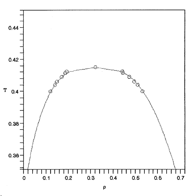
Figure 9: Temperature plotted vs. density, as obtained from HPTMC simulations for the $L=7\,\sigma$ system size shown with the critical point $T_{c}(\infty)$ and the corresponding critical density $\rho_{c}$ as obtained by Eqs. (20) and (21). Also shown (solid line) is a fit to the data, with $\beta=.3258~{}\cite[cite]{\@@bibref{Authors Phrase1YearPhrase2}{kn:values}{\@@citephrase{(}}{\@@citephrase{)}}}$.

Figure 10: The chemical potential $\mu^{*}_{R}$ vs. $T$ for the system size $L=7\,\sigma$ for the coexisting subcritical region obtained using HPTMC as described in the text. Errors do not exceed symbol size.

IV Conclusion

In this work, we have employed mixed-field finite-size scaling techniques and histogram extrapolation methods to obtain accurate estimates for the critical-point parameters of the truncated, unshifted MLJ fluid with $r_{c}=2.0\,\sigma$. Our measurements allow us to pinpoint the critical-point parameters to within high accuracy. A previous estimate put the critical point at $T_{c}=.420$ kn:thesis , slightly higher than our estimate of $T_{c}(\infty)=.4145(5)$. In the near subcritical region, we have explored the phase diagram and obtained data in a region where no prior estimates were available. HPTMC proved to be an efficient means toward this end.

- (1) O. Galkin et al., PNAS 99, 8479 (2002)
- (2) Ajaye Pande et al., PNAS 98, 6116 (2001)
- (3) World Wide Web, U.S. Department of Energy Office of Science, http://www.doegenomes.org
- (4) A. McPherson, Preparation and Analysis of Protein Crystals, (Krieger, Malabar, FL., 1982)
- (5) A. P. Gast, C. K. Hall, and W. B. Russel, J. Colloid Interface Sci., 96, 251 (1983)
- (6) H. N. W. Lekkerkerker et al., Europhys. Lett., 20, 559 (1992); Tejero et al., Phys. Rev. Lett., 73, 752 (1994)
- (7) S. M. Ilett et al., Phys. Rev. E, 51, 1344 (1995)
- (8) M. H. J. Hagen and D. Frenkel, J. Chem. Phys., 101, 4093, (1994)
- (9) D. Rosenbaum, P.C. Zamora, and C.F. Zukoski, Phys. Rev. Lett., 76, 150 (1996)
- (10) A. George and W. Wilson, Acta Cryst. D 50, 361 (1994)
- (11) P. R. ten Wolde and D. Frenkel, Science, 277, 1975 (1997)
- (12) D. W. Oxtoby and V. Talanquer, J. Chem. Phys., 101, 223 (1998)
- (13) C. R. Berland et al., PNAS, 89, 1214 (1992)
- (14) N. Asherie, et al., Phys. Rev. Lett., 77, 4832 (1996)
- (15) M. L. Broide et al., Phys. Rev. E, 53, 6325 (1996)
- (16) A. Z. Panagiotopoulos, Mol. Phys. 61, 813 (1987)
- (17) N. B. Wilding and A. D. Bruce, J. Phys. Condens. Matter 4, 3087 (1992)
- (18) K. K. Mon and K. Binder, J. Chem. Phys. 96, 6989 (1992)
- (19) J. R. Recht and A. Z. Panagiotopoulos, Mol. Phys. 80, 843 (1993)
- (20) N. B. Wilding, Phys. Rev. E, 52, 602 (1995)
- (21) A. M. Ferrenberg and R. H. Swendsen, Phys. Rev. Lett., 61, 2635 (1988)
- (22) M. P. Allen and D. J. Tildesley, Computer Simulations of Liquids, (Clarendon, Oxford, 1990)
- (23) H. Eugene Stanley, Introduction to Phase Transitions and Critical Phenomena, (Oxford University Press, New York 1972)
- (24) M. W. Pestak and M. H. W. Chan, Phys. Rev. B, 30, 274 (1984)
- (25) U. Närger and D. A. Balzarani, Phys. Rev. B 42, 6651 (1990); U. Närger, J. R. de Bruyn, M. Stein, and D. A. Balzarini, ibid. 39, 11 914 (1989)
- (26) J. V. Sengers and J. M. H. Lefelt Sengers, Annu. Rev. Phys. Chem. 37, 189 (1986)
- (27) Q. Zhang and J. P. Badiali, Phys. Rev. Lett. 67, 1598 (1991); Phys. Rev. A 45, 8666 (1992)
- (28) J. F. Nicoll, Phys. Rev. A 24, 2203 (1981)
- (29) A. D. Bruce and N. B. Wilding, Phys. Rev. Lett. 68, 193 (1992)
- (30) M. M. Tsypin and H. W. J. Blöte, Phys. Rev. E, 62, 73 (2000)
- (31) Robert H. Swendsen, Physica A, 194, 53, (1993)
- (32) Qiliang Yan and Juan J. de Pablo, J. Chem. Phys., 111, 9509 (1999)
- (33) Bernd A. Berg and Thomas Neuhaus, Phys. Rev. Lett., 68, 9 (1991)
- (34) T. L. Hill, Thermodynamics of Small systems, (Dover, New York, 1962)
- (35) The potential was shifted in ref. [11].
- (36) J. M. Caillol, J. Chem. Phys., 109, 4885 (1998)
- (37) P. R. ten Wolde, Thesis for Ph.D.
- (38) N. B. Wilding and M. Müller, J. Chem. Phys., 102, 2562 (1995)
- (39) M. Müller and N. B. Wilding, Phys. Rev. E, 51, 2079 (1995)
- (40) A. D. Bruce and N. B. Wilding, Phys. Rev. E, 60, 3748 (1999)
- (41) Jing-Huei Chen, et al., Phys. Rev. Lett., 48, 630 (1982)
- (42) A. M. Ferrenberg and D. P. Landau, Phys. Rev. B, 44, 5081 (1991)
- (43) Peter Schurtenberger et al., Phys. Rev. Lett., 63 2064 (1989); ibid, 71, 3395 (1993)