Extremal Properties of Random Structures

Abstract

The extremal characteristics of random structures, including trees, graphs, and networks, are discussed. A statistical physics approach is employed in which extremal properties are obtained through suitably defined rate equations. A variety of unusual time dependences and system-size dependences for basic extremal properties are obtained.

1 Introduction

The goal of this article is to show that methods of non-equilibrium statistical physics are very useful for analyzing extreme properties of random structures. Extremes are compelling human curiosities — we are naturally drawn to compilations of various pinnacles of endeavor, such as lists of the most beautiful people, the richest people, the most-cited scientists, athletic records, etc guiness . More importantly, extremes often manifest themselves in catastrophes, such as the failure of space shuttles, the breaching of dams in flood conditions, or stock market crashes. The theory of extreme statistics ejg ; jg ; res is a powerful tool for describing the extremes of a set of independent random variables; however, much less is known about extremes of correlated variables cl ; dm ; rcps . Such an understanding is crucial, since complex systems are composed of many subsystems that are highly correlated.

While estimates for the failure probability of a nuclear plant or a space shuttle still involve guesswork, understanding the extremes of certain correlated random variables is a hard science. Below we demonstrate this thesis for various extremal characteristics of geometrical features in basic evolving structures, such as randomly growing trees, graphs, and networks. In each case, the growth process of the structure induces correlations in the variables whose extremes are the focus of this review. We shall illustrate how the statistical physics of classical irreversible processes can be naturally adapted to elucidate both typical and extremal statistics.

We obtain new scaling laws for extreme properties and consequently give new insights for a variety of applications. For example, random trees arise naturally in data storage algorithms hmm ; dek ; ws , an important branch of computer science, and the maximal branch height yields the worst-case performance of data retrieval algorithms. Random trees also describe various non-equilibrium processes, such as irreversible aggregation mvs ; sc and collisions in gases vvd . Random graphs bb ; jlr have numerous applications to computer science and to physical processes such as polymerization pjf . Random growing networks are used to model the distributions of biological genera, word frequencies, and income yule ; simon , the structure of the Internet willinger , the World-Wide Web applics , and social networks sp ; gn .

As a subtext to this review, it is worth mentioning that problems at the interface of statistical physics and computer science have been fruitful and symbiotic. Algorithms and methods developed in one area have found application in the other field; important examples include the Monte Carlo method, simulated annealing, and the Dijkstra algorithm. Statistical physics concepts such as criticality, scaling, universality, and techniques such as replicas have proved useful in diverse interdisciplinary applications such as algorithmic complexity, combinatorial optimization, error correction, compression algorithms, and image restoration; a review of these topics can be found in Refs. mmz ; hn ; mpz ; jb ; fps ; ks .

We will focus on three ubiquitous random structures — trees, graphs, and networks. Random trees (Sec. 2) can be viewed as the space-time diagram of irreversible aggregation with a size-independent merging rate. This connection allows to apply well-known results in aggregation to elucidate the growth of the largest component (the leader) and the number of changes in its identity. The number of lead changes grows quadratically with logarithm of the system size. The time-dependent number of lead changes becomes asymptotically self-similar, following a scaling form in which the scaling variable involves a logarithmic, rather than an algebraic ratio, between the typical size and the system size. Qualitatively similar properties also characterize the smallest component in the system.

Another characteristic of random trees is their height. The corresponding branch height distribution is Poissonian, reflecting the random nature of the merger process that underlies tree growth. The growth of the tree height (the maximal branch height) has an interesting relation to traveling wave propagation. The velocity of this wave yields typical and extremal height statistics as a corollary.

Random graphs (Sec. 3) are also equivalent to an aggregation process in which the merging rate of two components is proportional to the product of their sizes. This system undergoes a gelation transition in which a giant component, that contains a finite fraction of the entire mass in the system, arises. Near this transition, the size distribution of graph components follows a self-similar behavior. Despite the differences with the size distribution of random trees, leadership statistics in these two systems are remarkably robust.

Random networks (Sec. 4) can be grown by adding nodes and attaching the new node to a pre-existing node with a rate that depends on the degree of the target node. A hallmark of such systems is the statement that “the rich get richer”; that is, the more popular nodes tend to remain so. This adage is in keeping with human experience — a person who is rich is likely to stay rich, as evidenced by the continued appearance of the same individuals on lists of wealthiest individuals wealth . We examine whether the rich really get richer in growing networks by studying properties of the nodes with the largest degree. In keeping with analysis of random trees and graphs, we focus on the identity of the most popular node as a function of time, the expected degree of this most popular node, and the number of lead changes in the most popular node as a function of time.

2 Random Trees

Random trees underlie physical processes such as coagulation, collisions in gases vvd , and the fragmentation of solids ho ; km . They are also important in computer science algorithms such as data storage and retrieval hmm ; dek ; bp ; ld ; pn ; mk1 . Different extremal characteristics may be important in different contexts. In aggregation processes, the maximal aggregate size is of interest. In other cases, the maximal or the minimal branch height are of interest. In Lorentz gases, the maximum branch height is related to the largest Lyapunov exponent, while in data storage, extremal heights yield best-case and worst-case algorithm performances.

Figure 1: Random trees. A forest of random growing trees is equivalent to the space-time evolution of irreversible aggregation with a size-independent merging rate. Each branch corresponds to the world line of a cluster. The thickness of each branch is proportional to the size of the cluster. The sizes of the 4 trees are (left to right) 3, 1, 4, 2 and their heights are 2, 0, 3, 1.

Consider a forest of random trees that is generated randomly as follows (Fig. 1). Starting with $N$ single-branch trees, two trees are picked randomly and merged. This process is repeated until a single tree containing all $N$ branches is generated. We treat the merger process dynamically. Let $k$ be the number of trees. The transition $k\to k-1$ occurs with rate $r_{k}$ proportional to the total number of pairs. Choosing $2/N$ as the merger rate for each pair (i.e., $r_{k}=k(k-1)/N$) is convenient as in the thermodynamic limit $N\to\infty$, the normalized density $c=\langle k\rangle/N$ evolves according to $\frac{d}{dt}c=-c^{2}$. Given the initial condition $c(0)=1$, the density is

$$c(t)=\frac{1}{1+t}.$$ (1)

The number of trees is therefore ${\cal N}=\langle k\rangle=N(1+t)^{-1}$. Moreover, conservation of the total number of branches yields the average tree size $m=1+t$. The results are stated in terms of the physical time $t$, but can be easily re-expressed in terms of the intrinsic quantities ${\cal N}$ or $m$.

2.1 Size Statistics

Let $n_{k}(t)$ be the number of trees with $k$ branches at time $t$. The normalized density $c_{k}(t)=n_{k}(t)/N$ evolves according to the Smoluchowski rate equation mvs ; sc ; da

$$\frac{dc_{k}}{dt}=\sum_{i+j=k}c_{i}c_{j}-2cc_{k}$$ (2)

with the monodisperse initial conditions $c_{k}(0)=\delta_{k,1}$. This evolution equation reflects the fact that trees merge randomly, independent of their size. The well-known solution to this equation is

$$c_{k}(t)=\frac{t^{k-1}}{(1+t)^{k+1}}.$$ (3)

Taking the long time limit $t\to\infty$ while keeping the variable $k/t$ fixed, the size distribution approaches the asymptotic form $c_{k}(t)\to t^{-2}e^{-k/t}$. More generally, this can be recast as the scaling form

$$c_{k}(t)\simeq k_{*}^{-2}\Phi(k/k_{*}),$$ (4)

with the scaling function $\Phi(z)=e^{-z}$ and the typical tree size $k_{*}\simeq t$.

2.2 The Leader

Extremal characteristics, such as the size of the largest tree — the leader — and the number of lead changes, follow directly from the size distribution. We focus on the asymptotic time regime, where most of the lead changes occur, and use the scaled size distribution (4). Let $l(t,N)$ be the average size of the leader at time $t$. The basic criterion used to determine the size of the leader is

$$U_{l}(t)\equiv\sum_{j\geq l}n_{j}\simeq Nt^{-1}e^{-l/t}=1.$$ (5)

This simply states that there is one cluster whose size exceeds $l(t,N)$. Solving for the leader size gives

$$l(t,N)\simeq t\,\ln\frac{N}{t}.$$ (6)

This expression holds in the asymptotic time regime $t\gg 1$. For short times the leader size grows logarithmically with system size $l(t\approx 1)\sim\ln N$. Finally, at times of the order $N$, the leader becomes of the order of the system size. The final leader, that is, the ultimate winner, emerges on a time scale of the order $N$. This is consistent with the fact that the average “final” time for a single tree to remain in the system $t_{f}$, is given by $t_{f}=N-1$ as follows from ${\cal N}=1$.

We now consider the quantity $L(t,N)$, defined as the average number of lead changes during the time interval $(0,t)$. Lead changes occur when two trees (neither of which is the leader) merge and overtake the leader. The flux of probability to surpass the leader is simply the rate of change of the cumulative distribution. Thus $\frac{d}{dt}L(t,N)=\frac{\partial}{\partial t}U_{k}\big{|}_{k=l}$. Using $U_{l}=1$ yields $\frac{d}{dt}L(t,N)\simeq lt^{-2}\simeq t^{-1}\ln\frac{N}{t}$. Therefore, the time-dependent number of lead changes is bk

$$L(t,N)\simeq\ln t\ln N-\frac{1}{2}(\ln t)^{2},$$ (7)

which can be recast in the self-similar form

$$L(t,N)\simeq(\ln N)^{2}\,F(x),\qquad x=\frac{\ln t}{\ln N},$$ (8)

with the quadratic scaling function $F(x)=x-\frac{1}{2}x^{2}$. Notice the unusual scaling variable — a ratio of logarithms — in contrast to the ordinary scaling variable $z=k/k_{*}$ underlying the size distribution (4). The scaling variable still involves the typical size, $x=\ln k_{*}/\ln N$. Note also that the leader size (6) can be expressed in terms of the same scaling variable $l(t,N)\simeq t\ln N\,f(x)$ with $f(x)=\frac{d}{dx}F(x)=1-x$. Numerical simulations confirm this scaling behavior bk . However, the convergence to these asymptotics is slow due to the logarithmic functional dependences on the system size and time.

The total number of lead changes $L(N)$ as a function of system size $N$ follows from the time dependent behavior (7). The eventual winner emerges at time of order $N$. Using $L(N)\cong L(t\propto N,N)$ we obtain

$$L(N)\simeq A(\ln N)^{2}\,$$ (9)

with $A=F(1)=1/2$ (see Fig. 2). The correction to this leading asymptotic behavior is of the order $\ln N$. The logarithmic dependence implies that lead changes are relatively infrequent.

Both the size of the leader and the number of lead changes grow logarithmically in the early time regime, $l(t\approx 1,N)\propto L(t\approx 1,N)\propto\ln N$. The first relation implies that initially the leader size predominantly grows in increments of one and every leader is a new leader. When $t\gg 1$, the size of the leader greatly exceeds the number of lead changes as the increments of the leader size grow roughly linearly with time.

Figure 2: The total number of lead changes $L(N)$ versus the system size $N$. The simulation data represents an average over $10^{4}$ independent realizations of the random tree generation process with $N$ up to $10^{8}$.

The distribution of the number of lead changes $P_{n}(t,N)$, i.e., the probability that $n$ lead changes occur by time $t$, can be determined by noting that lead changes occur by a random process in which the average flux of probability to surpass the leader is $\frac{d}{dt}L$. Hence, the probability distribution obeys $\frac{d}{dt}P_{n}=(\frac{d}{dt}L)\,[P_{n-1}-P_{n}]$ with the initial condition $P_{n}(0,N)=\delta_{n,0}$. Therefore, the distribution of the number of lead changes is Poissonian and it is characterized solely by the average number of lead changes

$$P_{n}(t,N)=\frac{[L(t,N)]^{n}}{n!}\,e^{-L(t,N)}.$$ (10)

As a result, the ultimate number of lead changes is also Poissonian distributed, $P_{n}(N)=\frac{L^{n}}{n!}\,e^{-L}$, with $L\equiv L(N)$ given by Eq. (9). Asymptotically, the Poissonian distribution approaches a Gaussian in the proximity of the peak:

$$P_{n}(N)\simeq\frac{1}{\sqrt{2\pi L}}\,\exp\left[-\frac{(n-L)^{2}}{2L}\right].$$ (11)

The number of lead changes is a self-averaging quantity; however, the system size should be huge to ensure that relative fluctuations $\frac{\delta n}{n}\sim\frac{\sqrt{L}}{L}\sim(\ln N)^{-1}$ are small. Hence in a given realization for a system of size $N=10^{8}$ (the maximum size in our simulations), lead changes are still relatively erratic.

Figure 3: The survival probability of the first leader $S(N)$ versus the system size $N$ obtained from an average over $10^{10}$ independent realizations. The slope $A=1/2$ is in accordance with Eq. (12).

Another interesting quantity is $S(N)$, the probability that no lead change ever occurs. This is obviously the “survival” probability that the first leader, whose size is initially $k=2$, never relinquishes the lead. This survival probability is given by $S(N)\equiv P_{0}(N)=\exp(-L)$, so it decays faster than a power-law but slower than a stretched exponential (Fig. 3)

$$S(N)\simeq\exp\left[-A(\ln N)^{2}\right].$$ (12)

The above formalism extends to the statistics of the $r^{\rm th}$-largest tree. Using $U_{l}=r$, the average size of the $r^{\rm th}$-largest tree grows according to $l_{r}\simeq t\ln\frac{N}{rt}$. Moreover, the total number of changes in the group of $r$-largest trees grows linearly with $r$ according to $\frac{r}{2}(\ln N)^{2}$.

Among several open problems we mention just two: What is the size of the winner (the last emerging leader)? At what time does the winner emerge? The averages of both these random quantities grow linearly with $N$, but we do not know the proportionality factors. The computation of these factors, and the determination of the distribution of these random quantities, are interesting open problems.

2.3 The Laggard

At the opposite end of the size spectrum sits the laggard, the smallest component in the system. Unlike the leader, the laggard does not change its size for a relatively long period. From the expression for the monomer density $n_{1}=N(1+t)^{-2}$, we see that monomers are depleted from the system only when the time becomes of the order of $N^{1/2}$. Until this time, the laggard size remains unity. To investigate laggard statistics in the interesting regime $N^{1/2}\ll t\ll N$ we employ the same approach as for the leader. First, we estimate the cumulative distribution $u_{k}=\sum_{j=1}^{k}n_{j}$ and find $u_{k}\simeq t^{-1}(1-e^{-k/t})$. Then we use the criterion $u_{\ell}=1$ and get the average laggard size

$$\ell(t,N)\simeq-t\ln\left(1-\frac{t}{N}\right).$$ (13)

In the time regime $N^{1/2}\ll t\ll N$, the above expression simplifies to $\ell(t,N)\simeq t^{2}/N$. As in the leader case, the laggard size is proportional to the typical size, but modified by a logarithmic correction.

The number of changes in the identity of the laggard, ${\cal L}(t,N)$, is given by $\frac{d}{dt}{\cal L}(t,N)=-\frac{\partial}{\partial t}u_{k}\big{|}_{k=l}$. Using asymptotics for $u$ and $\ell$, we simplify the right-hand side and obtain $\frac{d}{dt}{\cal L}=t^{-1}-Nt^{-2}(1-t/N)\ln(1-t/N)\simeq 2t^{-1}$ for $t\ll N$. Integrating over time and recalling that the first laggard change occurs at time of the order $N^{1/2}$ we obtain ${\cal L}(t,N)\simeq\int_{N^{1/2}}^{t}ds\,\,2s^{-1}$. Consequently,

$${\cal L}(t,N)\simeq 2\ln t-\ln N.$$ (14)

This behavior can be recast in the scaling form ${\cal L}(t,N)\simeq(\ln N)F(x)$ with the same scaling variable as in the leader problem, $x=\ln t/\ln N$, and the linear scaling function $F(x)=2x-1$. The total number of laggard changes saturates at

$${\cal L}(N)\simeq\ln N.$$ (15)

Numerical simulations confirm this behavior. Thus, the total number of laggard changes is much smaller compared with the leader. This behavior is intuitive: it is more difficult to catch up with the rest of the pack than it is to remain ahead of the pack.

The distribution of the number of laggard changes is also Poissonian, as in (10). Moreover, the survival probability still decays exponentially with the total number of changes ${\cal S}(N)=\exp[-{\cal L}(N)]$. However, the growth of the average is only logarithmic in this case, so the survival probability decays as a power law

$${\cal S}(N)\sim N^{-1},$$ (16)

i.e., much slower than in the leader case. This can be understood by considering the probability that the laggard remains a monomer until the very last merger event between the final two subtrees. Interestingly, the size distribution of these final two trees is uniform as can be seen immediately by considering the time-reversed merger process. The probability that the laggard in the last merging event is a monomer is simply $2/(N-1)$. This lower bound for the survival probability is indeed consistent with (16). An interesting open question is the size distribution of the loser (the final laggard).

2.4 Height Statistics

The height (or depth) of a tree branch provides another fundamental size characterization. It is defined as the number of different-width line segments between a branch and the tree root (see Fig. 1). Thus, different heights correspond to different branches in the tree. It is therefore natural to ask: What is the typical branch height? What is the typical tree height (the maximal branch height)? What is the maximal tree height?

First, consider the distribution of branch heights. Each time two branches merge, the distance to the root increases by one (the branch height can also be viewed as the generation number). Let $h(t)$ be the average number of merger events experienced by a given branch up to time $t$. The rate of growth of the average height is proportional to the number density of trees and since the merger rate equals $2$, we have $\frac{d}{dt}h(t)=2c(t)$, with $h(0)=0$. Therefore, the average branch height is $h(t)=2\ln(1+t)$, or, in terms of the average tree size $m$,

$$h=2\ln m.$$ (17)

Thus, the branch height grows logarithmically with its size. Because the merger process is random, the probability $P_{n}(t)$ that the branch height equals $n$ is Poissonian

$$P_{n}(t)={[h(t)]^{n}\over n!}e^{-h(t)},$$ (18)

with $h(t)$ the average height.

The height of a tree is defined as the maximal branch height. For example, the (left-to-right) trees in Fig. 1 have heights of $2$, $0$, $3$, and $1$, respectively. Based on the branch height behavior, we anticipate that the tree height grows logarithmically, $H_{\rm max}\simeq v_{\rm max}\ln m$. Similar to the calculation of the maximal size from the cumulative distribution, the tree height can be obtained heuristically from the properly normalized branch height distribution $c^{-1}P_{n}$ via $\sum_{n\geq H_{\rm max}}c^{-1}P_{n}=1$. Estimating the tails of the Poisson distribution (18) by using the Stirling formula leads to the transcendental equation bkm

$$v\ln{2e\over v}=1.$$ (19)

The larger root of this equation yields the growth of the tree height

$$H_{\rm max}\simeq v_{\rm max}\ln m,\qquad v_{\rm max}\cong 4.31107.$$ (20)

This value was obtained in different contexts, including fragmentation processes ho ; km , and collision processes in gases, where this value is related to the largest Lyapunov exponent vvd .

Each tree carries a height $k$. The result of a merger between trees with heights $i$ and $j$ is a tree with height ${\rm max}(i,j)+1$. The number density of trees with height $k$, $H_{k}(t)$, evolves according to the master equation (the initial conditions are $H_{k}(0)=\delta_{k,0}$)

$$\frac{dH_{k}}{dt}=H_{k-1}^{2}-2c\,H_{k}+\sum_{j=k}^{\infty}H_{j}+2H_{k-1}\sum_{j=0}^{k-2}H_{j}.$$ (21)

Figure 4: The traveling wave. Shown is the normalized distribution $c^{-1}H_{k}$ vs. $k$ at different times $\tau=10,20,30,40$ obtained from numerical integration of the rate equation (22).

The rate equations (21) are more complicated than the recursive Smoluchowski equations (2) for the tree size distribution. Fortunately, one can extract analytically almost all relevant information without explicitly solving Eqs. (21). Fig. 4 shows that the normalized distribution $c^{-1}H_{k}$ approaches a traveling wave in the large time limit. This suggests seeking an asymptotic solution of the traveling wave; this construction therefore greatly simplifies our analysis. The traveling wave form has significant qualitative implications for the tree height statistics, e.g., fluctuations with respect to the mean saturate to some fixed value.

The equations simplify using the cumulative fractions $A_{k}=c^{-1}\sum_{j=0}^{k}H_{j}$ and the time variable $\tau=\int_{0}^{t}dt^{\prime}\,c(t^{\prime})=\ln(1+t)$. With these transformations, Eqs. (21) become

$$\frac{dA_{k}}{d\tau}=A_{k-1}^{2}-A_{k}$$ (22)

with the initial conditions $A_{k}(0)=\delta_{k,0}$. Substituting the traveling wave solution, $A_{k}(\tau)\to A(k-v\tau)$, into (22) we find that $A(x)$ satisfies the nonlinear difference-differential equation

$$vA^{\prime}(x)=A(x)-A^{2}(x-1)$$ (23)

with the boundary conditions $A(-\infty)=0$ and $A(\infty)=1$. This nonlinear and nonlocal equation appears insoluble; however, important physical features can now be established analytically. For example, both extreme tails of $A(x)$ are exponential:

$$A(x)\sim\cases{e^{x/v}&$x\to-\infty$;\cr 1-e^{-\lambda x}&$x\to\infty$.}$$ (24)

Consequently, the distribution of both very large and very small (compared with the typical) heights are exponential. The propagation velocity of the wave, which characterizes the typical behavior, follows from the large-$k$ tail. Substituting $1-A(x)\sim e^{-\lambda x}$ into (23) gives a dispersion relation, i.e., a relation between the velocity $v$ and the decay constant $\lambda$:

$$v=\frac{2e^{\lambda}-1}{\lambda}.$$ (25)

Out of the spectrum of possible $v$ only one value, the maximal possible velocity, is selected. From (25) we find $v_{\rm max}\cong 4.31107$, corresponding to $\lambda\cong 0.768039$. This velocity satisfies (19) and is identical to the one obtained heuristically (20). Numerical integration shows that a traveling wave is indeed approached (Fig. 4) and the predicted propagation velocity is confirmed to within $0.1\%$. The choice of the extremal velocity is the fundamental selection principle that applies to classical reaction-diffusion equations jdm ; mb ; wvs ; bd ; evs and to numerous difference-differential equations mk .

The traveling wave form of the height distribution implies that the height — the elemental random variable — is highly concentrated near the average; more precisely, each moment $\langle(H_{k}-\langle H_{k}\rangle)^{n}\rangle$ is finite. Thus, accurate determination of the average is especially important. We already know that $\langle H_{k}\rangle\cong v\tau$; a more sophisticated traveling wave technique yields the leading (logarithmic) correction: $\langle H_{k}\rangle\cong v\tau-\frac{3}{2\lambda}\,\ln\tau$ bkm .

Similar analysis can also be performed for the minimal branch height bkm . The resulting velocity $v_{\rm min}\cong 0.373365$ is the smaller root of the transcendental equation (19).

2.5 The Tallest and the Shortest

The tallest tree is defined as the one with largest height and similarly for the shortest tree. The tallest and the shortest are merely the height leader and laggard, respectively. The number of changes in the identity of these extremal trees throughout the evolution process follows from the tails of the height distribution.

Figure 5: Number of times $m$ the tallest tree changes versus time $t$ in a single realization with $N=10^{7}$.

Consider the height distribution $H_{k}(t)$ and the corresponding cumulative distribution $U_{k}=N\sum_{j\geq k}H_{j}(t)$. Both of these distributions have exponential tails, $U_{k}(t)\sim NH_{k}(t)\sim Nt^{\lambda v-1}\exp(-\lambda k)$, as follows from the large-$x$ tail of the traveling wave (24). The criterion $U_{l}=1$ yields the average height of the tallest tree

$$l(t,N)\simeq\lambda^{-1}\ln[Nt^{\lambda v-1}].$$ (26)

Indeed, the height of the tallest tree saturates at a time scale of the order $N$ consistent with the saturation value $l_{\rm final}(N)\simeq v\ln N$. This is also an upper bound for the total number of lead changes since the height of the tallest tree grows by increments of unity. Similar to the leader, $L(t\approx 1)\sim l(t\approx 1)\sim\ln N$. However, at later times the rate of change is slower, $\frac{d}{dt}L(t)\sim t^{-1}$, as follows from the flux criterion $\frac{d}{dt}L=\frac{\partial}{\partial t}U_{k}\big{|}_{k=l}$. The overall number of changes now grows slower than in the leader case $L(N)\simeq\varphi\ln N$ with $\varphi\leq v_{\rm max}$ and consequently, the survival probability of the first tallest tree decays algebraically

$$S(N)\sim N^{-\varphi}$$ (27)

with an apparently non-trivial exponent $\varphi$. Determination this constant is challenging since the number of lead changes in the early and the late time regimes are comparable. Nevertheless, this heuristic approach successfully yields extremal statistics of an extremal tree characteristic, namely, the maximal branch height. The irregular nature of the lead changing process is manifest when a single realization is considered (Fig. 5).

Extremal statistics of the shortest tree follow from the cumulative distribution $u_{k}=N\sum_{j\leq k}H_{j}\sim Nt^{-2}\exp(k/v)$ and the criteria $u_{\ell}=1$ and $\frac{d}{dt}{\cal L}=-\frac{\partial}{\partial t}u_{k}\big{|}_{k=\ell}$. The size of the smallest tree thus grows according to

$$\ell(t,N)\simeq v\ln\frac{t^{2}}{N}$$ (28)

for times $t\gg N^{1/2}$ (at earlier times the shortest tree is a monomer). Even though the shortest tree has a different growth law than the laggard (13), the time dependent number of changes grows according to (14). Thus the total number of changes ${\cal L}(N)\simeq\ln N$ and the survival probability ${\cal S}(N)\sim N^{-1}$ are as in the laggard case.

We conclude that leadership statistics generally exhibit logarithmic dependences on the system size. However, they are not universal. Different behaviors may characterize leaders and laggards and the behavior may depend on the type of geometric feature, i.e., size or height. We have observed both linear and quadratic growth with $\ln N$. A third possibility, saturation at a finite value, is found for random networks, as will be shown below.

3 Random Graphs

Random graphs are fundamental in theoretical computer science dek ; bb ; ws ; jlr . They have been used to model social networks sp ; gn , and physical processes such as percolation ds and polymerization pjf . We discuss size statistics only. The size distribution is derived and then used to obtain leader statistics.

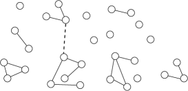
Figure 6: A random graph. The dashed line indicates a newly-added link that joins two randomly-selected nodes. The probability of joining together two components that contain $i$ and $j$ nodes is proportional to $ij$.

3.1 The Size Distribution

A random graph is grown from an initially disconnected graph with $N$ nodes. Two nodes are then selected at random and are connected. This process occurs at a constant rate, that we set equal to unity without loss of generality. This linking is repeated indefinitely until all $N$ nodes form a single connected component.

Let $n_{k}$ be the number of components of size $k$. The normalized density $c_{k}=n_{k}/N$ evolves according to the Smoluchowski equation

$$\frac{dc_{k}}{dt}=\frac{1}{2}\sum_{i+j=k}ijc_{i}c_{j}-k\,c_{k}.$$ (29)

The initial conditions are $c_{k}(0)=\delta_{k,1}$. In writing (29), the conservation law $\sum_{k}kc_{k}=1$ is employed. Equations (29) reflect that components are linked with a rate proportional to the product of their sizes.

The generating function $F(z,t)=\sum_{k}kc_{k}(t)e^{kz}$, evolves according to ${\partial F\over\partial t}=(F-1){\partial F\over\partial z}$ with the initial condition $F(z,0)=e^{z}$. Writing the derivatives through Jacobians, ${\partial F\over\partial t}={\partial(F,z)\over\partial(t,z)}$ and ${\partial F\over\partial z}={\partial(F,t)\over\partial(z,t)}$, and using the relation ${\partial z\over\partial t}={\partial(z,F)\over\partial(t,F)}$, the nonlinear equation for $F(z,t)$ is recast into the linear equation ${\partial z\over\partial t}=1-F$, from which we get $z(t)=(1-F)t+\ln F$. Exponentiating this equality gives an implicit relation for the generating functions

$$F(z,t)\,e^{-tF(z,t)}=e^{z-t}.$$ (30)

The Lagrange inversion formula conveniently yields the size distribution jbm ; hez

$$c_{k}(t)=\frac{(kt)^{k-1}}{k\cdot k!}e^{-kt}.$$ (31)

The system undergoes a gelation transition at time $t_{g}=1$. At this point a giant component arises that eventually engulfs the entire mass in the system. Close to the gelation time, the size distribution attains the scaling behavior

$$c_{k}(t)\simeq k_{*}^{-5/2}\Phi(k/k_{*}),$$ (32)

with the scaling function $\Phi(z)=\frac{1}{\sqrt{2\pi}}z^{-5/2}e^{-z/2}$. The typical size diverges, $k_{*}\simeq(1-t)^{-2}$, as $t\to t_{g}$. Beyond the gelation point, there exists an infinite sequence of transitions at times $t_{k}\simeq k^{-1}\ln N$ beyond which components of size $k$ disappear. At the last such transition time $t_{1}$, the system consists of the giant component and a few surviving monomers. The smallest component is always a monomer and the laggard problem is trivial.

3.2 The Leader

The size of the giant component (the last emerging leader) follows from the size distribution. Exactly at the gelation time, the large-size tail of the size distribution is algebraic, $c_{k}(t=1)\sim k^{-5/2}$, so that the cumulative distribution is $u_{k}\sim Nk^{-3/2}$. The criterion $u_{l_{w}}\sim 1$ gives the average size of the giant component $l_{w}\sim N^{2/3}$ bb and the time at which it emerges is $1-t_{w}\sim N^{-1/3}$.

Consider the size of the leader, $l(t,N)$, and the number of lead changes $L(t,N)$. At early times ($t\ll 1$), the behavior is the same as for random trees: the size of the leader $l(t,N)$, the number of lead changes $L(t,N)$, as well as the number of distinct leaders are all of the order $\ln N$. The asymptotic time regime in this case is $t\to 1$, as suggested by the size distribution. The tail of the size distribution together with $u_{l}=1$ yield an implicit relation for the size of the leader, $l\simeq 2(1-t)^{-2}\,\ln N-3(1-t)^{-2}\,\ln l\,$. Substituting the zeroth order approximation $l^{(0)}=2(1-t)^{-2}\,\ln N$ into $\ln l$ and ignoring subdominant $\ln\ln N$ terms gives the leader size

$$l(t,N)\simeq\frac{2}{(1-t)^{2}}\,\ln[N(1-t)^{3}].$$ (33)

At early stages ($t\ll 1$) the leader size grows logarithmically with the system size. Moreover, the leader size is proportional to the typical size but with a logarithmic enhancement.

The rate of leadership change is estimated as in the random tree case and we find $\frac{d}{dt}\,L(t,N)=(1-t)\,l(t,N)$, so that the time dependence of the number of lead changes is

$$L(t,N)\simeq 2\,\ln N\,\ln\frac{1}{1-t}-3\left[\ln\frac{1}{1-t}\right]^{2}\,.$$ (34)

It follows that the scaling form is

$$L(t,N)\simeq(\ln N)^{2}\,F(x)\qquad x=\frac{\ln\frac{1}{1-t}}{\ln N},$$ (35)

with the scaling function $F(x)=2x-3x^{2}$. This scaling function is related to the leader size: $l(t,N)\simeq k_{*}\ln Nf(x)$, with $f(x)=\frac{d}{dx}F(x)=2-6x$. The scaling behavior is obeyed until the giant component emerges, i.e., up to a time $t_{w}$, with $1-t_{w}\sim N^{-1/3}$. We neglected extremely slowly growing terms that are of the order $\ln\ln N/\ln N$ to obtain the scaling behavior. Thus, the approach to the scaling behavior may be very slow.

The total number of lead changes, $L(N)\simeq\frac{1}{3}(\ln N)^{2}$, is similar to the random tree case. Furthermore, the distribution of lead changes is Poissonian, as in (10), and the survival probability decays according to (12).

Random trees and random graphs show very different size characteristics. Gelation occurs in one case but not in the other. Nevertheless, leadership statistics in these two systems are remarkably similar. In both cases, the total number of lead changes grows as $L(N)\sim(\ln N)^{2}$. Moreover, the seemingly different scaling variables underlying (8) and (35) can be both related to the typical size $x=\ln k_{*}/\ln N$.

4 Random Networks

In the case of sequentially growing networks, the basic quantity is the degree distribution $N_{k}$, defined as the number of nodes of degree $k$ when the network contains $N$ total nodes. In this section, we investigate extremal properties of the degree distribution. We are again interested in the leader, namely, the node with the highest degree and its associated statistical properties.

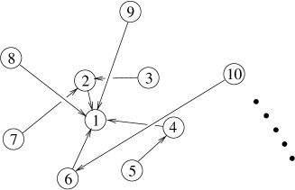
Figure 7: A random network. The network is grown by adding links sequentially. A new node has a single outgoing link that joins to an earlier node of degree $k$ with an attachment rate $A_{k}$. Each node is labeled by its index $J$.

4.1 Identity of the Leader

We characterize the $J^{\rm th}$ node that enters the network as having an index $J$ (Fig. 7). To start with an unambiguous leader node, we initialize the system to have $N=3$ nodes, with the initial leader having degree 2 (and index 1) and the other two nodes having degree 1. A new leader arises when its degree exceeds that of the current leader.

For a constant attachment rate ($A_{k}=1$), the average index of the leader grows algebraically, $J_{\rm lead}(N)\sim N^{\psi}$, with $\psi\approx 0.41$. The leader is typically an early node (since $\psi<1$), but not necessarily one of the very earliest. For example, a node with index greater than 100 has a probability of approximately $10^{-2}$ of being the leader in a graph of $N=10^{5}$ nodes. Thus the order of node creation plays a significant but not deterministic role in the identity of the leader node for constant attachment rate — there is partial egalitarianism.

We can understand this behavior analytically from the joint index-degree distribution. Let $C_{k}(J,N)$ be the average number of nodes of index $J$ and degree $k$. For constant attachment rate, this joint distribution obeys the rate equation

$${\partial C_{k}\over\partial N}={\partial C_{k}\over\partial J}+{C_{k-1}-C_{k}\over N}+\delta_{k1}\delta(N-J).$$ (36)

This is a slight generalization of the rate equation for the degree distribution itself KR01 . The new feature is the first term on the right that accounts for node “aging”.

The homogeneous form of this equation implies a self-similar solution. Thus, we seek a solution as a function of the single variable $J/N$ rather than two separate variables KR01

$$C_{k}(J,N)=f_{k}(x)\qquad{\rm with}\quad x=\frac{J}{N}.$$ (37)

This turns Eq. (36) into the ordinary differential equation

$$-x\,{df_{k}\over dx}=f_{k-1}-f_{k}.$$ (38)

We have omitted the delta function term, since it merely provides the boundary condition $c_{k}(J=N,N)=\delta_{k,1}$, or $f_{k}(1)=\delta_{k,1}$. The solution is simply the Poisson distribution in the variable $\ln x$, i.e.,

$$C_{k}(J,N)=\frac{J}{N}\,\frac{|\ln(J/N)|^{k-1}}{(k-1)!},$$ (39)

from which the average index of a node of degree $k$ is

$$J_{k}(N)=\frac{\sum_{1\leq J\leq N}J\,C_{k}(J,N)}{{\sum_{1\leq J\leq N}C_{k}(J,N)}}=N\left({2\over 3}\right)^{k}.$$ (40)

Thus the index of the leader is $J_{\rm lead}(N)=N(2/3)^{k_{\rm max}}$. The maximum degree is estimated from the extreme value criterion $\sum_{k\geq k_{\rm max}}N_{k}(N)\approx 1$ and using $N_{k}(N)=N/2^{k}$ KR01 gives $k_{\rm max}\sim{\ln N/\ln 2}$. Therefore kr

$$J_{\rm lead}(N)\sim N^{\psi},\qquad{\rm with}\qquad\psi=2-\frac{\ln 3}{\ln 2}\cong 0.415\,037,$$

in excellent agreement with numerical results.

For the linear attachment rate, $A_{k}=k$, numerical simulations indicate that a rich gets richer phenomenon arises, as the average index of the leader $J_{\rm lead}(N)$ saturates to a finite value of approximately 3.4 as $N\to\infty$. With probability $\approx 0.9$, the leader is among the 10 earliest nodes, while the probability $\approx 0.99$ the leader is among the 30 earliest nodes kr . In general, we find similar behavior for the more general case of the shifted linear attachment rate $A_{k}=k+\lambda$.

We can understand these results analytically through the joint index-degree distribution. For the linear attachment rate one has KR01

$$C_{k}(J,N)=\sqrt{J\over N}\left(1-\sqrt{J\over N}\right)^{k-1},$$ (41)

from which $J_{k}(N)=12N/[(k+3)(k+4)]$. Since $N_{k}(N)\simeq 4N/k^{3}$ for linear attachment BA ; KR01 , the extreme statistics criterion now gives $k_{\rm max}\sim N^{1/2}$. Therefore $J_{\rm lead}(N)\simeq 12N/k_{\rm max}^{2}={\cal O}(1)$ indeed saturates to a finite value. Thus the leader is one of the first few nodes in the network.

4.2 Number of Lead Changes

In contrast with random trees and random graphs, the average number of lead changes $L(N)$ grows only logarithmically in $N$ for both the attachment rates $A_{k}=1$ and $A_{k}=k$. While the average number of lead changes appears to be universal, there is a significant difference in the distribution of the number of lead changes, $P_{n}(N)$, at fixed $N$. For $A_{k}=1$, this distribution is sharply localized, while for $A_{k}=k$, $P_{n}(N)$ has a significant large-$n$ tail. This tail stems from repeated lead changes among the two leading nodes. Related to lead changes is the number of distinct nodes that enjoy the lead over the history of the network. Simulations indicate that this quantity also grows logarithmically in $N$.

This logarithmic behavior can be easily understood for the attachment rate $A_{k}=1$. Here the number of lead changes cannot exceed an upper bound given by the maximal degree $k_{\rm max}\sim\ln N/\ln 2$. To establish the logarithmic growth for the general attachment rate $A_{k}=k+\lambda$, we first note that when a new node is added, the lead changes if the leadership is currently shared between two (or more) nodes and the new node attaches to a co-leader. The number of co-leader nodes (with degree $k=k_{\rm max}$) is $N/k_{\rm max}^{3+\lambda}$, while the probability of attaching to a co-leader is $k_{\rm max}/N$. Thus the average number of lead changes satisfies

$${dL(N)\over dN}\sim{k_{\rm max}\over N}\,{N\over k_{\rm max}^{3+\lambda}}.$$ (42)

Since $k_{\rm max}\sim N^{1/(2+\lambda)}$, Eq. (42) reduces to ${dL/dN}\sim N^{-1}$ and thus gives the logarithmic growth $L(N)\sim\ln N$.

4.3 Fate of The First Leader

We now turn to the probability that the first leader retains the lead throughout the network growth. For the linear attachment rate $A_{k}=k+\lambda$ (rich get richer systems), the initial leader has a finite chance to remain in the lead forever. However, for the egalitarian attachment rate $A_{k}=1$, the initial leader is eventually replaced by another leader. Here, the probability that the initial leader retains the lead decays very slowly in time with an unusual decay law.

To understand the fate of the initial leader, we need to understand the degree distribution of the first node. We can straightforwardly determine this degree distribution analytically for the constant and linear attachment rates kr ; DMS2 . Let $P(k,N)$ be the probability that the first node has degree $k$ in a network of $N$ links. For $A_{k}=k$, this probability obeys kr

$$P(k,N+1)={k-1\over 2N}\,P(k-1,N)+{2N-k\over 2N}\,\,P(k,N).$$ (43)

The first term on the right accounts for the case that the earliest node has degree $k-1$. Then a new node attaches to it with probability $(k-1)/2N$, thereby increasing the probability for the node to have degree $k$. Conversely, with probability $(2N-k)/2N$ a new node does not attach to the earliest node, thereby giving the second contribution to $P(k,N+1)$.

The solution to Eq. (43) for the “dimer” initial condition $\circ\!$ $\!\circ$ is

$$P(k,N)={1\over 2^{2N-k-1}}\,{(2N-k-1)!\over(N-k)!\,(N-1)!}\,.$$ (44)

For $N\to\infty$, this simplifies to the Gaussian distribution

$$P(k,N)\simeq{1\over\sqrt{\pi N}}\,\,e^{-k^{2}/4N}$$ (45)

for finite values of the scaling variable $k/N^{1/2}$. Thus the typical degree of the first node is of the order of $N^{1/2}$; this is the same scaling behavior as the degree of the leader node. For the trimer initial condition (which we typically used in simulations) we obtain the degree distribution of the first node as a series of ratios of gamma functions in which $P(k,N)$ has an $e^{-k^{2}/4N}$ Gaussian tail, independent of the initial condition. The degree of the first node also approximates that of the leader node more and more closely as the degree of the first node in the initial state is increased MAA02 .

Although $P(k,N)$ contains all information about the degree of the first node, the behavior of its moments $\langle k^{a}\rangle_{N}=\sum k^{a}P(k,N)$ is simpler to appreciate. To determine these moments, it is more convenient to construct their governing recursion relations directly, rather than to calculate them from $P(k,N)$. Using Eq. (43), the average degree of the first node satisfies the recursion relation $\langle k\rangle_{N+1}=\langle k\rangle_{N}\left(1+{1\over 2N}\right)$ whose solution is

$$\langle k\rangle_{N}=\Lambda\,{\Gamma\left(N+\frac{1}{2}\right)\over{\Gamma\left(\frac{1}{2}\right)\Gamma(N)}}\simeq{\Lambda\over\sqrt{\pi}}\,N^{1/2}\,.$$ (46)

The prefactor $\Lambda$ depends on the initial conditions, with $\Lambda=2,8/3,16/5,\ldots$ for the dimer, trimer, tetramer, etc., initial conditions.

This multiplicative dependence on the initial conditions means that the first few growth steps substantially affect the average degree of the first node. For example, for the dimer initial condition, the average degree of the first node is, asymptotically, $\langle k\rangle_{N}\simeq 2\sqrt{N/\pi}$. However, if the second link attaches to the first node, an effective trimer initial condition arises and $\langle k\rangle_{N}\simeq(8/3)\sqrt{N/\pi}$. Thus, small initial perturbations lead to huge differences in the degree of the first node.

An intriguing manifestation of the rich get richer phenomenon is the behavior of the survival probability $S(N)$ that the first node leads throughout the growth up to size $N$ (Fig. 8). For the linear attachment rate, $S(N)$ saturates to a finite non-zero value of approximately 0.277 as $N\to\infty$; saturation also occurs for the general attachment rate $A_{k}=k+\lambda$. We conclude that for popularity-driven systems, the rich get richer holds in a strong form—the lead never changes with a positive probability.

Figure 8: The probability that the first node leads throughout the evolution obtained from $10^{5}$ realizations of up to size $N=10^{7}$ for $A_{k}=k$ (upper), and up to $N=10^{8}$ for $A_{k}=1$ (lower).

For constant attachment rate, $S(N)$ decays to zero as $N\to\infty$, but the asymptotic behavior is not apparent even when $N=10^{8}$. A power law $S(N)\sim N^{-\phi}$ is a reasonable fit, but the local exponent is still slowly decreasing at $N\approx 10^{8}$ where it has reached $\phi(N)\approx 0.18$. To understand the slow approach to asymptotic behavior, we study the degree distribution of the first node. This quantity satisfies the recursion relation

$$P(k,N)={1\over N}\,P(k-1,N-1)+{N-1\over N}\,P(k,N-1)$$ (47)

which reduces to the convection-diffusion equation

$$\left({\partial\over\partial\ln N}+{\partial\over\partial k}\right)P={1\over 2}\,{\partial^{2}P\over\partial k^{2}}$$ (48)

in the continuum limit. The solution is a Gaussian

$$P(k,N)\simeq{1\over\sqrt{2\pi\ln N}}\,\exp\left[-{(k-\ln N)^{2}\over 2\ln N}\right].$$ (49)

Therefore the degree of the first node grows as $\ln N$, with fluctuations of the order of $\sqrt{\ln N}$. On the other hand, the maximal degree grows faster, as $\ln N/\ln 2$, with negligible fluctuations.

We now estimate the large-$N$ behavior of $S(N)$ as $\sum_{k\geq k_{\rm max}}P(k,N)$. This approximation gives

$$S(N)\sim\int_{v\ln N}^{\infty}{dk\over\sqrt{\ln N}}\exp\left[-{(k-\ln N)^{2}\over 2\ln N}\right]\sim N^{-\phi}\,\,(\ln N)^{-1/2}\,,$$ (50)

with $\phi=[(\ln 2)^{-1}-1]^{2}/2\cong 0.097989$. The logarithmic factor leads to a very slow approach to asymptotic behavior.

The above estimate is based on a Gaussian approximate for $P(k,N)$ which is not accurate for $|k-\ln N|\gg\sqrt{\ln N}$. However, we can determine $P(k,N)$ exactly because its defining recursion formula, Eq. (47), is closely related to the Stirling numbers ${N\brack k}$ of the first kind stir . For the dimer initial condition, the solution reads $P(k,N)={N\brack k}/N!$. The corresponding generating function is stir

$$S_{N}(x)=\sum_{k=1}^{N}P(k,N)\,x^{k}={x(x+1)\ldots(x+N-1)\over N!}\,.$$ (51)

Using the Cauchy theorem, we express $P(k,N)$ in terms of the contour integral $S_{N}(x)/x^{k+1}$. When $N\to\infty$, this contour integral is easily computed using the saddle point technique. Finally, we arrive at Eq. (50) with the same logarithmic prefactor but with the slightly smaller exact transcendental exponent $\phi=1-\frac{1+\ln\ln 2}{\ln 2}\cong 0.08607$. The remarkably small exponent value and the logarithmic correction are the reasons why simulations with $N=10^{8}$ observed an exponent that was more that twice larger.

5 Summary and Discussion

Extremal properties provide an important statistical characterization of random structures and these properties yield many insights and surprises. Generally, extremes involve logarithmic dependences on system size. The practical consequences are numerous: slow convergence to asymptotic behavior, significant statistical fluctuations, erratic changes in extremal characteristics, and sensitive dependence on the initial conditions. Such behavior is consistent with our experience. For example, changes in athletic records are rare and unpredictable. As another example, the number of changes in the composition of the bellwether Dow Jones stock index (the 30 largest companies) ranged from a high of 11 in the 1990’s to a low of 0 in the 1950’s djia .

Leadership statistics of random graphs and random trees are quite similar: lead changes are infrequent; their total number increases logarithmically with the system size. The time-dependent number of lead changes approaches a self-similar form. The convergence to the asymptotic behavior is much slower for extremal statistics compared with size statistics because of the presence of various logarithmic dependences. Hence, the asymptotic behavior is difficult to detect in practice, especially for random graphs.

The most elementary leadership characteristic is the overall number of lead changes as a function of system size. This quantity can be measured simply by counting the number of changes until the process ends, making no reference to time. We have seen that introducing the time variable and treating the merger process dynamically not only produces this quantity, but also reveals an important self-similar behavior throughout the growth process.

Lead changes are also rare in popularity-driven network growth processes, where leadership is restricted to the earliest nodes. With finite probability, the first node remains the leader throughout the evolution. For growth with no popularity bias, leadership is shared among a somewhat larger cadre of nodes. As a consequence, the average index of the leader node grows algebraically with the network size. The possibility of sharing the lead among a larger subset of nodes gives a rich dynamics in which the probability that the first node retains the lead decays algebraically with the system size.

Extremal height properties of random trees can be obtained by analyzing the underlying nonlinear evolution equations. The cumulative distributions of tree heights approach a traveling wave form and the mean values grow logarithmically with the tree size. The corresponding growth coefficients can be obtained using either an elementary probabilistic argument or using an extremum selection criteria on the traveling wave. The same formalism used to analyze the leader and the laggard extends naturally to extremal statistics of extremal characteristics such as the heights of the tallest and the shortest trees.

To obtain leader or laggard characteristics, we employed the scaling behavior of the size distribution outside the scaling regime, namely, at sizes much larger than the typical size where, at least formally, statistical fluctuations can no longer be ignored. Nevertheless, the size dependences for these various leadership statistics appear to be asymptotically exact. Further analysis is needed to illuminate the role of statistical fluctuations, for example, by characterizing corrections to the leading behavior aal ; jls ; ve .

6 Acknowledgments

We are thankful to our collaborator Satya Majumdar. This research was supported by DOE(W-7405-ENG-36) and NSF(DMR0227670).

References

- (1) See, e. g., The Guiness Book of World Records (Downtown Book Center, Inc., 2001).
- (2) E. J. Gumbel, Statistics of Extremes (Columbia University Press, New York, 1958).
- (3) J. Galambos, The Asymptotic Theory of Extreme Order Statistics (R.E. Krieger Publishing Co., Malabar, 1987).
- (4) R. E. Ellis, Entropy, Large Deviations, and Statistical Mechanics (Springer-Verlag, New York, 1985).
- (5) D. Carpentier and P. Le Doussal, Phys. Rev. E 63, 026110 (2001)
- (6) D.S. Dean and S.N. Majumdar, Phys. Rev. E 64, 046121 (2001)
- (7) S. Raychaudhuri, M. Cranston, C. Pryzybla, and Y. Shapir, Phys. Rev. Lett. 87, 136101 (2001)
- (8) H. M. Mahmoud, Evolution of Random Search Trees (John Wiley & Sons, New York, 1992).
- (9) D. E. Knuth, The Art of Computer Programming, vol. 3, Sorting and Searching (Addison-Wesley, Reading, 1998).
- (10) W. Szpankowski, Average Case Analysis of Algorithms on Sequences (John Wiley & Sons, New York, 2001).
- (11) M. V. Smoluchowski, Z. Phys. Chem. 92, 215 (1917).
- (12) S. Chandrasekhar, Rev. Mod. Phys. 15, 1 (1943).
- (13) R. van Zon, H. van Beijeren, and Ch. Dellago, Phys. Rev. Lett. 80, 2035 (1998).
- (14) B. Bollobás, Random Graphs (Academic Press, London, 1985).
- (15) S. Janson, T. Łuczak, and A. Rucinski, Random Graphs (John Wiley & Sons, New York, 2000).
- (16) P. J. Flory, Principles of Polymer Chemistry (Cornell, Ithaca, 1953).
- (17) G. U. Yule, Phil. Trans. Roy. Soc. B 213, 21 (1924); The Statistical Study of Literary Vocabulary (Cambridge University Press, Cambridge, 1944).
- (18) H. A. Simon, Biometrica 42, 425 (1955); Infor. Control 3, 80 (1960).
- (19) W. Willinger, R. Govindan, S. Jamin, V. Paxson, and S. Shenker, Proc. Natl. Acad. Sci. 99, 2573 (2002).
- (20) See e.g., S. H. Strogatz, Nature 410, 268 (2001).
- (21) B. Skyrms and R. Pemantle, Proc. Natl. Acad. Sci. 97, 9340 (2000).
- (22) M. Girvan and M. E. J. Newman, Proc. Natl. Acad. Sci. 99, 7821 (2002).
- (23) O. C. Martin, R. Monasson, and R. Zecchina, Theor. Comput. Sci. 265, 3 (2001).
- (24) H. Nishimori, Statistical Physics of Spin Glasses and Information Processing (Oxford University Press, New York, 2001).
- (25) M. Mezard, G. Parisi, and G. Zecchina, Science 297, 812 (2002).
- (26) J. Baik, math-PR/0310347
- (27) P. L. Ferrari, M. Prähofer, H. Spohn, math-ph/0310053.
- (28) C. Knessl and W. Szpankowsky, SIAM J. Comput. 30, 923 (2000).
- (29) See e.g., the annual list of the 400 wealthiest individuals in Fortune Magazine.
- (30) T. Hattori and H. Ochiai, preprint (1998).
- (31) P. L. Krapivsky and S. N. Majumdar, Phys. Rev. Lett. 85, 5492 (2000).
- (32) B. Pittel, J. Math. Anal. Appl. 103, 461 (1984).
- (33) L. Devroye, J. ACM 33, 489 (1986).
- (34) P. Noguiera, Disc. Appl. Math. 109, 253 (2001).
- (35) S. N. Majumdar and P. L. Krapivsky, Phys. Rev. E 65, 036127 (2001).
- (36) For a recent review, see D. Aldous, Bernoulli 5, 3 (1999).
- (37) E. Ben-Naim and P. L. Krapivsky, Europhys. Lett., in press.
- (38) E. Ben-Naim, P. L. Krapivsky, and S. N. Majumdar, Phys. Rev. E 64, 035101(R) (2001).
- (39) J. D. Murray, Mathematical Biology (Springer-Verlag, New York, 1989).
- (40) M. Bramson, Convergence of Solutions of the Kolmogorov Equation to Travelling Waves (American Mathematical Society, Providence, R. I., 1983).
- (41) W. van Saarloos, Phys. Rev. A 39, 6367 (1989).
- (42) E. Brunet and B. Derrida, Phys. Rev. E 56, 2597 (1997).
- (43) U. Ebert and W. van Saarloos, Phys. Rev. Lett. 80, 1650 (1998); Physica D 146, 1 (2000).
- (44) S. N. Majumdar and P. L. Krapivsky, Physica A 318, 161 (2003).
- (45) D. Stauffer, Introduction to Percolation Theory, (Taylor & Francis, London, 1985).
- (46) H. S. Wilf, Generatingfunctionology (Academic Press, Boston, 1990).
- (47) J. B. McLeod, Quart. J. Math. Oxford 13, 119 (1962); ibid 13, 193 (1962); ibid 13, 283 (1962).
- (48) E. M. Hendriks, M. H. Ernst, and R. M. Ziff, J. Stat. Phys. 31, 519 (1983).
- (49) P. L. Krapivsky and S. Redner, Phys. Rev. E 63, 066123 (2001).
- (50) P. L. Krapivsky and S. Redner, Phys. Rev. Lett. 89, 258703 (2002).
- (51) A.-L. Barabási and R. Albert, Science 286, 509 (1999).
- (52) S. N. Dorogovtsev, J. F. F. Mendes, and A. N. Samukhin, Phys. Rev. E 63, 062101 (2001).
- (53) A. A. Moreira, J. S. de Andrade Jr., and L. A. N. Amaral, Phys. Rev. Lett. 89, 268703 (2002).
- (54) J. Stirling, Methodus Differentialis (London, 1730); see also R. L. Graham, D. E. Knuth, and O. Patashnik, Concrete Mathematics: A Foundation for Computer Science (Reading, Mass.: Addison-Wesley, 1989).
- (55) http://indexes.dowjones.com.
- (56) A. A. Lushnikov, J. Colloid Inter. Sci. 65, 276 (1977).
- (57) J. L. Spouge, J. Colloid Inter. Sci. 107, 38 (1985).
- (58) P. G. J van Dongen and M. H. Ernst, J. Stat. Phys. 49, 879 (1987).