A spectroscopic cell for fast pressure jumps across the glass transition line

Abstract

We present a new experimental protocol for the spectroscopic study of the dynamics of glasses in the aging regime induced by sudden pressure jumps (crunches) across the glass transition line. The sample, initially in the liquid state, is suddenly brought in the glassy state, and therefore out of equilibrium, in a four-window optical crunch cell which is able to perform pressure jumps of 3 kbar in a time interval of $\approx$10 ms. The main advantages of this setup with respect to previous pressure-jump systems is that the pressure jump is induced through a pressure transmitting fluid mechanically coupled to the sample stage through a deformable membrane, thus avoiding any flow of the sample itself in the pressure network and allowing to deal with highly viscous materials. The dynamics of the sample during the aging regime is investigated by Brillouin Light Scattering (BLS). For this purpose the crunch cell is used in conjunction with a high resolution double monochromator equipped with a CCD detector. This system is able to record a full spectrum of a typical glass forming material in a single 1 s shot. As an example we present the study of the evolution toward equilibrium of the infinite frequency longitudinal elastic modulus ($M_{\infty}$) of low molecular weight polymer (Poly(bisphenol A-co-epichlorohydrin), glycidyl end capped). The observed time evolution of $M_{\infty}$, well represented by a single stretched exponential, is interpreted within the framework of the Tool-Narayanaswamy theory.

I introduction

Glass forming materials can relax their structure on a timescale which is dramatically sensitive to control parameters (temperature, pressure, etc.) in the vicinity of the glass transition region. When approaching the glass phase boundary, the typical structural relaxation time increases by several orders of magnitudes until the system falls out of equilibrium on a macroscopic timescale. The physical properties of the so formed glasses depend on history and evolve with the time spent in the glassy phase. Microscopic dynamics progressively slows down and the system is said to display physical aging. The possibility of recovering a thermodynamic description of glasses in terms of additional, slowly time dependent, state parameters is still a lively debated issue in condensed matter physics davies ; McKenna ; cugliandolo97 ; nieu ; SciortinoTh ; dileo . In this respect, the development of any new experimental protocol capable to probe the aging dynamics of glass-forming materials, is crucial to verify and stimulate existing theories of the glassy state. Out of equilibrium states are customarily produced by fast cooling (quench). In this case the cooling time depends on both the quenching rate and the time required for the sample temperature to equilibrate at the thermostat temperature. This latter contribution can be estimated considering that the thermal diffusivity of a non metallic liquid is of order $D_{T}\sim 10^{-7}m^{2}/s$ and that the typical linear sample dimension in a light scattering experiment (the one presented here) is $L\sim 1$ cm:

$$\tau_{eq}\simeq\frac{1}{D_{T}q^{2}}\simeq 1\;\textrm{min}$$

Even in the (non physical) case of infinite quenching rate, the above observation implies that one is practically obliged to quench the sample to temperatures below the glass transition temperature $T_{g}$ (where the structural relaxation time $\tau_{\alpha}$ reaches $100$ s) and to perform experiments lasting for hours or even days macphail .

The rapid production of non-equilibrium states in glass forming systems opens, therefore, new possibilities for the spectroscopic investigation of the aging regime: i) there is no need to perform long experiments, the dynamics can be sampled on the time-scale of seconds, ii) the aging dynamics for sufficiently long times does not depend on the detailed thermodynamic history. The investigation of the aging regime over reasonably short time-scales can be in principle achieved through an alternative choice of the control parameter, namely performing rapid pressure jumps (crunches). In fact, pressure propagates inside the sample with the speed of sound, that means:

$$\tau_{eq}\simeq\frac{L}{c}\simeq 10\;\mu\textrm{s}$$

In this conditions what really fixes the crunch time is the minimum time required to stabilize the pressure on the walls of the sample cell to the new value, i.e. the experimental crunching rate.

Pressure jumps have been often used in the past, particularly to perform studies on chemical reactions kinetic and on protein unfolding. To our knowledge no attempt has been made to use the crunches to attain out-of-equilibrium states in disordered matter. The pressure ”jump” (or pressure perturbation as usually called in the chemical kinetic studies) are used to control the reactions equilibrium constant via the modulation of the system free energy, ruled in turn by the pressure. The response of the system is then detected through the time dependence of the systems conductivity or optical properties. This method, tracing back to the works of Maxfield et al.CleggMaxfield , is capable of fast (20 $\mu$s) but moderate (few bar) pressure variation (for a recent review see WuLin ). In this type of experiments the cell is usually a two-windows optical cell, with sapphire windows and the pressure modulation is attained through a stack of piezoelectric crystals. When larger pressure variation is needed, the procedure consists in slowly increasing the pressure of the liquid sample up to the burst of a safety membrane, which causes the sudden pressure release. Up to 200 bar in $\approx$100 $\mu$s has been reached with this method Astumian .

An ”optical” two-windows cell, suitable for light- and neutron-scattering experiments has been recently employed to study phase transitions. In this case Migler large pressure ”jump” are needed. This is accomplished by controlling the pressure of a transmitting fluid (silicon oil) separated from the sample by a deforming gasket (viton o-ring). In this case, however, due to the mechanical pressure control, the pressure variation were limited to 30 bar/s. Therefore only ”slow” pressure changes were allowed by this setup.

More recently, an high pressure jump apparatus devoted to X-ray studies of protein folding has been recently proposed by Woenckhaus et al. woe . This setup is capable of liquid-liquid pressure jumps with a maximum amplitude of $7$ kbar on a time scale of $5$ ms. Such a jump is achieved by loading the sample at high pressure in a storing chamber separated from the measurement chamber (two-windows sample cell) by a high pressure valve, then quickly opening the valve. While this scheme can be profiting exploited in the study of liquid-to-liquid pressure jump, it presents conceptual shortcomings if one aims to perform jumps ending up in the glass phase or in a supercooled liquid phase. Indeed, in the latter cases, the sample in the storage chamber is already highly viscous, consequently the time needed to flow throughout valves and pipes is long enough to slow-down the pressure change. To overcome this problem a pressure transmitting fluid -physically separated from the sample- is mandatory.

The drawback of having the sample in the whole high pressure network has been overcome by a novel design set-up StKr . This set-up mixes the fast negative pressure jump obtained by Woenckhaus et al. woe (i.e. it makes use a fast high pressure valve) with the idea of having a transmitting fluid separated by the sample (in this case by a teflon piston). The sample cell is a two-windows X-ray cell suitable for small-angle x-ray scattering, and extensively used to follow the time evolution of biological samples. The maximum pressure jump is $-3.5$ kbar and the typical time needed for such jump is $5$ ms, i.e. the time needed to open the high pressure valve.

In this paper we describe the layout of a new set-up that is designed to match the following requests: i) four-windows optical cell to perform light-scattering experiment (two-windows cell are not suitable as the back-scattering geometry must be avoided due to the intrinsic high level of stray light not compatible with a CCD based detection system, see below); ii) possibility to perform liquid-to-glass and glass-to-glass transition, i.e. the sample need to be separated by the pressure transmitting fluid; iii) initial and final pressure controlled in the widest possible range ($P_{i},\;P_{f}<7$ Kbar, $\Delta P<2$ Kbar); iv) quick positive pressure change ($\approx 5$ ms); v) possibility of automatic and quick repetition of the ”crunches”. This framework is based on a pressure transmitting fluid that couples a sealed but deforming sample stage to an expansion gas chamber. In the following we present the details of the device, along with an example of its application. In particular we study aging effects on the sound velocity (determined from the dynamic structure factor measured by Brillouin Light Scattering) of a glass forming material, Poly(bisphenol A-co-epichlorohydrin), glycidyl end capped (PBGD), after a pressure jump from the liquid to the glassy phase close to the glass transition pressure.

II The crunch cell

Figure 1: Schematic layout of crunch apparatus. After the evacuation of the low- and high-P chambers, the gas reservoir is used to fill the low pressure chamber to the desired pressure and the pressure generator (a manual Nova Swiss piston) brings the sample to the initial pressure.

The layout of our apparatus consists of two main stages (Fig. 1). A low pressure chamber is loaded with gas (Nitrogen) through a feed line designed to operate at a maximum pressure of 700 bar (typical working values are 50 bar).

Figure 2: Details of the high pressure chamber. The piston is mechanically connected to a piston in the low-P chamber (are ratio 1:50) and has a maximum excursion of 10 mm.

A piston mechanically couples the low pressure stage to a chamber filled with ethanol (the pressure transmitting medium). This high pressure stage (Fig. 2) mainly consists of a tempered steel cell. Four quartz optical windows in right angle geometry allows for either 90 degrees, forward or back-scattering geometries. One feed-through allows the pressure transmitting fluid loading through an high pressure line connected to a pressure generator Nova Swiss (7 kbar max). Two further feeds connect an high pressure gauge and a thermocouple. All the connectors, valves and tubes where purchased from Nova Swiss, Switzerland.

The two surfaces of the piston are such that the equilibrium position is reached when the pressure of the fluid in the sample cell is $\sim$ 50 times bigger than that of the gas. The crunch event is obtained by the following steps:

1. an electro-magnet is switched on blocking the piston in its upper position (smallest volume in the gas chamber, biggest in the transmitting fluid chamber),

2. the pressure of the transmitting fluid is brought to the desired initial value ($1\div 700\textrm{bar}$) by means of an hand-screw-type pressure generator,

3. the gas chamber is filled up to $\sim 60\textrm{bar}$ according to the final value desired for the pressure in the sample cell (max $3000\textrm{bar}$),

4. the electromagnet is switched off releasing the piston which compresses the transmitting fluid to the final pressure.

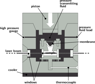
Figure 3: Expansion of the lower part of the four optical windows high pressure chamber with the sample container (four optical windows and an elastic membrane to equalize the pressure on the pressure transmitting fluid and on the sample.

A small brass cell (Fig. 3) with a flexible membrane and four optical quartz windows is filled with sample and immersed in the pressure transmitting fluid. The membrane mechanically couples the sample to the pressure transmitting fluid. The pressure of the sample is monitored indirectly by means of an high pressure strain gauge in contact with the fluid. The temperature is read on a thermocouple fixed on the stem of the sample cell.

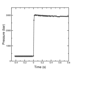
Figure 4: Time dependence of the pressure during a crunch event in a test experiment on iso-pentane. The pressure has been measured by a pressure (strain) gauge coupled to the transmitting fluid at a sampling rate of 100 Hz.

In standard operation, all the pressure and the temperature gauges are monitored by means of Gefran 2300 fast display units connected to the serial port of a PC. The maximum recording rate for pressure is $100\textrm{Hz}$. In the commissioning phase, the pressure gauge is read via a digital oscilloscope in order to trace the pressure change in the sample with the desired time resolution. A typical pressure profile of a test fluid (iso-pentane) in the sample chamber during a crunch event is reported in Fig. 4. As can be noticed, in this example the pressure jumps from $\sim 300\textrm{bar}$ up to $\sim 3000$ in $\sim$ 10 ms and the temperature changes by $\approx$2 K (strongly sample dependent). The subsequent slow ($\sim$ 0.5 s) decrease of pressure is due to the thermalization of the fluids to room temperature. The low compressibility of the gas (as compared to those of the pressure transmitting fluid and of the sample) guarantees the pressure stability against small volume rearrangement due to the (expected) slow time dependence of the compressibility in the aging sample. The latter point is important as, with respect to other set-ups , the present device is designed to work at constant pressure, even in presence of relaxation in the physical properties of the sample.

III An application: aging of the dynamic structure factor

III.1 Experimental details and results

As an example of application of the crunch apparatus we present the investigation of aging effects in the dynamics of Poly(bisphenol A-co-epichlorohydrin), glycidyl end capped (PBGD). In particular we monitor the time evolution of the infinite frequency longitudinal elastic modulus $M_{\infty}$ (defined as the instantaneous part of pressure response to an infinitesimal relative volume variation) as determined from the dynamic structure factor obtained by Brillouin Light Scattering (BLS). We will discuss the results in the framework of the old fictive pressure concept firstly introduced by Tool and co-workers TN . The Brillouin light scattering spectra are measured by a CCD- and monochromator-based system. The incoming beam, $500$ mW at $\lambda$=514.5 nm , from a Coherent INNOVA Ar-ion laser operating in single mode owing to an intra-cavity ethalon and in power-stabilized mode, was focused on the sample. The polarization of the incident beam is vertical with respect to the scattering plane. The light, scattered at an average angle of $90$, was collected by a field lens ($20$ cm focal length, 4 cm diameter). After selecting the vertical polarization by a polaroid film (rejection $10^{-4}$), the scattered light is focused on the entrance slit (20 $\mu$m in the dispersion plane $\times$ 2 mm) of a SOPRA DMDP2000 monochromator. The latter is composed of a couple of two meter focal length grating monochromators, in Fastie-Ebert mounting, each one with entrance and exit slits and coupled in additive dispersion by an external 1:1 telescope. The monochromator was operating in the single pass/double monochromator (DMSP) configuration sopra at the 11-th diffraction order, corresponding to a transmissions of $\approx 25\%$ and a total dispersing power on the exit slit plane equal to 1 cm^-1/mm. In a conventional experiment all the slits are closed according to the desired resolution width, a photo-multiplier is placed in front of the exit slit and frequency scans of scattered light are obtained by simultaneous rotation of the two gratings. In this operating mode a full Brillouin spectrum with good statistic is acquired in $30-60$ minutes. For the reasons discussed in the introduction one aims to reduce the observation time as much as possible, to tens of ms having in mind that the crunch event lasts for $\approx 10$ ms. In this respect the use of a CCD detector turns out to be an appropriate choice as it allows the detection of a full Brillouin spectrum, with a good statistics, in less than one second. Therefore, in our setup, the two intermediate slits and the exit slit of the monochromator are fully open (2 mm $\times$ 2 mm) and the image formed in the final plane slit is focused via of a single achromat doublet (focal length 75 mm, magnification $\sim 10$) on the surface of a CCD camera. The choice of the focusing lens has been done in order to maintain aberrations well below the monochromator’s resolution. The camera is a HiResIII camera (DTA, Pisa, Italy) mounting a SITe 1100x330 pixel (total dimension 2 mm $\times$ 0.6 mm) back-illuminated CCD sensor (quantum efficiency of $\sim 80\%$) cooled via a Peltier element and a fluid close circuit system based on an HAAKE 75 refrigerator. In this set up, the spectral range covered by the CCD sensor is 2 cm^-1, i.e. 0.002 cm^-1/pixel, that correspond to ten points on each spectral resolution as dictated by the width of the monochromator entrance slit. The image of the camera is transferred to a PC, where the BLS spectrum is obtained by integrating the image in vertical (non-dispersing) dimension, and by performing the usual operation (background subtraction, flat field correction, etc.)

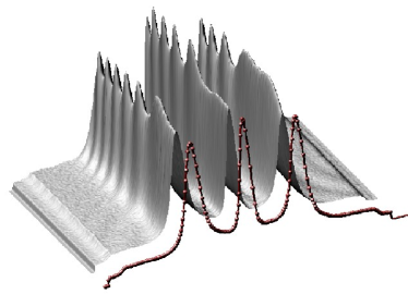
Figure 5: Three-dimensional image of the intensity measured by the CCD detector (exposure time $10s$) on a sample of toluene. The surface represents the light intensity while the line is the average intensity over CCD rows orthogonal to the dispersion direction of the spectrometer. The intensity oscillation are due to interference in the CCD silicon wafer. The intensity drops in the far tails of the Brillouin triplet is due to the spectral cut of the 1 mm width intermediate slits of the spectrometer.

As an example, in Fig. 5 we show the Brillouin spectrum of Toluene in a $90^{\circ}$ scattering geometry at ambient temperature and pressure. The exposure time is only 10 s, but the statistical quality of data is comparable to that of a 1000 s long frequency scan performed with photo-multiplier. In the 3-D plot a fringes pattern due to interference of coherent light reflected by the (non-wedged) CCD array surface is clearly visible. The presence of such a fringe pattern is not relevant in the present application as the final information is obtained integrating the image in the vertical dimension (full line in the figure) and, therefore, the intensity oscillation introduced by the interference is averaged out. The spectra is made by the well-know triplet of lines. The central one brings contribution from the entropic mode (thermal diffusion process) and from the structural relaxation (Mountain peak, non visible here as the toluene at room condition has a relaxation time much shorter than the inverse of the frequencies covered in Fig. 5. The side peaks are due to the pressure modes, and, in particular, their frequency position and width bring information on the elastic moduli and on the liquid viscosity. Equilibrium spectra like that in Fig. 5 are used to calibrate the frequency scale on the CCD surface, i.e. the pixel-to-wavenumber conversion factor.

A second calibration, which will turn out useful in the data analysis, is the relation existing, for the specific investigated sample, between the applied pressure and the elastic modulus for the liquid at equilibrium.

Figure 6: Example of Brillouin spectra of (equilibrated) PBGD at room pressure (open circles) and at 2 Kbar (full circles) in the crunch cell. The intense elastic line is due to both parasitic light coming from the optical windows and from the mountain mode (which become quasi-elastic in the investigated thermodynamic conditions) of PBGD.

In Fig. 6 we report as an example the spectrum of PBGD at room temperature and $P$=1, 2000 bar. As in the case of toluene, the spectra shows the three peaks structure of Brillouin spectra of liquids. In this case the central component is the sum of three unresolved contributes i) the Rayleigh line: light scattered by the slow decaying component of density fluctuation driven by thermal diffusion ($\tau\sim 1\mu s$); ii) the Mountain line: light scattered by the slow decaying component of density fluctuation driven by structural relaxation ($\tau>1\mu s$); iii) the Stray light: light scattered elastically by particles in the sample and optical components (windows, lenses, etc.). In addition to the central component the spectra display also a clearly visible Brillouin doublet arising from acoustic damped oscillations in the density fluctuation decay. Since the frequency of these oscillations is of order $10$ GHz all the previously mentioned slow modes are basically frozen on the acoustic timescale the peak position ($\omega_{\infty}$) is obtained from the infinite frequency modulus:

$$\omega_{\infty}^{2}=\frac{q^{2}n^{2}}{\rho}M_{\infty}.$$

$$M_{\infty}=V\left(\frac{\partial P}{\partial V}\right)_{S,\xi}$$

Where the subscripts $S$ and $\xi$ mean that the thermodynamic derivative has to be computed for constant entropy (frozen thermal diffusion) and fixed structure (frozen structural relaxation). Since the variation of $n^{2}/\rho$ with pressure turns out to be much more weak than that of $M_{\infty}$, $\omega_{\infty}^{2}$ is basically proportional to $M_{\infty}$.

We have fitted the Brillouin peaks with two Lorentzians in order to get information on the peak position and indirectly on $M_{\infty}$. These equilibrium spectra have been measured from $P$=0 to $P$=2.9 kbar, each time waiting for the system to equilibrate before performing the data collection. It is worth noticing that in this pressure range the relaxation time of PBGD (as determined by dielectric/PCS spectroscopy, paluchprl ) are in the 0.1$\div$100 ms range.

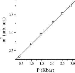
Figure 7: Squared frequency of Brillouin peaks ($\circ$) as function of pressure for equilibrated PBGD. The solid line represents the best fit with a linear law

The calibration measurement, reported in Fig. 7, indicates that $\omega_{\infty}^{2}(P)$ is linearly proportional to the pressure in the investigated pressure range. This result, as we will see later, simplifies the data analysis however is not crucial. Indeed, even in the case of non-linear relation between moduli and pressure, the calibration curve can be used to extract the time evolution of the (apparent) pressure from that of the moduli.

As an example of crunch experiment, in Fig. 8 we report a (selection of) CCD images with exposure time $1$ s following a pressure jump from $0.6$ to $2.6$ kbar. Each image displays the three peaks structure of Brillouin spectra of liquids. We have fitted the Brillouin peaks with two Lorentzian lines in order to get information on the peak position and indirectly on $M_{\infty}$. The obtained values, reported as a function of time in Fig. 9, are very well represented by a stretched exponential law. In the following section we will show that such a stretched exponential behavior is consistent with the prediction of the Tool-Narayanaswamy model in the approximation of a very fast crunch.

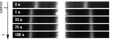
Figure 8: CCD images of Brillouin spectra of PBGD at different waiting times during the aging dynamics. The intense central peak and the two weaker side peaks are clearly visible. Time zero indicate the spectra taken just before the crunch. Soon after the crunch the Brillouin peaks jumps to a new value, which then slowly changes during the aging process.

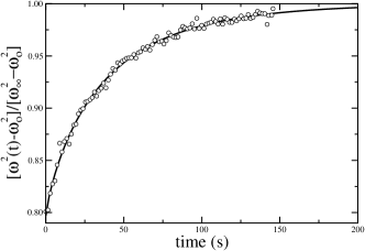
Figure 9: Plot of the infinite frequency modulus (open circles) as a function of waiting time $t_{w}$ after the crunch. The initial 80% of the change in $\omega^{2}$ is due to the ”vibrational” component rearrangement, the residual 20% -shown here- is the slow structural rearrangement. The solid line is a fit to the expected stretched exponential behavior with $\tau,\beta$ free parameters.

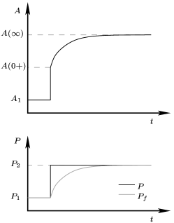
Figure 10: The upper panel reports a sketch of the expected time evolution of a generic macroscopic observable $A$ after a crunch from $P_{1}$ to $P_{2}$. The time dependence of the external (thick line) and fictive (thin line) pressures are qualitatively reported in the lower panel.

III.2 The Tool-Narayanaswamy model

Consider a supercooled liquid, initially at equilibrium, whose pressure is abruptly changed from $P_{1}$ to $P_{2}$. The time evolution of a generic macroscopic observable $A$ is sketched in Fig. 10. As rapidly as the pressure is changed $A$ jumps from $A_{1}$ (equilibrium value at $P=P_{1}$) to $A(0+)$ in a glass-like fashion, i. e. similarly to what would have been happened if the $P_{1}\rightarrow P_{2}$ jump was taking place in the deep glassy state, when only the vibrational degrees of freedom are free to rearrange and the structure is frozen. This initial, adiabatic, modification of $A$ is followed by a slow structural relaxation, during which the observable $A$ changes with time from $A(0+)$ to the new equilibrium value $A(\infty)$. Let’s call $\phi$ the relaxational part of $A(t)$:

$$\phi(t)=\frac{A(\infty)-A(t)}{A(\infty)-A(0+)}$$

The ”fictive pressure” is a variable introduced for computational and conceptual convenience and represents $\phi$ in units of pressure:

$$P_{f}=P_{2}-(P_{2}-P_{1})\phi(t)$$ (1)

The relevance of the concept of ”fictive pressure” lies in the observation that, while we know that at equilibrium $A$ is a well defined function of pressure and temperature, we argue that out of equilibrium the state of the system is specified only if we know the additional state variable $P_{f}$. This quantity evolves from $P_{1}$ to $P_{2}$, reflecting the slow evolution of the system’s structure towards equilibrium.

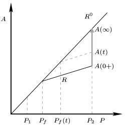
Figure 11: Expected pressure dependence of a generic observable $A$.

In those cases where $A$ depends linearly on pressure $P_{f}$ assumes a more physical interpretation. Let’s consider an equilibrated liquid system at initial pressure $P_{1}$, compressed with a finite compression rate $R=dP/dt$. Initially, the equilibrium relaxation time is so short that the system will adiabatically follow the pressure change, and the variable $A$ evolves along its equilibrium curve (from $P_{1}$ to $P_{f}$ in Fig. 11). At a given pressure ($P_{f}$) the relaxation time becomes so long that the system falls out of equilibrium, and the variable $A$ follows a weaker (solid-like, here assumed linear and not depending on $R$) $P$ dependence (from $P_{f}$ to $P_{2}$). The so defined $P_{f}$ is a function of the compression rate $R$ and in particular will be greater the slower is $R$. The value $A(0+)$ reached after the compression will also depend on $R$ or, equivalently, on $P_{f}$: $A(0+)=A(T,P_{2},P_{f})$. Inverting the last equality we obtain $P_{f}=P_{f}(T,P_{2},A)$. Once the final pressure is reached, and $A$ is equal to $A(0+)$, the aging process starts. $A$ evolves toward $A(\infty)$ and to each $A(t)$ we can associate a fictive pressure $P_{f}(t)$ following the dashed line in Fig. 11 which is the one defined in (1). If the so defined fictive pressure is a true state variable the value of $P_{f}$ obtained from (1) has the special meaning of that pressure where the system would fall out of equilibrium in a compression experiment leading directly to $A(t)$.

The structural relaxation process in the aging regime is both non-exponential and non linear. The most widely applied treatment of this features is embodied in what is called the Tool-Narayanaswamy (TN) model TN , which postulates the following expression for $\phi(t)$:

$$\phi(t)=\sum_{i}g_{i}\exp\left[-\int_{0}^{t}\frac{dt^{\prime}}{\tau_{i}(P,P_{f})}\right]$$ (2)

The non-exponential character of the relaxation is accounted for by invoking a distribution of relaxation times $\tau_{i}$ with weights $g_{i}$. The non-linear character is accounted for by allowing the relaxation times to depend both on pressure, $P$, and on the average structural state of the system as measured, for example, by $P_{f}$. The number of adjustable parameters entering in this model can be considerably reduced if one assumes a continuous spectrum of relaxation times, which shape is specified by a single, pressure independent parameter and its location on a logarithmic timescale is specified by a reference relaxation time $\tau$ ($\tau_{i}=\tau/\lambda_{i}$). The most common choice for the spectrum of relaxation times is the Kohlrausch-Williams-Watts (KWW) or stretched exponential function:

$$\sum_{i}g_{i}\exp\left(-\frac{t}{\tau_{i}}\right)=\sum_{i}g_{i}\exp\left(-\lambda_{i}\frac{t}{\tau}\right)=\exp\left[-\left(\frac{t}{\tau}\right)^{\beta}\right]$$ (3)

On a general ground, the relaxation in response to a complicated pressure history, e.g., a pressure jump $\Delta P_{1}$ at time $t_{1}$, $\Delta P_{2}$ at $t_{2}$, …$\Delta P_{m}$ at $t_{m}$, may be dealt with by invoking the superposition principle TN , so that the fictive pressure $P_{f}(t)$ at time $t>t_{m}$ is given by:

$$P_{f}(t)=P_{1}+\sum_{j=0}^{m}\Delta P_{j}[1-\phi(t-t_{j})]$$ (4)

or in integral form:

$$P_{f}(t)=P_{1}+\int_{0}^{t}R(t^{\prime})\left[1-\phi(t-t^{\prime})\right]dt^{\prime}$$ (5)

where $R=dP/dt$ is the compression rate. In order to solve (5) we need an explicit form for $\tau(P,P_{f})$. The simplest choice comes from the observation that for short enough pressure intervals $\tau(P)$ for an isothermal equilibrated sample is well described by:

$$\tau_{eq}(P)=\tau_{0}\exp(\alpha P)$$ (6)

The simplest generalization is that of replacing $P$ in (6) with a linear combination of $P$ and $P_{f}$ montrose :

$$\tau=\tau_{0}\exp\left[\alpha(xP+(1-x)P_{f})\right]$$ (7)

which reduces to (6) in the equilibrium case ($P_{f}=P$).

III.3 Evolution of fictive pressure in the crunch approximation

If we crunch a system from $P_{1}$ to $P_{2}$ the subsequent evolution of fictive pressure will depend on the pressure profile as expressed by (5). In these circumstances (5) has to be integrated numerically bezot . However if the compression is fast enough $R(t)$ in (5) can be replaced by $(P_{2}-P_{1})\delta(t)$ and the detailed shape of the pressure profile during the compression becomes irrelevant:

$$P_{f}(t)=P_{2}-\Delta\phi(t),\;\;\;\Delta=P_{2}-P_{1}$$ (8)

Substituting (2) and(3) in (8) we obtain:

$$\phi(t)=\frac{P_{2}-P_{f}(t)}{\Delta}=\exp\left[-\left(\int_{0}^{t}\frac{dt^{\prime}}{\tau(P_{2},P_{f}(t^{\prime}))}\right)^{\beta}\right]$$ (9)

and by inserting (7):

$$\phi(t) = \exp\left[-\left(\frac{\xi(t)}{\tau_{eq}(P_{2})}\right)^{\beta}\right]$$ (10)

$$\xi(t) = \int_{0}^{t}\exp\left[\bar{\alpha}\phi(t^{\prime})\right]dt^{\prime}$$ (11)

where the dimensionless parameter $\bar{\alpha}$ is equal to $\alpha(1-x)\Delta$. Equation (11) cannot be solved analytically but we provide here an approximated solution which holds in an easy estimable range of times. We start by assuming that $\phi(t)$ is well represented by the stretched exponential:

$$\phi(t)\simeq\exp\left[-\left(\frac{t}{\tau^{*}}\right)^{\beta^{*}}\right]$$ (12)

In the logarithmic time interval $|\ln(t)-\ln(\tau^{*})|\ll 1/\beta^{*}$ one can replace the stretched exponential in (12) with:

$$\exp\left[-\left(\frac{t}{\tau^{*}}\right)^{\beta^{*}}\right]\simeq\frac{1}{e}\left(\frac{t}{\tau^{*}}\right)^{-\beta^{*}}$$ (13)

which substituted in (11) and using (13) once again gives:

$$\xi(t)=at^{b},\;\;\;b=1-\frac{\bar{\alpha}\beta^{*}}{e},\;\;\;a=\frac{(e{\tau^{*}}^{\beta^{*}})^{\frac{\bar{\alpha}}{e}}}{b}$$ (14)

Substituting the above expression for $\xi(t)$ in (11) and equating the result to (12) we obtain $\tau^{*}$ and $\beta^{*}$ as functions of $\tau_{eq}(P_{2})$, $\beta$ and $\bar{\alpha}$:

$$\tau^{*}=\tau_{eq}(P_{2})\frac{e^{-\frac{\bar{\alpha}}{e}}}{1+\frac{\bar{\alpha}\beta}{e}}\;\;,\;\;\;\;\beta^{*}=\frac{\beta}{{1+\frac{\bar{\alpha}\beta}{e}}}$$ (15)

This result is based on the approximation (13) which holds in a wider time range the smaller is $\beta^{*}$. Since $\beta^{*}$ decreases with increasing $\bar{\alpha}=\alpha(1-x)\Delta$ we can conclude that for big pressure jumps ($\Delta$) we expect, on the basis of TN model, that the aging dynamics of a generic observable, linearly dependent on $P_{f}$, could be described by stretched exponential with parameters $\tau^{*},\beta^{*}$ in Eq. (15).

A fit (Fig. 9) to the experimental data with a stretched exponential function with $\tau,\beta$ as free parameters shows indeed a very good qualitative agreement with the TN model predictions. It is not our aim here to discuss the physical meaning of these parameters, we want only to stress the importance of making experiments with a high compression rate that lead to easy-to-interpret results (see Eq. LABEL:taubetai).

IV Conclusions

We presented an experimental device able to perform crunch events, specifically fast pressure jumps of the order of 3 Kbar, in a time interval shorter than 10 ms. The sample is confined in a small environment which is mechanically coupled to the pressure transmitting fluid by a flexible membrane. Such a configuration allows the possibility of performing fast crunches into highly viscous phases opening the way to investigations of aging dynamics on the timescale of seconds. An experimental setup, based on the crunch cell and on a double grating monochromator equipped with a CCD detector, has been developed and used to collect Brillouin spectra with a repetition rate of $\sim 1$ s during an aging regime with characteristic timescale of $\approx 100s$. The aging of the dynamic structure factor of s typical polymeric glass former has been studied and, in particular, the relaxation of the infinite frequency longitudinal modulus has been reported as a function of waiting time. A stretched exponential behavior has been found and justified according to the Tool-Naranayaswamy fictive pressure model. The systematic study of nonlinear modulus relaxation for pressure jumps of increasing entity will be performed in order to verify or discard the prediction obtained in Sec. III.3.

References

- (1) R.O. Davies, G.O. Jones, Adv. Phys. 2, 370 (1953).
- (2) G. B. McKenna in Comprehensive Polymer Science, Vol. 2, Polymer Properties, ed. by C. Booth and C. Price, Pergamon, Oxford (1989), p 311.
- (3) L.F. Cugliandolo, J. Kurchan, L. Peliti, Phys. Rev. E 55, 3898 (1997).
- (4) Th.M. Nieuwenhuizen, Phys. Rev. Lett. 80, 5580 (1998).
- (5) S. Mossa, E. La Nave, F. Sciortino, and P. Tartaglia Eur. Phys. J. B 30, 351 (2002).
- (6) R. Di Leonardo, A Taschin, R. Torre, M. Sampoli, and G. Ruocco, Physical Review E 67, 015102 (2003).
- (7) R. S. Miller and R. A. MacPhail, J. Chem. Phys., 106, 3393, (1997).
- (8) R. M. Clegg and B. W. Maxfield, Rev. Sci. Instrum., 47, 1383, (1976).
- (9) C.-H. Wu, C.-F. Lin, S.-L. Lo and T. Yasunaga, Proc. Natl. Sci. Counc., ROC(A), 23, 466, (1999).
- (10) R. D. Astumian, M. Sasaki, T. Yasunaga and Z. A. Schelly, J. Phys. Chem., 85, 3832, (1981).
- (11) K. B. Migler and C. C. Han, Macromolecules, 31, 360, (1998).
- (12) J. Woeckhaus, R. Köhling, R. Winter, P. Thiyagarajan, and S. Finet, Rev. Sci. Instr. 71 3895 (2000).
- (13) M. Steinhart, M. Kriechbaum, K. Pressl, H. Amenitsch, P. Laggner, and S. Bernstorff, Rev. Sci. Instrum., 70, 1540, (1999).
- (14) O.S. Narayanaswamy, J. Am. Ceram. Soc.54, 491, (1971)
- (15) P. Benassi, V. Mazzacurati, G. Ruocco, Eng. Optics 11, 533 (1988); ibid. J. of Phys. E 21, 798 (1988).
- (16) M. Paluch, A. Patkowski, and E.W. Fischer, Phys. Rev. Lett, 85, 2140, (2000).
- (17) D.M. Heyes and C.J. Montrose, Trans. ASME F 105, 280, (1980)
- (18) P. Bezot and C. Hesse-Bezot, J. Non-Cryst. Solids 122, 160 (1990).